


Abstract
Membrane waves propagating along the cell circumference in a top down view have been observed with several eukaryotic cells (Döbereiner et al 2006 Phys. Rev. Lett. 97 10; Machacek and Danuser 2006 Biophys. J. 90 1439–52). We present a mathematical model reproducing these traveling membrane undulations during lamellipodial motility of cells on flat substrates. The model describes the interplay of pushing forces exerted by actin polymerization on the membrane, pulling forces of attached actin filaments on the cell edge, contractile forces powered by molecular motors across the actin gel and resisting membrane tension. The actin filament network in the bulk of lamellipodia obeys gel flow equations. We investigated in particular the dependence of wave properties on gel parameters and found that inhibition of myosin motors abolishes waves in some cells but not in others in agreement with experimental observations. The model provides a unifying mechanism explaining the dynamics of actin-based motility in a variety of systems.
Export citation and abstract BibTeX RIS

Content from this work may be used under the terms of the Creative Commons Attribution-NonCommercial-ShareAlike 3.0 licence. Any further distribution of this work must maintain attribution to the author(s) and the title of the work, journal citation and DOI.
1. Introduction
Experiments have shown traveling membrane protrusions or retractions in many cell types such as mouse embryonic fibroblasts, fly wing disc cells, mouse T cells and Dictyostelium discoideum [1, 3, 6–8]. These waves can be identified as the dynamics of the cell contour in a top down view of the cell on the substrate. The contour dynamics consists sometimes of homogeneous oscillations rather than propagating structures [8]. Membrane waves are believed to play a central role in cell motility, endocytosis and probing the extracellular matrix [9]. In the damped liquid environment of the cell, these propagating waves are maintained by active forces from the cytoskeleton. Actin polymerization produces most of the driving force for membrane protrusion [10]. Polymerization also creates a network of actin filaments providing support for the forces acting on the membrane. The network of actin filaments is cross-linked by various proteins. Among them, myosin II molecular motors not only cross-link but can also contract the network. Some of the membrane waves disappear upon inhibition of contraction of the actin gel [1, 3, 4, 7, 11], and others exist without myosin activity [1–6, 8]. This suggests that the membrane waves are driven by the protrusive force of actin polymerization and the contractile stress produced by myosin II molecular motors contributes in some cases only.
Several theoretical approaches have been introduced to explain the mechanism responsible for membrane wave propagation. In the approach of [12–14], membrane waves are driven by curvature-mediated activation of actin polymerization. A non-decaying membrane wave was produced by the coupling between membrane shape and protrusive–contractive forces of actin–myosin and the addition of only convex actin activators in this model [13]. The intrinsic curvature values that can be induced or are preferred by membrane proteins suggest that the mechanism applies to ruffle-like waves [14]. The observation of a transition between homogeneous oscillations with vanishing curvature and waves of the cell contour induced by signaling mechanisms suggests that different dynamic regimes of one system defined by different parameter values produce both the phenomena. The homogeneous oscillations are unlikely to be produced by a mechanism relying on curvature.
Here we propose a mechanism for membrane wave generation that does not require any spontaneous curvature of actin polymerization activators. The dynamics of the cell boundary, and therefore cell shape, are determined by the interaction of actin filaments with cell membrane, cross-linking of actin filaments, polymerization- and myosin-driven retrograde flow of the actin gel and load due to membrane tension. In our model, while transiently membrane-bound filaments are pulling back the membrane, the polymerizing actin network pushes on the cell membrane from within (see figure 1). Membrane tension equilibrates spatially very fast, but temporarily varies with the cell's projected area. This introduces a global spatiotemporal coupling in the dynamics of distant regions on the cell boundary.
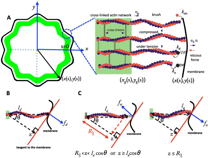
Figure 1. Schematic illustration of the interaction between the membrane and the actin cortex in a cell. (A) The actin network consists of two parts: a highly cross-linked actin meshwork (actin gel) and free actin filaments (semiflexible region (SR)). The membrane and the gel boundary are characterized in Cartesian coordinates by (x(s),y(s)) and (xg(s),yg(s)), respectively, with s being the contour length of the membrane or actin gel boundary. In the SR, filaments undergo cycles of attachment (ka) and detachment (kd): while detached filaments with contour length ld polymerize and push against the membrane (fd), attached filaments with contour length la can either pull or push the membrane (fa). Both pushing and pulling forces depend on the contour length of the filaments as well as the orientation of the filaments (θ) and the normal distance to the membrane (z). R∥ ≈ la[1 − la/4ℓp] cos θ is the projected equilibrium end-to-end distance of the polymer onto the membrane normal.
Download figure:
Standard image2. The model
The model is schematically represented in figure 1. The cell is characterized in Cartesian coordinates by x(s) and y(s) with s measuring the cell's contour length. The membrane at each small interval (s,s + ds) is pushed or pulled by actin filaments which are anchored in a highly cross-linked actin gel with a linear density nl. The gel forms due to cross-linking of actin filaments. The newly polymerized filaments are not yet cross-linked and therefore behave like an ensemble of individual filaments. We call the filamentous range a semiflexible region (SR) since its properties are dominated by the semiflexible filament behavior. It takes some time till that critical degree of cross-linking is reached, which turns the network into a gel. Newly polymerized filament parts move backwards during that time owing to retrograde flow. That turns the temporal transient into a spatial gradient of the degree of cross-linking. We define the location of the critical concentration of bound cross-linkers as the gel boundary. The gel boundary advances with a rate set by cross-linking and effectively shortens the free length of filaments in the SR. Since polymerization occurs at the leading edge membrane only, we obtain the lamellipodium structure shown in figure 1 with an SR at the leading edge and a gel further in the bulk. The complete protrusion is often described as consisting of the posterior lamellum with highly cross-linked and bundled actin filaments and the anterior lamellipodium, which is much less bundled. We do not identify the gel with the lamellum and the SR with the lamellipodium. However, we assume the gel boundary to be in the lamellipodium.
Cross-linkers dissociate from filaments deep in the bulk of the gel and diffuse back to the lamellipodium leading edge, where they can bind again. Solving the equations for this reaction–diffusion process explains the dependence of the gel boundary velocity on system parameters and variables [24]. The velocity increases with the free length of actin filaments with a characteristic length scale  and saturates at the maximum value vmaxg, which depends on the concentration of available cross-linkers [24]:

The SR at each interval (s,s + ds) is formed by populations of attached and detached filaments with linear densities na(s) and nd(s) and average contour lengths la and ld, respectively. Filaments bind transiently via linker proteins to the membrane. The filament's attachment rate to the linker protein on the membrane is ka. The filament–linker complex exerts force fa normal to the membrane during attachment. The linker proteins are modeled as springs with spring constant kl and zero equilibrium length. The force fa depends on kl, the filament's contour length la as well as on the distance between gel and membrane z. The filament–linker complex has a nonlinear force–extension relation which we approximate by a piece-wise linear function [20]. Let R∥ ≈ la[1 − la/4ℓp] cos θ be the projected equilibrium end-to-end distance of the polymer onto the membrane normal. The elastic response of filaments experiencing small compressional forces (z ⩽ R∥) is approximated by a spring constant k∥ = 12kBTℓ2p/l4a [21]. For small pulling forces (z ⩾ R∥), the linker–filament complex acts as a spring with an effective constant keff = klk∥/(kl + k∥). In the strong force regime, the force–extension relation of the filament is highly nonlinear and diverges close to full stretching [22]. Therefore, only the linker will stretch out. The complete force–extension relation is captured by
Attached filaments are usually under tension and detach with a force-dependent rate kd [23]

Here, k0d is the spontaneous detachment rate and δ ∼ 2.7 nm is one-half of the actin monomer size.
The pushing force due to actin polymerization near the edge is the main type of active force at the membrane. Detached filaments polymerize at subsecond timescales and exert normal protrusive force fd on the membrane. The membrane hinders the polymerization. The higher the filament pushing against the membrane is, the lower the polymerization velocity is. According to [43], vp decreases exponentially with fd:

with vmaxp = konδG the saturation polymerization velocity in the absence of any obstacle. kon is the monomer assembly rate and G is the actin monomer concentration. The pushing force fd of semiflexible polymers in the presence of an obstacle has been extensively studied in [19]. For a stiff polymer such as actin with persistence length ℓp = 15 μm and contour length ld ≪ ℓp, the pushing force can be approximated by  , in which fc = kBTℓp/l2d is the Euler buckling force and the scaling parameter ζ is given by ζ = ℓp(ld − z)/l2d. For a small compression (ζ ⩽ 0.2), the dimensionless force
  reads
reads
We now write the set of equations for the dynamics of the coupled system consisting of attached and detached filaments in the SR, the boundary of the cross-linked actin gel and the membrane [16]. The average lengths of attached and detached filaments in the interval (s,s + ds) are denoted by la and ld, respectively. The filament lengths shrink with velocity vg and grow only in the detached state by polymerization with velocity vp. The time evolution of the average number of attached filaments na is described by a constant attachment rate ka and a stress-dependent detachment rate kd. The gel boundary characterized by (xg,yg) advances with velocity vg and moves backward due to retrograde flow vr. Furthermore, the membrane resists motion with a drag force (coefficient η), and resists bending deformations defined by the local membrane curvature κ(s) due to membrane tension S. All these dynamic processes are captured by the following set of equations:


![$\bar v_{\mathrm {g}}=v_{\mathrm {g}}\,{\mbox {max}}[1,l/\sqrt {(x-x_{\mathrm {g}})^2+(y-y_{\mathrm {g}})^2}]$](https://content.cld.iop.org/journals/1367-2630/14/11/115002/revision1/nj436301ieqn4.gif) defines the local velocity of gelation and points in the direction normal to the gel boundary.
defines the local velocity of gelation and points in the direction normal to the gel boundary.Membrane tension imposes an opposing force on growing actin filaments at the cell's leading edge. Tension gradients in the membrane at any point equilibrate within milliseconds in a fluid membrane such as lipid membranes. Hence, on the scale of seconds and minutes relevant to cell motility, tension is constant along the cell boundary but can change with time [27, 28]. We hypothesize that membrane tension changes linearly with the cell's projected area:

in which S0 and S1 are constants and A0 is the cell's preferred area and deviations from this area produce an effective extra membrane tension. This implies a spatial long-range coupling of distant points on the membrane and may lead to different morphodynamic patterns on the membrane. We choose A0 = 60 μm2, which gives a cell radius of the order of 4.4 μm. This is the typical size of a D. discoideum cell. In addition, κ(s) is the signed local membrane curvature defined as

where ' and '' are the first and the second derivatives with respect to s.
In most motile cells, the actin network is simultaneously transported away from the leading edge in a process known as retrograde flow [34]. The flow is driven by the net force exerted by the SR on the leading edge membrane and contractile forces of myosin motors (μ). Friction of the flowing actin gel against the intracellular interface of cell adhesion complexes (ξ) and gel viscosity ηg damp retrograde flow. A semi-analytical solution of the corresponding gel equations in the radial direction provides the expression for retrograde flow vr as [24]

with a0ret and b0ret written as


We use this expression of retrograde flow calculated in a one-dimensional geometry as an approximation for the radial flow in our model cell in order to simplify the model. Exact calculation of retrograde flow would, of course, require the simulation of the two-dimensional gel equations [29, 31].
3. Results
3.1. Lateral traveling waves
We integrate numerically the set of differential equations (6) and combine time behavior with a stability analysis. The cell has a preferred radius R close to but larger than  . The cell shape is a circle initially. The distribution of actin filaments (n0l) and saturation polymerization speed (vmaxp) over the cell boundary is assumed to be uniform. Linear stability analysis illustrates that within certain ranges of polymerization, attachment, detachment and cross-linking, the starting fixed point is unstable. We choose that unstable state as the initial condition for the simulation. The cell contour reaches its asymptotic behavior after some transient (see, e.g., figure 3). The parameters μ and ξ are among important parameters governing the dynamic modes of the model described by equation (6) as can be seen in figure 2 (see [15, 16, 24] for bifurcation diagrams in dependence on SR parameters). The parameter μ corresponds to myosin activity and the friction coefficient ξ is proportional to the cell–substrate adhesion site density.
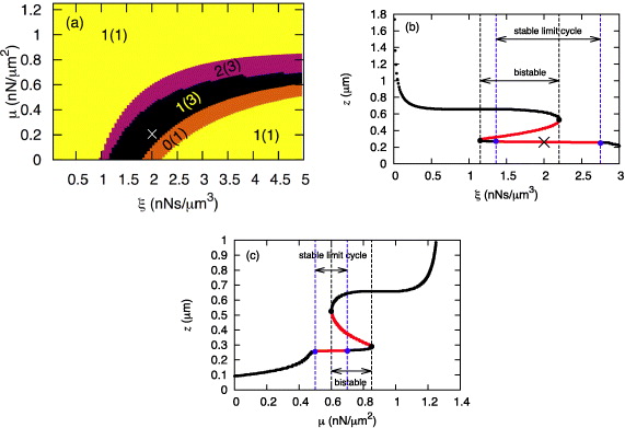
Figure 2. (a) Bifurcation diagram of the system described by equations (6) in the parametric plane μ–ξ. Displayed are the number of stable steady states and the total number of steady states (in parentheses). (b) Fixed points and linear stability for μ = 0.2 nN μm−2. Black (red) lines correspond to stable (unstable) states, respectively. The points mark saddle–node bifurcations (black) and Hopf bifurcations (blue). z is defined in figure 1. ' × ' in both figures denotes the parameter values for which the simulations in figure 3 were performed. (c) Fixed points and linear stability for ξ = 4.8 nN s μm−3. For the other parameters of the model, see table 1.
Download figure:
Standard imageTable 1. Table of parameters.
| Parameter | Symbol | Value | Remark |
|---|---|---|---|
| Actin monomer radius | δ | 2.7 nm | [35] |
| Persistence length of the actin filament | lp | 15 μm | [36] |
| Attachment rate | ka | 0.5 s−1 | Assumed |
| Detachment constant | k0d | 1 s−1 | 0.5 s−1 in [38] |
| Saturation value of cross-linking velocity | vmaxg | 30 nm s−1 | Assumed |
| Saturation length of cross-linking velocity |
 |
100 nm | Assumed |
| Saturation value of polymerization velocity | vmaxp | 140 nm s−1 | [30, 42] |
| Total filament density | n0l | 0.2 nm−1 | [32, 33] |
| Spring constant of the linker | kl | 0.7 pN nm−1 | [38, 39] |
| Effective drag coefficient | η | 4 pN s μm−2 | [40, 41] |
| Membrane tension | S0 | 10 pN | Assumed |
| Membrane tension coefficient | S1 | 10−2 pN nm−2 | Assumed |
| Active contractile stress in the actin gel | μ | 8.33 pN μm−2 | [25] |
| Friction coefficient modeling adhesion | ξ | 0.2–30 nN s μm−3 | [44, 45] |
| Height of the lamellipodium at the leading edge | h0 | 0.1 μm | [42, 46, 47] |
| Length of the gel part of the lamellipodium | L | 10 μm | [47, 48] |
| Viscosity of the actin gel | ηg | 270 nN s μm−2 | [44] |
In the regime with only unstable fixed points and a stable limit cycle, the membrane position oscillates, spatially desynchronizes and the cell exhibits lateral wave patterns propagating on the circumference. Since distribution of actin filaments is homogeneous on the cell edge, there is no net cell locomotion. The cell is spread on the substrate, has a roughly circular shape and the membrane periodically undergoes global shape changes.
Examples of the membrane normal velocity map and curvature map are shown in figures 3(a) and (b). The wave pattern is also visible in the other dynamic variables, such as polymerization velocity vp, radius of cell and gel boundaries, net normal velocity of the gel boundary, average length of attached and detached filaments (la,ld) and total pulling/pushing forces of bound/unbound filaments (nafa,ndfd) (see figures 3(c)–(j)). The cell and gel boundaries are measured with respect to the fixed origin at (0,0) (the laboratory frame of reference). Interestingly, the wave propagation is also observed in the net velocity of the gel boundary vg − vr as well as in the radius of the gel boundary (figures 3(c) and (j)). In this example, lateral speeds of membrane waves are of the order of 82 μm min−1 and the amplitude of the wave is about 100 nm. In order to understand the mechanism of wave propagation in figure 3, the time evolution of propulsive and retractive forces and velocities at a single point on the membrane (s = 0) are presented in figures 4(a) and (b).
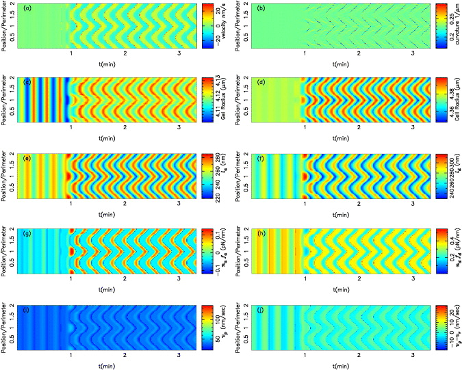
Figure 3. Color maps of the normal membrane velocity (a), curvature (b), gel boundary (c), cell boundary (d), averaged length of attached and detached filaments (e, f), total pulling and pushing forces per unit length (g, h), polymerization velocity (i) and net velocity of the gel boundary (j) along the contour over time of a cell exhibiting lateral membrane waves. Note the clear bands of protrusions (positive velocity or curvature) and retractions (negative velocity or curvature). The time between successive protrusions or retractions is T = 12.64 ± 0.48 s and the wavelength λ = 21.78 ± 7.093 μm is of the order of the cell's total contour length. Here vmaxg = 30 nm s−1, μ = 0.2 nN μm−2, ξ = 2 nN s μm−3 and all the other parameters are listed in table 1. The dimensionless position along the membrane is defined as s/l (l is the cell circumference), and all the color maps are plotted over two contour lengths to avoid loss of details.
Download figure:
Standard image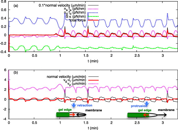
Figure 4. (a) The protrusion events (positive velocity) of the cell boundary at s = 0 are caused by a strong propulsive force of unbound actin filaments; however, membrane retractions (negative velocity) are due to (together) dominant pulling force of bound filaments and resisting membrane tension. (b) The membrane's retraction and protrusion velocities are almost of the same order of magnitude as the gel edge velocity, although out of phase: as the membrane retracts (v < 0), the gel boundary advances forward (vg − vr > 0) and vice versa. The transition from retractive to a protrusive state is the consequence of a significant increase in propulsive force (ndfd) and is associated with a sudden drop in polymerization velocity vp. All the parameters are the same as in figure 3.
Download figure:
Standard imageThe leading edge membrane velocity and gel boundary velocity are in antiphase during the oscillations shown in figure 4. When the membrane is pushed forward, the opposite force acts on the gel boundary, drives retrograde flow and tips the balance between flow and cross-linking to net inward. When the membrane is pulled inward, the opposite force slows down retrograde flow and the gel boundary moves outward. Oscillations and the alternating forces arise from an interplay of free filament length dynamics and attachment and detachment of filaments. The free filament length shortens during membrane retraction, since the gel boundary advances and the membrane retracts. Filaments become stiffer due to this shortening, which increases the force exerted by polymerizing filaments on the leading edge membrane. Attached filaments can stand that force for a while, but when it reaches a critical strength, they are ripped off the membrane. With little left holding it back, the membrane jerks forward and the phase of membrane protrusion starts. The total force on the membrane is pushing, now. The filament lengths grow and forces decrease, since longer filaments are less stiff. Therefore also the detachment rate decreases and filaments re-attach. That increases the pulling forces, which after some time cause the transition back to the retraction phase. Not all of the inward forces acting on the leading edge membrane are exerted by attached filaments. Membrane tension contributes a substantial part. However, the switches in the balance between pushing and pulling forces arise from the interaction between filament attachment and length dynamics.
Our model provides a unifying oscillation mechanism across different systems. The mechanism has been most clearly shown experimentally with oil drops by Trichet et al [50]. Trichet et al describe filament detachment and re-attachment as the processes in the core of the oscillation mechanism as in our model. A decrease of filament attachment by vasodilator-stimulated phosphoprotein (VASP) can lead to an onset of oscillatory motion both in experiments and in the model [50]. The amount of pushing and pulling forces acting on the oil drop is indicated by its degree of deformation from the spherical force free shape toward a kiwi shape [50]. The total force is proportional to the velocity. That allows us to directly read the phase relation between forces and velocity from movies of oil shape and motion such as supplementary movie 2 of [50]. Oil drops show increasing deformation in the slow velocity phase [50], indicating the rise of both ndfd and nafa. The release of these forces indicated by relaxation to a spherical shape coincides with an increase in velocity. Later, onset of deformation coincides with a decrease in velocity. This phase relation between forces and velocity agrees with our model results. The results of modeling the velocity time course of drop motion are presented in [17]. We show the phase relation between forces and velocities for drops in figure 5. As in the experiments, both ndfd and nafa increase during the slow velocity phase, a fast increase of the velocity coincides with a drop in the amount of forces and filament detachment. The high-velocity phase is terminated by re-attachment of filaments and an increase in both ndfd and nafa. The same phase relation applies to the oscillation mechanism of the cell simulations reported here. Merely, all velocity values are shifted toward negative velocities due to gel contraction and retrograde flow, and the values of nafa are smaller than ndfd due to membrane tension.
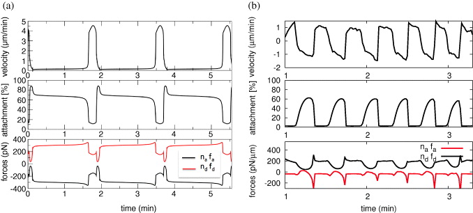
Figure 5. (a) Simulation of the oscillatory motion of oil drops. The pushing force ndfd rises slowly in the slow velocity phase. The pulling force nafa balances it up to the point when the attached filaments cannot stand it anymore. They detach avalanche-like and the oil drop jerks forward. The same phase relation applies to oscillations of the cell membrane velocity (b). See the text for details.
Download figure:
Standard imageAn example of wave propagation with faster protrusion–retraction events as well as larger wave amplitude is shown in figure 6. In this example, we determined the wave period T = 21.79 ± 4.09 at a given point i on the cell membrane as the maximum of the Fourier spectrum and subsequent averaging over all points. Similarly, we determined the spatial wavelength as time average λ = 10.42 ± 6.62 μm. In contrast to previous patterns, the wavelength is here much shorter than the cell circumference (about 1/3).

Figure 6. (a) The membrane's normal velocity and wave amplitude grow as the filament linear density n0l increases to 0.5 nm−1 and the surrounding fluid viscosity η decreases to 0.4 pN s μm−2. The other parameters are the same as in table 1 except that ka = 0.2 s−1, kd = 0.1 s−1, a0ret = 40 nm s−1 and b0ret = 80 nm pN−1 s−1 and vmaxg = 50 nm s−1. The cell contour (black line) and gel boundary (red line) motion are also illustrated by the supplementary movie 1 (available from stacks.iop.org/NJP/14/115002/mmedia).
Download figure:
Standard imageWe see in figure 6 more clearly than before that protrusions and retraction events are organized in lateral waves along the cell membrane. Notably, the bands of positive (protrusion) or negative velocity (retraction) make an angle with respect to the temporal axis. This indicates that protrusion or retraction are not happening simultaneously, but rather local protrusion or retraction activity propagates with a definite speed in either direction across the cell boundary. Lateral waves propagating in opposite directions collide and annihilate each other. Interestingly, membrane waves exist even in the absence of molecular motor contractile forces (μ = 0), as can be seen in figure 2.
We also looked at the dependence of wave period on myosin activity μ and adhesion strength ξ. Although the dependence of wavelength on ξ as well as μ was not significant (data not shown), reducing myosin contractile stress μ within the oscillatory regime increases the wave period significantly (figures 7(a) and (b)).

Figure 7. (a) Wave period T is plotted against the myosin activity parameter μ as the cell–substrate adhesion strength ξ is kept constant at 4.8 nN s μm−3 (lower red line in figure 2(c)). A small change in myosin activity has a significant effect on the wave period. (b) The wave period shows a biphasic behavior when the cell–substrate adhesion strength ξ is increased and the myosin activity parameter μ is kept constant at 0.2 nN μm−2 (lower red line in figure 2(b)).
Download figure:
Standard imageThe shape of protrusion or retraction events is sensitive to the attachment/detachment rates of the filaments to the membrane. Increasing ka generates more regular wave patterns on the membrane and increases the wavelength as well (see figure 8). The retraction velocity of the membrane is faster at high values of ka due to the higher number of attached filaments. On the other hand, fast membrane retraction buckles and shortens the unbound actin filaments generating a strong propulsive force which quickly dominates the resisting membrane tension and force of attached filaments and ultimately the membrane expands again (see figure 8(b)). The type and amplitude of wave pattern depend also on the cell size and the saturation length of the cross-linking velocity. In biological terms, that saturation length can be increased by decreasing the cross-linker binding rate [24]. Increasing the cell size weakens global coupling since relative area changes by protrusions are smaller. Simulations in figure 9 were carried out with a cell with a ten times larger preferred area A0 = 600 μm2 (the typical size of a fish keratocyte),  increased to 400 nm and all the other parameters are the same as in figure 6. The resulting wave pattern is completely different and the wave amplitude is larger (∼ 1 μm).
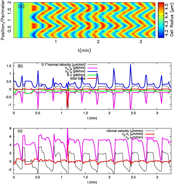
Figure 8. (a) Wave pattern is sensitive to the attachment rate of filaments ka. Increasing ka leads to a more regular wave pattern and increases the wavelength. (b) Time evolution of membrane velocity and forces acting on the membrane at the point s = 0. Here the wave period is T = 19.13 ± 2.09 s and the wavelength is λ = 20.99 ± 7.6 μm. All the parameters are the same as in figure 6 except for ka, which has increased to 0.5 s−1.
Download figure:
Standard image
Figure 9. A cell with larger preferred area A0 = 600 μm2 and larger  (saturation length of cross-linking velocity) has a completely different wave pattern and a larger wave amplitude (∼ 1 μm). For other parameters see figure 6. The cell contour (black line) and gel boundary (red line) motion are also illustrated by the supplementary movie 2 (available from stacks.iop.org/NJP/14/115002/mmedia).
Download figure:
Standard imageBecause membrane tension is constant along the cell boundary, it effectively couples protrusion and retraction events that take place in spatially distinct regions of the cell. Thus, membrane tension provides for a global coupling in membrane dynamics. Figure 10 shows a pattern typical of systems with global coupling [49]. It exhibits two different regions oscillating in synchrony (phase clusters) but with a phase difference between the regions. Due to an analogy to phase clusters in systems of discrete coupled oscillators, these patterns are called cluster patterns [49].

Figure 10. The circumference of a cell with a larger preferred area A0 = 600 μm2 is long enough for establishing another pattern type. It consists of two large synchronized regions oscillating with a constant phase difference. The pattern is typical of systems with global coupling provided here by the membrane tension. For the other parameter values see figure 3.
Download figure:
Standard imageExperiments on fibroblast and keratocyte cells show that cells spreading on a highly adhesive substrate exhibit traveling waves around the edge [26, 31], but a lack of cell–substrate adhesion can lead to a 'frustrated' instability in which wave propagation is blocked along the membrane but the cell edge oscillates [26]. Within our model parameters, in the limit of weak cell–substrate adhesion strength (ξ → 0), the retrograde flow coefficient b0ret increases significantly although a0ret approaches the constant value μL/8η (see equation (10)). To determine the effect of adhesion strength, we fixed the parameters as in figure 6, and selected b0ret to be a large value such as 800 nm pN−1 s−1, which corresponds to weak adhesion. In addition, we also decreased S1 to the value S1 = 10−5 pN nm−2, which allows larger variations in the cell's area. We observed that, in agreement with experiment, the formation of protrusion and retraction events is stopped and all the points along the membrane show synchronized oscillations (see figure 11).
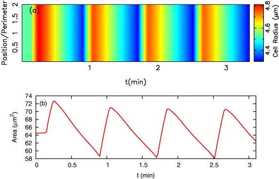
Figure 11. The adhesiveness of the substrate has an impact on the membrane instability. When there is a lack of cell–substrate adhesion (small ξ or large b0ret), traveling waves along the cell boundary disappear, but the cell radius and area show regular oscillations. Parameters are the same as in figure 6 except for b0ret = 800 nm pN−1 s−1 and S1 = 10−5 pN nm−2.
Download figure:
Standard image4. Discussion
The protrusions of cells spreading and resting or motile with well-developed lamellipodia consist of the posterior lamellum with highly cross-linked and bundled actin filaments and the anterior lamellipodium with a network of individual filaments polymerizing against the leading edge membrane. The circumference of the protrusions exhibits a variety of wave patterns. Alternating retractions and protrusions comprise in some cases the whole depth of the lamellipodium (see [1, 3] and possibly also [7]) and have in other cases an amplitude smaller than this depth [6–8]. The large-amplitude oscillations may involve cyclic (partial) loss of the lamellipodium and regeneration by nucleation of filaments and are therefore not covered by this study. They will be discussed in a future publication [52]. Our simulations here apply to depth oscillations of existing lamellipodia. We have previously shown [16] that the oscillation mechanism described above and the excitability linked to it describe the experimental results reported by Machacek et al quantitatively [8], including the bifurcations between different wave regimes. There is also qualitative agreement between simulations and waves reported by Döbereiner et al [6] and Enculescu and Falcke [18]. Here, we implemented the model into a two-dimensional cell geometry, coupled it to actin gel dynamics with retrograde flow and added dynamic membrane tension as new features. We find that wave patterns also exist under these conditions. They exist for a wide range of gel parameter values (figure 2). The bifurcation diagram also suggests an explanation for the observation that in some cell types waves disappear upon inhibition of myosin and in others they are not affected. If myosin contraction is large and waves are observed (large ξ range in figure 2(a)), inhibition of myosin will terminate waves. However, if myosin contraction is small and waves are observed (intermediate ξ range in figure 2(a)), they exist for μ = 0 also.
There have been alternative explanations for cell contour wave patterns, e.g. by autocatalytic nucleation [2] or polymerization waves traveling through the bulk of the cell [51]. Membrane waves and velocity oscillations have been observed in many other cells and systems to which these two mechanisms were not applied. The similarity in molecular constituents across these different systems and cell types (at the least in function) strongly suggests that it should be possible to define a unifying concept. The mathematical model we suggest is our proposition for such a unifying concept, since it explains a large variety of experimental observations: the hopping motion of Listeria bacteria [20], the oscillatory motion of oil drops (figure 5 and [15]), the oscillatory motion of protein-coated beads [18], waves in the cell contour [16, 18] and the force–velocity relation of fish keratocytes [25] in a quantitative way. The crucial ingredients are the attachment/detachment dynamics of filaments and the dynamics of the free filament length in combination with the semiflexibility of F-actin. Attachment/detachment explains why we can observe resistance from the filaments to substantial pulling loads in some reconstituted systems such as beads and oil drops and at the same time actin polymerization-driven propulsion and velocity oscillations by the interplay of forces and attachment/detachment of filaments to/from the pushed surface [15, 18]. These processes are also the core of the oscillation mechanism reported by Dickinson and Purich [53]. A simple change in the binding parameters explains the completely different force balance at the leading edge of fish keratocytes [25]. The inclusion of filaments bound to the propelled surface explains why often the net force of propulsion is much smaller than the pushing force to be expected from the observed number of filaments: some are pushing, some are holding back. The filament free length dynamics arise from the simple fact that it takes some time for newly polymerized filaments to become cross-linked into a gel. The sensitive dependence of mechanical properties of filaments on their free length [19, 21] is a type of feedback to forces and detachment rates able to produce robustly all the nonlinear dynamic regimes observed in actin-based propulsion and morphodynamics [15]. Its relevance is strongly confirmed by the force velocity measurements and the elastic properties of the SR [25], as well as recent direct measurements of the free length close to the leading edge of lamellipodia by electron tomography [54–57].
In addition, the model explains qualitative experimental observations, which we have not linked in a quantitative way in explicit studies to specific experiments. In some cells exhibiting alternations between protrusion and retraction, the retrograde flow oscillates also [1]; in others it does not [1, 2]. Similarly, the model may exhibit oscillations with constant retrograde flow [15] or an oscillating one (figure 3). In this study we explain in a qualitative way the different responses of wave patterns to myosin inhibition.
We think that the very mathematical realization of the model is not its most important aspect. It is rather the spectrum of biological processes and interactions defining it that has the explanatory and predictive power discussed here.
Acknowledgments
We thank Eberhard Bodenschatz, Vladimir Zykov and Juliane Zimmermann for many useful discussions and comments. AG is supported by a Dorothea-Schlözer scholarship from Georg-August University of Göttingen, Germany.