


Abstract
Supercooled liquids are characterized by relaxation times that increase dramatically by cooling or compression. From a single assumption follows a scaling law according to which the relaxation time is a function of h(ρ) over temperature, where ρ is the density and the function h(ρ) depends on the liquid in question. This scaling is demonstrated to work well for simulations of the Kob–Andersen binary Lennard-Jones mixture and two molecular models, as well as for the experimental results for two van der Waals liquids, dibutyl phthalate and decahydroisoquinoline. The often used power-law density scaling, h(ρ)∝ργ, is an approximation to the more general form of scaling discussed here. A thermodynamic derivation was previously given for an explicit expression for h(ρ) for liquids of particles interacting via the generalized Lennard-Jones potential. Here a statistical mechanics derivation is given, and the prediction is shown to agree very well with simulations over large density changes. Our findings effectively reduce the problem of understanding the viscous slowing down from being a quest for a function of two variables to a search for a single-variable function.
Export citation and abstract BibTeX RIS

Content from this work may be used under the terms of the Creative Commons Attribution-NonCommercial-ShareAlike 3.0 licence. Any further distribution of this work must maintain attribution to the author(s) and the title of the work, journal citation and DOI.
GENERAL SCIENTIFIC SUMMARY Introduction and background. When cooled below their freezing temperature many liquids do not crystallize but instead become supercooled and highly viscous. In this state these liquids are characterized by relaxation times and viscosities that increase dramatically by further cooling, in some cases by a factor of ten or more when temperature decreases by just a few percent. Likewise, increasing the density by applying an external pressure dramatically increases the relaxation time and viscosity. The most fundamental open question in the field of viscous liquids is: what controls the dramatic viscous slowing down? In general, this is a search for a physically justified function of two variables, temperature and density (or temperature and pressure).
Main results. Based on the theory of isomorphs in dense liquids we show that for a particular class of liquids the relaxation time to a very good approximation is a function of a single variable, i.e., a scaling law is obeyed. The mathematical form of the scaling is uniquely determined by the interaction potential, but, notably, is not a simple power law. The scaling is demonstrated by extensive computer simulations of three model liquids, as well as for experimental results for two van der Waals liquids, dibutyl phthalate (DBP) and decahydroisoquinoline (DHIQ).
Wider implications. Besides practical implications for simulation and experimental studies of viscous liquids, the scaling has important consequences for theoretical work; any general theory of the viscous slowing down of supercooled liquids must be compatible with the scaling.
The relaxation time of a supercooled liquid increases markedly upon cooling, in some cases by a factor of 10 or more when the temperature decreases by just 1% [1–11]. This phenomenon lies behind glass formation, which the takes place when a liquid upon cooling is no longer able to equilibrate on laboratory time scales due to its extremely long relaxation time. It has long been known that increasing the pressure at constant temperature increases the relaxation time in much the same way as does cooling at ambient pressure. Only during the last decade, however, have large amounts of data become available on how the relaxation time varies with temperature and density. Following pioneering works by Tölle [12], it was demonstrated by Dreyfus et al [13], Alba-Simionesco et al [14] as well as Casalini and Roland [15] that for many liquids and polymers the relaxation time is a function of a single variable. Roland et al [16] reviewed the field and demonstrated that for a large number of molecular liquids and polymers the relaxation time to a good approximation is a function of ργ/T, where γ is an empirical material-dependent parameter. For recent works on this 'power-law density scaling', or 'thermodynamic scaling', see, e.g., [17–20]. The consensus is now that van der Waals liquids and most polymers conform to the scaling, whereas hydrogen-bonding liquids disobey it.
A standard model in simulation studies of viscous liquids is the Kob–Andersen binary Lennard-Jones (KABLJ) mixture [21], which can be cooled to a highly viscous state and only crystallizes for extraordinarily long simulations [22]. The system consists of 80% large Lennard-Jones (LJ) particles (A) interacting strongly with 20% smaller LJ particles (B). The KABLJ mixture was shown by Coslovich and Roland [23] to obey power-law density scaling to a good approximation with γ = 5.1 for the density range ρ ≡ N/V =1.15 to ρ = 1.35, whereas Pedersen et al [24] used the slightly different value γ = 5.16 to scale the density range 1.1–1.4. Figure 1 demonstrates, however, that power-law density scaling breaks down when considering a larger density range. Relaxation time data for the isochores ρ = 1.2 and 1.6 collapse very well using γ = 4.90, whereas the isochores ρ = 1.6 and 2.0 collapse using γ = 4.45; in both cases the third isochore deviates significantly. In the following, we show that power-law density scaling is an approximation to a more general form of scaling, which is derived from the theory of isomorphs [25, 26]. We further show that given that the two lowest densities of figure 1 obey power-law density scaling with γ = 4.90, the isomorph theory predicts that the two highest densities scale with γ = 4.45, as indeed seen in figure 1.
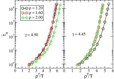
Figure 1. Breakdown of power-law density scaling for the reduced structural relaxation time  in the KABLJ mixture,
  , where τα is the time at which the self-intermediate scattering function (Fs(q,t), q = 7.25(ρ/1.2)1/3) for the A particles has decayed to 1/e. Molecular dynamics (MD) simulations in the NVT ensemble (N = 1000) were performed using RUMD, an MD package optimized for state-of-the-art GPU computing (see http://rumd.org). The time step was kept constant in reduced units,
  .
.
 is plotted for three isochores as a function of the density-scaling variable ργ/T, where γ is an empirical scaling parameter. Left panel: γ = 4.90 collapses the data for the two lowest densities. Right panel: γ = 4.45 collapses the data for the two highest densities. It is not possible to find a single exponent that collapses all the data; even though the two exponents differ by only 10%, power-law scaling with a single exponent clearly fails.
Download figure:
Standard imageWhat causes power-law density scaling and its breakdown for large density variations? A justification of density scaling may be given by reference to inverse power-law (IPL) potentials (∝r−n), where r is the distance between particles. For such unrealistic, purely repulsive systems, density scaling is rigorously obeyed with γ = n/3 [27]. Assuming that power-law density scaling reflects an underlying effective power-law potential, the scaling exponent γ can be found from the NVT equilibrium fluctuations of the potential energy U and the virial W = pV −NkT (IPL potentials have W = (n/3)U) as follows:

This was confirmed for the KABLJ mixture by Coslovich and Roland [23] and Pedersen et al [24]. Pedersen et al [24] further supported this 'hidden scale invariance' explanation by demonstrating that for the investigated density range the dynamics and structure of the KABLJ mixture are accurately reproduced by an IPL mixture with exponent chosen in accordance with equation (1).
The hidden scale invariance is not just a feature of the KABLJ mixture but of 'strongly correlating liquids' in general [28–31]. These are defined by having strong correlations between equilibrium NVT fluctuations of the potential energy and the virial (correlation coefficients larger than 0.9). Also molecular models can be strongly correlating; examples include the Lewis–Wahnstrom model of ortho-terphenyl and an asymmetric dumbell model. Both models are strongly correlating and obey power-law density scaling with exponents consistent with equation (1) for density increases of 8 and 16%, respectively [32]. Very recently, Gundermann et al [20] investigated the van der Waals liquid tetramethyl-tetraphenyl-trisiloxane, and gave the first experimental confirmation of the relation between the power-law density scaling exponent and equation (1).
For any potential that is not an IPL the exponent γ as calculated from equation (1) depends on the state point. Power-law density scaling corresponds to disregarding this state-point dependence. It is thus not surprising that power-law density scaling breaks down when large density changes are involved, but interestingly a more fundamental and robust form of scaling can be derived [33]. In the following, we proceed to derive the new scaling by a different route than used in [33].
Strongly correlating liquids have 'isomorphs' in their phase diagram, which are curves along which the structure and dynamics in reduced units are invariant to a good approximation [25, 26]. The invariance of structure implies invariance of the configurational ('excess') entropy, Sex; thus the isomorphs are the configurational adiabats. Gnan et al [25] discussed in detail the consequences of a liquid having isomorphs and also showed that a liquid is strongly correlating if and only if it has isomorphs to a good approximation. The precise definition of an isomorph [25] is that this is an equivalence class of state points, where two state points are termed equivalent ('isomorphic') if all pairs of physically relevant micro-configurations of the two state points, which trivially scale into one another, have proportional configurational Boltzmann's factors. From this single assumption several predictions can be derived, including isomorph invariance of structure and dynamics in reduced units and that jumps between isomorphic state points take the system instantaneously to equilibrium [25].
Letting R denote a micro-configuration (all particle coordinates) of a reference state point (ρ*,T*), the condition for state point (ρ,T) to be isomorphic with (ρ*,T*), i.e. the proportionality of pairs of Boltzmann's factors can, by taking the logarithm and rearranging, be expressed as

where K is a constant that only depends on the two state points. Equation (2) is the basis of the so-called direct isomorph check [25]: (a) draw micro-configurations R from a simulation at (ρ*,T*), (b) evaluate the potential energies of these configurations scaled to density ρ, and plot them in a scatter plot against the potential energies at ρ*. If a state point (ρ,T) exists that to a good approximation is isomorphic with (ρ*,T*), this scatter plot will be close to a straight line and the new temperature T is determined as T* multiplied by the slope.
In the following, we consider systems where the interaction potential between particles i and j is given by a sum of IPLs:

This includes the standard 12-6 LJ potential, but also, e.g., potentials with more than two power-law terms. We note that some systems interacting via equation (3) will not be strongly correlating and thus not have good isomorphs. In the following, properties are derived for those systems that do have good isomorphs.
The total potential energy of a given micro-configuration R at density ρ* is a sum over contributions from the power-law terms,  . When scaling R to the density ρ, keeping the structure invariant in reduced units, each power-law term is scaled by
  , and the potential energy at the new density
  is [26]

Thus, the linear regression slope of the U',U-scatter plot in the direct isomorph check is given by (where all averages refer to the reference state point (ρ*,T*))

Using Einstein's fluctuation formula for the excess isochoric heat capacity and the corresponding formula for the 'partial' heat capacities (which can be negative),

we obtain an expression for the new temperature T relative to the reference temperature T* (compare equation (2)):

Since  the number of parameters in the scaling function
  is one less than the number of terms in the potential (equation (3)). In particular, for the standard 12-6 LJ potential,
  contains just a single parameter:

Using that U12 = W/2 − U for 12-6 LJ systems [26],  can be conveniently expressed in terms of γ* defined as equation (1) evaluated at the reference density ρ*:

Equation (7) provides a convenient method for numerically tracing out an isomorph—previously this could only be done by changing density by a small amount, e.g. 1%, and then adjusting temperature to keep the excess entropy constant, using that γ (equation (1)) can also be expressed as [25]

It is a prediction of the isomorph theory that γ depends only on density [25, 26]. This means that the same differential equation, equation (10), determines the temperature on all isomorphs, implying that  is the same for all isomorphs—what changes between different isomorphs is T*. Thus
  is an isomorph invariant (compare equation (7)), which can be used as a scaling variable for the reduced relaxation time
  that is also an isomorph invariant [25]
  . This form of scaling was first proposed by Alba-Simionesco et al [14]. Here a theoretical derivation has been provided, as well as an explicit expression for
  for systems interacting via generalized LJ potentials (equation (3)).
What is the difference between the derivation presented here and the derivation presented in [33]? The derivation in [33] is thermodynamic in nature—from the invariance of excess entropy and heat capacity along the same curves in the phase diagram (the isomorphs) follows directly the general form of the scaling  In contrast, the derivation presented here is statistical-mechanical in nature—from the direct isomorph check (equation (2)) and the invariance of structure on isomorphs follows directly the specific form of the scaling for generalized LJ systems (equation (7)).
From the scaling  it follows that power-law density scaling is obeyed when considering only pairs of isochores: choosing one of the densities as the reference density, γ is uniquely determined so that
  where
where  is the other density divided by the reference density. Since the power law is then equal to
  at the two densities involved (
 , see equation (7)), it follows that the two isochores obey power-law density scaling with the exponent γ. This is indeed what is seen in figure 1. Choosing ρ* = 1.6 as the reference density, the scaling in the left panel of figure 1 corresponds to h(1.2/1.6) = (1.2/1.6)4.90 which via equation (9) leads to γ* = 4.59. Using this value we find that h(2.0/1.6) = 2.70 = (2.0/1.6)4.45. Thus from one power-law scaling exponent in figure 1, the other is uniquely predicted. Moreover, the value γ* = 4.59 is consistent with what is found by evaluating equation (1) at the reference isochore ρ* = 1.6 in the temperature range T = 1.7–5, which leads to values of γ* decreasing from 4.6 to 4.5. In the following figures reporting the results for the KABLJ mixture, we use γ* = 4.59 as estimated from the left panel of figure 1, i.e. no further fitting or adjustment of parameters was applied.
As mentioned, the scaling function  was derived assuming that good isomorphs exist. In figure 2 we test this for the KABLJ mixture using the most sensitive isomorph invariant—the dynamics of viscous states. State points with the same
  , predicted to be on the same isomorph, are seen to have very similar dynamics even though the density varies from 1.2 to 2.0.

Figure 2. Four different isomorphs in the KABLJ mixture, each generated from the condition  Densities range from 1.2 to 2.0, and
  (equation (9)) with γ* = 4.59 determined from the scaling in figure 1, see text (
 , ρ* = 1.6). (a) Self part of intermediate scattering functions in reduced units. (b) Mean-square displacements in reduced units. The data collapse confirms that true isomorphs have been identified.
Download figure:
Standard imageFigure 3 tests the proposed scaling for the KABLJ mixture using the data of figure 1. Clearly, the new form of scaling works well. Combining equation (10) with the definition of  (equation (7)) shows that γ is the logarithmic derivative of
  , γ = d ln h/d ln ρ. The inset of figure 3 demonstrates that this prediction agrees well with simulations even when going to large densities (where the purely repulsive r−12 limit is approached).
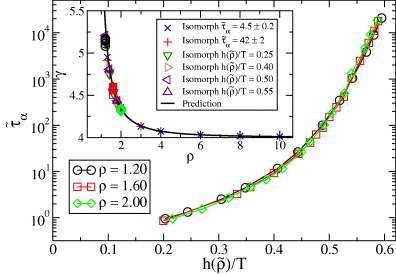
Figure 3. Reduced relaxation times for the KABLJ mixture scaled according to the isomorph theory (same data as in figure 1). The scaling function  is the same as in figure 2 (equation (9), γ* = 4.59). Inset: comparing γ computed from simulations (equation (1)) to the prediction of the isomorph theory, γ = d ln h/d ln ρ (black curve). Isomorphs denoted by a reduced relaxation time are each generated from a single reference point using equations (7) and (9), with ' ± ' quantifying the resulting variation of the reduced relaxation time on the isomorph. Isochores are plotted with the same symbols as in the main figure.
Download figure:
Standard imageWe now turn briefly to molecular models. In this case it is still a prediction of the isomorph theory that an expression of the form  is the right scaling variable [33], but we do not have an explicit expression for
  . Figure 4 demonstrates how power-law density scaling breaks down for the Lewis–Wahnstrom model of ortho-terphenyl and an asymmetric dumbell model when considering larger density changes than previously studied [32]. Like in figure 1, power-law scaling works when considering pairs of isochores, consistent with the right scaling variable being of the form
  . The insets of figure 4 test the isomorph prediction that γ to a good approximation is a function of density only, the assumption used to derive the new scaling. The prediction agrees well with simulations: γ is found to be much more dependent on density than on temperature. For more results on isomorphs in these model molecular liquids, see [34].
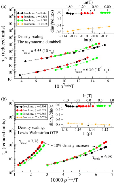
Figure 4. Breakdown of power-law density scaling in two molecular models. In accordance with the scaling derived in the present work, power-law scaling does work when considering only pairs of isochores. (a) The asymmetric dumbbell model. (b) The Lewis–Wahnstrom model of ortho-terphenyl (OTP). Insets: (∂ ln γ/∂ ln T)ρ plotted against lnT (circles) and (∂ ln γ/∂ ln ρ)T plotted against ln ρ (stars). Consistent with the isomorph theory, γ is found to be much more dependent on density than on temperature.
Download figure:
Standard imageFinally, we present in figure 5 a new analysis of experimental data for the two van der Waals liquids dibutyl phthalate (DBP) and decahydroisoquinoline (DHIQ), using larger density increases than usually studied in scaling experiments (20 and 18%, respectively). For DBP, dielectric relaxation times were taken from [35], and densities were calculated from the Tait equation of state [36] fitted to PVT data from Bridgman [37]. For DHIQ, dielectric relaxation times were taken from [38], and the Tait equation of state with parameters estimated by Casalini et al [39] was used to calculate densities. We find that the isochronal dependences log10 T versus log10 ρ determined at given structural relaxation times in reduced units,  , where vm and m are the molecular volume and mass, are nonlinear (figures 5(b) and (e)). This implies breakdown of power-law density scaling. The isochrones can be superposed after vertical shifting, however (figures 5(c) and (f)), which implies that a scaling variable exists of the form h(ρ)/T. The isochrones can be described by a phenomenological form of the scaling function log10(h)(ρ) = A1 log10 ρ + A2 log210 ρ, chosen here simply to take into account the curvature. Our results for DBP are consistent with those reported by Niss et al [41]. We conclude that for DBP and DHIQ, power-law density scaling breaks down at large density variations in the way predicted by the isomorph theory. Interestingly, the density dependence of γ is stronger than for the model systems and in the opposite direction; for the experimental systems γ
increases with density.
, where vm and m are the molecular volume and mass, are nonlinear (figures 5(b) and (e)). This implies breakdown of power-law density scaling. The isochrones can be superposed after vertical shifting, however (figures 5(c) and (f)), which implies that a scaling variable exists of the form h(ρ)/T. The isochrones can be described by a phenomenological form of the scaling function log10(h)(ρ) = A1 log10 ρ + A2 log210 ρ, chosen here simply to take into account the curvature. Our results for DBP are consistent with those reported by Niss et al [41]. We conclude that for DBP and DHIQ, power-law density scaling breaks down at large density variations in the way predicted by the isomorph theory. Interestingly, the density dependence of γ is stronger than for the model systems and in the opposite direction; for the experimental systems γ
increases with density.
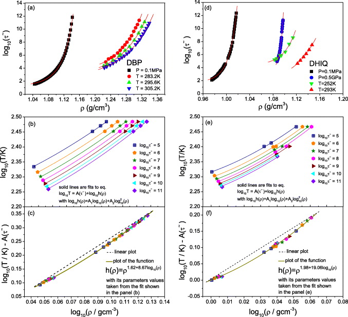
Figure 5. Deviation from power-law scaling in DBP ((a)–(c)) and DHIQ ((d)–(f)). (a) and (d) Density dependence of isobaric and isothermal structural relaxation times  in reduced units. Solid lines represent separate fits to the modified Avramov model [40]. (b) and (e) The isochronal dependences log10 T versus log10 ρ determined at a given
  . Fits are done to all isochrones simultaneously. (c) and (f) The isochrones vertically shifted by the fitted values
  . Deviations from power-law scaling (straight dashed lines) are evident. The fitted h(ρ)'s correspond to γ values increasing from 2.6 to 3.9 (DBP) and from 2.0 to 4.3 (DHIQ).
Download figure:
Standard imageWhat are the perspectives of our findings? Based on the theory of isomorphs in dense liquids we have now a form of density scaling that is more fundamental and more robust than power-law density scaling and which is consistent with both simulations and experiments. This 'isomorph scaling'—in its mathematical form originally proposed by Alba-Simionesco et al [14]—is predicted to apply for all strongly correlating liquids, i.e. van der Waals and metallic liquids, but not, e.g., for hydrogen-bonding liquids. Our results should not be used to abandon power-law density scaling—it is a useful approximation to isomorph scaling when the scaling function h(ρ) is unknown and only moderate density changes are considered. Under these conditions the isomorph theory predicts that power-law density scaling works with an exponent determined by equation (1). Isomorph scaling provides a deeper understanding of why—and when—power-law density scaling works.
An interesting perspective is to what extent isomorph scaling can be generalized to Brownian dynamics in colloidal or nanoparticle suspensions. A necessary—but not sufficient—condition is that the diffusion coefficient in appropriate reduced units [25] is a single-valued function of excess entropy, since these are both isomorph invariants. This condition rules out, e.g., the Gaussian core, Hertzian and effective star-polymer models [42]. On the other hand, it does leave open the possibility that, e.g., the Yukawa potential used to model charge-stabilized colloidal suspensions and complex (dusty) plasmas has isomorphs, and thus obeys isomorph scaling [43, 44].
Isomorph scaling has important consequences for the most fundamental open question in the field of viscous liquids and glass transition: what controls the dramatic viscous slowing down? In general, this question has to be considered as a search for a physically justified function of two variables, temperature and density (or temperature and pressure). Our results imply that this problem is now effectively reduced to a search for a function of a single variable, at least for the class of strongly correlating liquids. This is particularly striking for LJ-type systems such as the KABLJ mixture, where we have a prediction for the scaling function that agrees very well with simulations for much larger density variations than usually considered. The fact that the LJ scaling function contains just a single parameter—i.e. no more parameters than power-law density scaling—confirms that isomorph scaling is more fundamental and not merely a higher-order approximation compared to power-law density scaling. Isomorph scaling must be taken into account in theories of the viscous slowing down: since the relaxation time in reduced units obeys isomorph scaling, any quantity proposed to control the relaxation time must also obey isomorph scaling [25].
Acknowledgments
The Centre for Viscous Liquid Dynamics 'Glass and Time' is sponsored by the Danish National Research Foundation. AG and MP gratefully acknowledge support from the Polish National Science Centre (the project MAESTRO 2).