Abstract
Probing of micro- and nanoscale mechanical properties of soft materials with atomic force microscopy (AFM) gives essential information about the performance of the nanostructured polymer systems, natural nanocomposites, ultrathin coatings, and cell functioning. AFM provides efficient and is some cases the exclusive way to study these properties nondestructively in controlled environment. Precise force control in AFM methods allows its application to variety of soft materials and can be used to go beyond elastic properties and examine temperature and rate dependent materials response. In this review, we discuss experimental AFM methods currently used in the field of soft nanostructured composites and biomaterials. We discuss advantages and disadvantages of common AFM probing techniques, which allow for both qualitative and quantitative mappings of the elastic modulus of soft materials with nanosacle resolution. We also discuss several advanced techniques for more elaborate measurements of viscoelastic properties of soft materials and experiments on single cells.
Export citation and abstract BibTeX RIS
1. Introduction
Scanning probe microscopy (SPM) methods provide a variety of tools to access micromechanical properties by measuring the interactions of a sharp probe with the specimen surface.1,2) Precise control over the force applied to the probe allows one to study a variety of materials ranging from very compliant live cells to extremely stiff cellulose fibrils and rigid polymers.3–5) At the same time, the accuracy of modern piezo actuators provides the opportunity to perform these measurements with nanoscale precision and map inhomogeneous soft materials on the length scale of a single polymer chain.6) Furthermore, such force and spatial precision combined with current state of the art setups enabling image acquisition times on the order of seconds provides SPM-based methods with the unique ability to study changes in mechanical properties of nanostructured soft materials in real time in controlled environments. The measurements can be performed in liquid,7) controlled atmosphere,8) high vacuum,9) reduced or elevated temperatures.10) In addition the probe itself can be modified to mimic the properties of specific soft materials or decorated with cells and molecules to study adhesive behavior of different components of nanostructured systems.11)
In this review, we will briefly summarize advanced SPM methods currently utilized for micromechanical characterization of polymers and biomaterials. We will introduce the reader to the operating principles and discuss major advantages and disadvantages of presented techniques for specific applications. We will demonstrate the applications of these techniques for the simple characterization of the sample surface, advanced measurements of temperature and time sensitive mechanical properties, as well as imaging and characterization of biomaterials, bacteria, and cells.
2. Basics of SPM contact mechanics
In order to perform a measurement in all mechanical modes of SPM a sharp probe has to make stable physical contact with the sample surface. The system commonly consists of flexible cantilever with a sharp, microfabricated probe at its end which can be chemically modified in order to measure local forces (chemical force microscopy).12,13) Typically cantilevers are rectangular or V-shaped, however other shapes of cantilevers exist for specific applications.14–16) Cantilevers are usually made of single crystal silicon or silicon nitride and the back side of the cantilever (the side opposite to the tip) is coated with metal (usually gold, platinum, or aluminum) to increase reflectivity. In most of the current atomic force microscopy (AFM) setups the cantilever is attached to a piezo-actuating tube, which allows positioning of the tip over the investigational areas with a precision of about 0.1 nm [Fig. 1(a)].17) Additional piezo-actuators can be installed to the sample holder for advanced tip–sample interaction control. The main operational principle of all state of the art AFM systems is the measurement of the tip–sample interactions through detection of cantilever deflection. The most common way to monitor cantilever deflection is the so-called optical lever method: a laser is reflected from the metal-coated back side of the cantilever into a four quadrant photodiode [Fig. 1(a)]. Thus, this method allows separate measurements of the vertical (topography) and torsional (friction) deflection of the cantilever at high rates, with the maximum rates in the MHz range.18,19) The sensitivity of the photodetector to the applied forces depends on the shape and spring constant of the cantilever, which can vary in the 0.01–100 N/m range for most soft material applications.

Fig. 1. (a) Schematic of the common AFM setup. (b) Main regions of FDC as discussed in text. Young's modulus map of uncompatibilized POE/PA6: (c) (12 × 12 µm2) map, (d) zoom in to the interfacial regions (0.5 × 0.5 µm2). (b) and (c) reprinted with permission from Ref. 32. © 2010 American Chemical Society.
Download figure:
Standard image High-resolution imageDuring the measurements, the AFM tip raster scans across the surface of the sample providing a rectangular pattern with the information about sample topography and mechanical properties. Generally acquisition of the data for each point can occur either in the quasi-static or dynamic mode.20) In the next section, we will briefly discuss basic principles of these techniques and their applications for mechanical surface characterization.
3. AFM methods for elastic properties measurement
3.1. Quasi-static loading
Historically, the first developed mode for mechanical measurements involved quasi-static loading of the sample surface.21) In this mode AFM tip is brought into the contact with the sample, is pressed against it, and then withdrawn. The full approach-retract cycle is presented schematically in [Fig. 1(b)] and consist of the several major regions: 1) the tip is far away from the sample with no forces exerted on it; 2) the tip first touches the sample (contact point); 3) the tip is positively deflected when pressed against the sample; 4) the tip is negatively deflected by the attractive forces during the retraction portion of the loading cycle prior to loosing contact with the surface. The forces calculated from the tip deflection can be plotted against the actuator position to achieve so called force–distance curves (FDCs). Application of various contact mechanics models to the different regions of recorded FDCs allow for calculation of mechanical properties such as elastic modulus and adhesion as briefly summarized below.22)
In the simplest case, Sneddon's contact model is applied to the tip–sample interaction.23) In this model the tip is represented by the axisymmetric rigid punch indenting into the elastic half space. For common tips and low indentation depths, a parabolic tip shape is usually assumed.27) For the analysis the FDC is transformed into a force-penetration curve, where the force F is calculated from the deflection of the cantilever (d) and the spring constant of the cantilever (k) as  , and penetration δ is calculated through the difference between the relative piezo displacement (z) and cantilever deflection (d) as
  . From the force-penetration curves elastic modulus can be calculated as27)
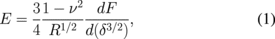
where R is the radius of the curvature of the apex of the tip and ν is the Poisson's ratio of the sample material. Over the years more complicated contact mechanics models were developed to consider the effect of tip shape, sample roughness, adhesive behavior, and electrostatic properties on the mechanical characterization of the samples with quasi-static FDC collection.24–27)
AFM imaging by FDC collection in each point of the sample is frequently called Force–Volume (FV) imaging mode. FV imaging allows for quantitative mapping of regions of different mechanical behavior on the nanoscale and has been used to characterize polymer blends, grafted polymer brushes, proteins and nanopatterned polymer structures.28–31) For example, Wang et al. employed FV imaging to study compatibilization between polymers in polymer blends32) and FV was applied to study microthermal properties of polymer blends.33) Figures 1(c) and 1(d) show modulus maps acquired the Johnson–Kendall–Robert (JKR) model for adhesive contact, of an uncompatibilized and a reactive compatibilized blend of polyolefin elastomer (POE)/polyamide (PA6).
Because the surface deformation and forces can be controlled using the FV method, the elasticity of ultrathin and multilayered thin films, which are not accessible via any other techniques, can be studied with the application of simple layered contact mechanics models.34–36) Furthermore, the pull-off point of the retract curve [Point 4 in Fig. 1(b)] can be used to map adhesive properties of the surface, which was used in numerous applications.37,38) Despite its usefulness, there are however several pitfalls to this technique. The first one is related to the assumptions of chosen contact mechanics model. These contact mechanics models are usually applied for simple indenter shapes (such as paraboloid, sphere, cone, and pyramid), and the nanoscale dimensions of AFM-based measurement can strongly influence calculated elastic properties. Thus, to perform quantitative calculations, the tip shape should be precisely characterized. This can be done by scanning electron microscope (SEM) imaging, topography reconstruction,39) or indentation into the sample with the known modulus.40) The other assumption of the simple contact mechanics models is ideally flat sample topography. Therefore sample roughness plays a role in measurements precision, as well as selection of valid regions for measurements.41) Cantilever stiffness is another important parameter directly related to the elastic measurement precision: for high signal to noise ratios in FDCs the stiffness of cantilever should be close to that of the measured material.42)
Another important issue of the FV mapping is related to the fact that a single measurement is performed at a constant indentation rate and this rate is limited by the nonlinearities of piezo-actuator extension.43) Therefore, mapping with this technique can take a considerable amount of time and can be impractical for real time applications. Even if sample stability is not the issue, the limitation of the measurement rate brings out the problem of AFM stability over the course of the measurements. Over the years of the development of FV several works have been published which discuss the shortcomings and operational procedures of this technique in detail.26,44,45) To improve these drawbacks dynamic measurement modes were developed.
3.2. Dynamic methods
In dynamic methods high frequency vibrations are applied to the tip–sample contact through the actuation of the cantilever, the sample, or both. Cantilever response is then measured in different regions of the sample in terms of parameters of the vibrations (such as amplitude, phase or frequency changes) to collect contrast maps and quantitatively calculate the elastic properties of the material. Here, we will focus on several common dynamic techniques grouped by their principle of operation.
3.2.1. Tapping mode
In tapping mode, voltage is applied to the tip at a frequency close to its resonance and intermittent contact with the sample is performed. The reduction of the tip–sample contact time allow for reduction of lateral forces, which appear during the tip motion across the scanned surface.46) Typically tapping mode is performed in amplitude modulation mode: the height of the cantilever position is constantly adjusted to keep a constant ratio of the tip vibrational amplitude in contact with the sample surface to its oscillation amplitude in air, thus imaging topographical features of the sample. The phase shift of the vibrations relative to the excitation vibrations bears information about the energy dissipation by the tip into the sample. The phase imaging technique can be used to produce excellent material contrast, especially in systems with close mechanical properties, without any additional post processing of the measurement data.47) Due to the fact that forces between the surface and the tip are not measured directly in tapping mode, this technique does not allow for quantitative measurements of the elastic modulus of the material. However it was shown that it can be used to perform contrast variation in some cases of hard tapping in multi-component rubbers and binary brushes.48–50)
3.2.2. Force modulation microscopy
In contrast to tapping mode, force modulation microscopy measurements (FMM) are performed in contact mode. The cantilever is displaced vertically to maintain constant deflection while the tip scans across the surface thus mapping the sample topography, while at the same time the cantilever is vibrated at a frequency which is much lower than the resonance frequency, but is still high enough to avoid distortions due to the instrument resonance. During these vibrations the tip stays in the repulsive contact regime with the sample surface, therefore simplifying the tip–sample interaction forces compared to tapping mode, where transitions between attractive and repulsive modes may occur.
Simple analysis, therefore, can be applied to the system under the assumption of elastic material behavior.51) In this analysis the tip is assumed to be attached to the piezo-actuator with the spring with the stiffness kc. At the same time the tip is considered connected to a spring with the stiffness ks, which represents the elastic sample. The tip–sample vibrational amplitude u can be then described as52)

where ω is the angular frequency of induced vibrations, and u0 is the drive amplitude of the vibrations. Since the contact area is unknown, only tip–sample contact sample stiffness can be calculated. As an example, this method was used to map the elastic properties of micropatterned, end-tethered proteins on gold (Fig. 2).53) The relative modulus can be acquired as well by using a calibration sample with well-known elastic properties.54,55) It is important to note that the simple elastic model presented here is not applicable in the case of nonlinear responses and more complicated analysis should be used.56)
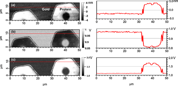
Fig. 2. FMM images of staphylococcal protein A domains for IgG-binding (SpA-N B) patterns on a gold surface, with corresponding cross-section analysis along the red line in the AFM images in (a) topography, (b) amplitude, and (c) phase channels. Reprinted with permission from Ref. 53. © 2012 Beilstein-Institut.
Download figure:
Standard image High-resolution image3.2.3. Contact resonance AFM
In contact resonance AFM (CR-AFM), similar to the FMM, scanning is performed in the contact mode and cantilever is excited dynamically in high frequency range at relatively low amplitude. However, as the name suggests, in CR-AFM vibrations of the tip are kept close to the resonance frequency of the cantilever.57) Similar to the FMM, during the contact with the sample in CR-AFM tip behavior changes relative to its free vibrations. The resonance frequency of the vibrations shifts, which could be mathematically described by additional spring attached to tip when it is pressed against the surface. This spring describes the stiffness of the sample and would shift the resonance frequency of the cantilever to higher value. AFM cantilevers have several resonant frequencies, which are related to the flexural eigenmodes of the cantilever.58) Higher modes of cantilever vibrations are excited at much higher frequencies (usually in MHz range) and increase the overall stiffness of the cantilever. CR-AFM utilizes this feature and can be executed in different vibrational modes depending on the substrate stiffness, which increases the range of the materials which can be characterized with the same tip. Most of the current configurations do not have the capability to induce contact vibrations at such high frequencies, therefore for CR-AFM at higher eigenmodes additional actuators are required. In addition, the photodiode should be able to accommodate for the high frequency tip deflections.59)
The CR-AFM method can be utilized in different ways, depending on the application. The simplest way is to perform qualitative imaging, which is executed by keeping the vibration frequency constant and monitoring the change in amplitude as the tip scans the sample. The contrast of the image can be tuned by the changes of the oscillation frequencies around the resonance peak or by switching to different vibrational modes. For example, qualitative imaging was performed on self-assembled monolayers (SAMs) of n-octyldimethylchlorosilane in varying humidity.60) In this case CR-AFM amplitude imaging provided much higher contrast than other measurement methods due to its insensitivity to the humidity effects, such as capillary bridge formation between the tip and the sample surface. This technique is also useful for measurements of stiff crystalline polymers and polymer composites. For example, it was used for poly(3-hexylthiophene) (P3HT) blended with the fullerene derivative phenyl-C61-butyric acid methyl ester (PCBM) to provide high contrast between crystalline and amorphous domains.61)
Another mode of operation of CR-AFM is a spectroscopic mode. In this mode, the vibration amplitude is recorded for the range of vibrational frequencies, establishing the full shape of the resonance curve. Knowing the resonance frequency allows one to apply analysis similar to the one discussed in the FMM method to calculate stiffness of the tip–sample contact.62) This spectroscopic analysis can be performed in the CR-AFM mode as well, where a full frequency range sweep is performed at each point. This method is time consuming; therefore several improved methods of resonance frequency detection have been developed. For example, it is possible to track the position of the resonance peak by keeping the frequency window close to each previous resonance position for each subsequent point.63) The other method relies on dual AC resonance tracking (DART) method where two separate vibrational frequencies are applied to the system.64) The frequency controller is constantly adjusting these frequencies to achieve the same amplitude response for both, therefore positioning the resonance frequency value as an average between the two values. CR-AFM elastic mapping was applied to polymer blends, as it produces qualitative elastic data with enhanced contrast compared to the simple tapping mode.65) Some of the drawbacks of this technique include the limited ability to measure very soft samples due to the contact operation regime and difficulties of quantitative measurements in liquid.66)
3.2.4. Ultrasonic AFM
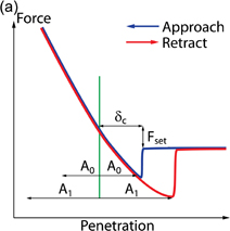
The ultrasonic AFM (UAFM) technique is similar to FMM and CR-AFM in that a tip is constantly pressed against the sample surface and vibrations are induced into the tip–sample contact. There are however two major differences in the UAFM approach: 1) the applied frequency is much higher than the natural resonance frequency of tip vibration; and 2) the amplitude of this frequency is constantly changing, while the average tip deflection is monitored.67) The concept of UAFM operation is presented in Fig. 3. Initially, when the vibration amplitude is low, the average tip deflection stays constant. When the vibration amplitude reaches A0 the deflection starts increasing nonlinearly, indicating that the tip has reached the attractive regime of tip–sample interaction. At an even higher amplitude, A1, the tip fully detaches from the sample producing a noticeable increase in the average cantilever deflection (Fig. 3). This threshold amplitude A1 is used in UAFM as the parameter to map the stiffness distribution of the sample surface: for more compliant material initial penetration δc would be higher, and therefore would require higher threshold amplitude. Due to the complexity of the tip–sample interaction only contrast imaging reflecting the stiffness of the components can be recorded.
Download figure:
Standard image High-resolution image
Fig. 3. (a) Typical UAFM measurements parameters on FDC. (b) Amplitude change at each point in UAFM experiment. (c) Corresponding average forces acting on the tip.
Download figure:
Standard image High-resolution imageDue to the tip–sample stiffening at high vibration frequencies, UAFM can be used to study materials in the wide (1–400 GPa) modulus range. It was applied to study polymer blends, nanocomposites with high variation of component stiffness, and thin films. However, the technique is well suited for measurements of viscoelastic samples, which change their properties at ultrasonic frequencies and materials with high variations in adhesive properties and roughness.66)
3.2.5. Pulsed force imaging
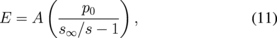
In pulsed force imaging the tip contacts the sample during the down portion of a sinusoidal vibration cycle (Fig. 4).68) Each cycle starts above the surface, then the tip approaches and makes brief contact with the surface resulting in a small indentation. The depth of this indentation is controlled by the maximum force exerted on the sample by the cantilever (set point). The cycle is finalized by withdrawing the tip from the surface up to the initial baseline static deflection. By limiting the set point, indentations as small as 1–2 nm can be performed, therefore achieving very soft, nondestructive measurement conditions. Approach and retract FDCs can be reconstructed from the loading data (Fig. 4); however the analysis of these curves differs from quasi-static measurements. Because of the low calculation time requirements for real time analysis in pulsed force imaging, the set point force (Ftip) and adhesive force (Fadh) are used instead of the full curve fitting to calculate elastic modulus according to the Derjaguin–Muller–Toporov (DMT) model as5)
Further analysis of the FDCs allows for simultaneous measurement of adhesion and energy dissipation in addition to the sample topography and elasticity.

Fig. 4. (a) Variation of the force as a function of time in a pulsed force imaging experiment: experimental curve (solid line) and constant tip sample contact case (dashed line). (b) Corresponding cantilever displacement. (c) FDC reconstructed from the approach and retract portions of the loading curve presented in (a).
Download figure:
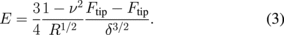
Standard image High-resolution imagePulsed force imaging allows acquisition of high resolution qualitative maps of mechanical properties of the sample both for dry samples and in liquid. This technique was successfully applied to various polymers69,70) and biomaterials.71–73) For example, this mode was explored to characterize structural regions with different mechanical properties in soft silicone-hydrogel lenses.74) In this work, contrast imaging with quantitative nanomechanical property mapping was performed via Peakforce QNM in liquid and the mechanical properties of the various regions of the lens were then acquired with quasi-static indentations at much lower loading rates (Fig. 5).
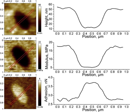
Fig. 5. Peak Force QNM imaging for complex composition of Balafilcon A contact lens material performed in three channels: topography, DMT modulus and adhesion. Reprinted with permission from Ref. 74. © 2014 Elsevier.
Download figure:
Standard image High-resolution imageIt is worth noting that the mechanical properties acquired with pulsed force imaging can deviate significantly from quasi-static measurements due to such effects as the apparent stiffening of the sample at high loading rates, nonlinear loading effects, and for materials with behavior strongly deviating from DMT model.26) Recently, Stan and Gates presented improvements of some of the shortcomings of the pulsed force imaging.75) It was shown that application of overlaying independent high frequency resonant vibrations to the PeakForce mode can facilitate the elastic modulus calculations. This calculation was done by resolving adhesive response of the material through Swartz adhesive model,76) allowing one to pick adequate adhesive behavior in between long range (DMT) and short range (JKR) models.
4. Viscoelastic properties measurements
Although mapping of elastic properties of soft materials provides critical information about materials performance it gives only a snapshot of the material behavior in the time–temperature domain at particular frequency. It is well known that relaxation processes in soft materials delay the response to external stress.77) This viscoelastic behavior is especially prominent around transition temperatures, such as the glass transition temperature in polymer systems, where the storage modulus of the material can change by more than 3 orders of magnitude.27) Therefore, it is important to take into account relaxation processes in the material as well as the rate and time dependence of these processes during mechanical AFM measurements. In this section, several currently employed approaches used for viscoelastic materials testing with AFM will be discussed along with examples of applications of these approaches.
4.1. Static creep test
In static creep tests the AFM tip is driven into the sample up to a set cantilever deflection, producing indentation force, F. Deflection is then kept constant by the feedback loop by moving the cantilever base to compensate for tip motion as the sample surface relaxes. Under constant load, creep of the loaded material can be observed and the penetration of the tip into the material can be analyzed using simple viscoelastic models which describe the material as an idealized set of springs and dashpots connected parallel or in series.78) Parameters of the model can then be calculated from fitting penetration with simple Sneddon's contact mechanics considerations for parabolic tip shape as78)

However this method has several drawbacks, most of which are related to the much extended times needed for the experiment. For long measurements piezo creep and high and changing signal noise can become an issue for precise curve fitting. As a result, regular mapping of viscoelastic properties becomes impractical. Therefore such measurements are often conducted for single point measurements. Additionally, fitting the curve with multiple unknown parameters can produce large fitting errors, so some constants need to be independently calculated with other methods.79) For example, Braunsmann et al.80) employed a preload step to creep test measurements of epoxy adhesive to purposely induce plastic deformations, therefore improving the control over the tip–sample contact shape and reducing plastic deformation on the main loading step, thus effectively reducing the number of unknown parameters of viscoelastic model.
4.2. Measurements at constant loading rate
A more elaborated approach for viscoelastic properties measurements utilizing AFM indentations was recently introduced, where instead of constant load application, viscoelastic properties were calculated for FV measurements performed at the constant loading rate.27) The modeling in this method incorporates use of creep compliance function for SLS material together with Sneddon's contact mechanics [Fig. 6(a)] to describe the penetration δ over time t as

where U is the sample loading rate, T is total loading time, τ is the relaxation time and E0 and E∞ are the instantaneous and infinite moduli of the SLS material, which describe material compliance in response to instantaneously-applied and infinitely-long loads respectively. Fitting experimental data with Eq. (5) allows for calculation of unknown SLS parameters (τ, E0, and E∞) at given experimental conditions.
Fig. 6. (a) Tip–sample interaction model for SLS material. (b) Storage E', loss E'' moduli, and loss tangent E'/E'' calculated for PnBMA material and simple elastic modulus E calculated for the same loading data through Sneddon's model. (c) Storage modulus and (d) loss modulus of the epicuticula layer of viscoelastic pad of Wandering spider. Panels (a) and (b) reprinted with permission from Ref. 27. © 2014 American Chemical Society. (c) and (d) reprinted with permission from Ref. 81. © 2014 Elsevier.
Download figure:
Standard image High-resolution imageBy varying loading rate and surface temperature one can calculate such properties of the material as temperature dependence of loss and storage moduli and relaxation times. Figure 6 shows results of such reconstruction for model poly(n-butyl methacrylate) (PnBMA) material. In addition to storage and loss moduli, this reconstruction contains data for simple elastic modulus estimation from FDCs for the same material. It can be seen that the apparent simple elastic modulus calculated through Sneddon's approach deviates strongly from actual storage modulus, especially at the maximum of the loss tangent, where the difference is more than two fold. Since this method utilizes regular constant rate indentations, it can therefore be applicable for the same instrumental conditions as simple FV mapping. For example this technique was used to examine a vibration transducing organ of wandering spider [Figs. 6(c) and 6(d)].81) In this work, loss and storage moduli variations of the thin epicuticular layer of the vibration transducing pad were related to the spiders' activity cycles and sensitivity to high frequency signals.
It is worth noting that fitting the penetration curves for these constant loading experiments can be challenging, especially under the conditions in which the material exhibits long relaxation times (e.g., elevated temperatures), which requires very slow loading rate to observe viscoelastic behavior. In such cases, high signal to noise ratios can significantly decrease precision of the fitting.
4.3. Acoustic methods
As was discussed above CRFM and FMM are similar AFM methods, which relate difference between free vibrations of the tip and the vibrations of the tip in contact with the sample to estimate elasticity of tip–sample contact. For viscoelastic materials with characteristic relaxation times near the timescales of the driving frequency, contact mode oscillations will be damped, providing a way to study loss properties of these materials. An important feature of all acoustic methods is constant contact of the tip with the sample, which reduces the routes of the energy dissipation almost exclusively to viscous contributions of the sample. This is in contrast to intermittent contact modes, where additional processes such as surface energy hysteresis, capillary bridge formation, and friction effects may occur.82)
Therefore, in the FMM mode, storage and loss properties of materials can be qualitatively mapped for viscoelastic materials with the elastic properties related to the amplitude and variation of contact stiffness and loss properties related to the phase shift of the tip vibrations.83) The quantitative values can be obtained from FMM measurements if, in addition to amplitude and phase values, simple elastic properties of the material are estimated with additional techniques.84) Since FMM methods can be applied through wide range of oscillation frequencies, this method is well suited for reconstruction of master curves of materials behavior. For example Nguyen et al. applied a modified FMM method with initial set point deflection achieved through the regular FV approach to create high quality maps of loss tangent for styrene-butadiene rubber (SBR)/isoprene rubber (IR) blend.85) It was shown that FMM methods show lower loss tangent values than the intermittent tapping mode, since the latter includes non-viscous energy dissipation.
CRFM does not have the advantage of the broad frequency sweeps of the FMM mode; however it can utilize several frequencies of different eigenmodes of the cantilever. Considering dynamic tip–sample interactions, relatively simple equations can be used to quantitatively calculate reduced storage  and loss
  moduli through some calibration material with known properties:86)
where ω is the resonance frequency, α and c are coefficients related to the tip geometry, and the subscripts "s" and "ref" stand for the sample and reference material, respectively. The method therefore can be effectively used to map the ratios for loss and storage moduli of polymer blends with high accuracy and speed.87) One of the useful features of the CRFM measurements is the lack of necessity for exact match between the stiffness of the cantilever and the substrate, since the selection of different eigenmodes can be used for tuning the sensitivity of the technique for the particular material.59) For measurements of the loss tangent, CRFM can provide quantitative data without relation to the reference materials. The method has been applied to multiple component polymer blends and bone–cartilage interfaces.88,89) The temperature variation during the measurements allows for reconstruction of master curves for evaluation of loss tangent and glass transition temperature.90)
4.4. Multifrequency AFM measurements
Long ago it was noted that the phase shift of the vibrations in the amplitude modulation setup can be related to the energy loss by the cantilever through the dissipative processes in the tip–sample contact.91) As it was discussed above, tapping mode cannot provide quantitative modulus measurements due to the complicated tip–sample interactions. To enable calculation of the elastic properties it was suggested to excite the cantilever at additional flexural modes.92) It was shown that if the second mode is excited at much lower amplitude than the main tip vibrations, the tip–surface interactions are strongly repulsive, which facilitates elastic properties estimations.
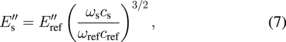
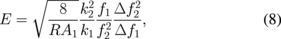
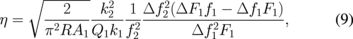
In bimodal AFM two flexural modes of the tip vibrations are excited at their resonant frequencies.93) It is important to note that both vibrations are excited and controlled by two separate feedback loops (Fig. 7). In this setup, lower frequency vibrations are performed in the amplitude modulation mode at amplitude, A1, while the lower amplitude, A2, additional vibrations are performed in frequency modulation mode (AM–FM configuration).94) Therefore it is possible to extract simultaneously four parameters of both modes simultaneously: frequency shift and amplitude for both vibrations, which can be denoted as Δf1, Δf2, F1, and F2. In this case mechanical parameters of the tip–sample contact such as reduced elastic modulus E, viscosity η and penetration δ can be calculated as95)
where k1 and k2 are the effective spring constants of the vibration modes, Q1 is the quality factor of larger amplitude vibrations, and R is the tip radius. This method therefore allows one to directly relate stiffness of the material to the frequency shifts of the second low amplitude mode in contrast to the simple tapping mode.93) At the same time, this method provides a way to quickly and reliably map viscoelastic properties polymer surfaces. For example Herruzo et al. showed the possibility of reliable viscosity and modulus mapping with bimodal AFM, observing granular structures within PS in PS-b-PBMA blend samples with domain sizes as low as 10 and 17 nm.95) The method has a great range of measured elastic moduli, for example it was used for mapping mechanical properties of proteins and the surface of mica, where the mapped modulus values span more than 3 orders of magnitude.96) There exist more elaborate methods of multifrequency measurements, where more than two flexural modes of the cantilever are used simultaneously. For example, Ebeling et al. used three eigenmodes to study the possibility of sub surface imaging.97) Figure 8 shows how the increase in the amplitude of the third eigenmode allows for imaging sub-surface structures with high lateral resolution. Overall, multifrequency AFM methods utilize simplified tip–sample interaction models and are more instrumentally demanding than any other AFM techniques. However, due to its applicability to a wide range of soft materials in different environments (ultrahigh vacuum, air and liquid) it is currently emerging as important practical approach.98)
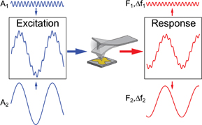
Fig. 7. Multifrequency AFM measurement principles.
Download figure:
Standard image High-resolution image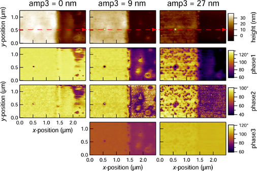
Fig. 8. Multifrequency measurements of the PDMS sample revealing silica particles in the sub-surface layers at higher amplitudes of the third vibrational mode. Reprinted with permission from Ref. 97. © 2013 American Chemical Society.
Download figure:
Standard image High-resolution image5. Application to investigate live cell mechanics
5.1. Elastic and viscoelastic nanomechanical properties of cell surfaces
Due to its excellent force sensitivity (10−12–10−9 N), and the ability to make measurements in physiological media at relevant temperatures, AFM quickly became an excellent tool in the field of cellular biomechanics, with the first AFM imaging of living cells being reported as early as 1991.99) Early experiments produced mappings of the elastic modulus of cellular surfaces, which are known to have important implications for many dynamic physiological processes, and can be used a potential diagnostic parameter for many serious diseases.100–103) A famous example is SFS on live metastatic cancer cells, which were successfully differentiated from healthy cells based on the estimated elastic modulus.104,105) Using standard Hertzian contact mechanics, it was found that cancerous cells displayed elastic modulus values approximately 73% lower than normal cells (∼0.5 kPa for cancer cells versus ∼2 kPa for normal cells). Surface elasticity measurements have also been conducted on bacterial samples to understand the cell response to varying environments, including low/high pH,106) exposure to antibiotics,107) and infection with bacteriophages.108)
General force spectroscopy measurements such as those described above serve as an excellent starting point to examine the structure-function relationship of the cell surface. However, the incredibly complex structure of living cells, which generally consists of several membrane layers and a cytoskeleton encapsulating a fluid environment (each of which has some associated viscous contribution) renders the assumption of linear elastic behavior somewhat inaccurate. Therefore, much effort has been focused on precise mechanical measurements to determine the viscoelastic behavior of single cells in physiological environments. For example, Rebelo et al. calculated elastic moduli and apparent viscosity using standard quasi-static indentation as described above.109) Here, the apparent viscosity was calculated from the work done by the viscous force from an approach/retract cycle which is revealed in the FDC hysteresis. Other investigations of the viscoelastic properties of cells have used some of the methods described in detail above such as static creep110) and amplitude-modulation.111)
An interesting measurement for live cell viscoelastic mechanical properties was described by Canetta et al.112) In this study, a colloidal bead was coated with specific binding antibodies and lowered onto a live cell until contact was made. After sufficient cell-probe binding had occurred the cantilever is raised at a constant rate, stretching the cell membrane and cytoskeleton upwards. The force was monitored as a function of time and was fitted with equations developed by Verdier and Piau113) for the viscoelastic properties of adhesive tack. While this method isolates the cell membrane/cytoskeleton and avoids the viscous contributions of the underlying nucleus, it is highly impractical for mapping and high throughput measurements. Additionally, force sensitivity is lost due to the use of a high resolution camera as a means to monitor cantilever deflection, rather than the usual optical method. In general, all of the methods discussed here serve as reasonable starting points to probe the viscoelastic mechanical properties of living cells. However the field is still relatively young, and as more is understood about cellular biomechanics, these AFM-based techniques will inevitably become more advanced as well.
5.2. Scanning ion conductance microscopy
In contrast to many of the methods described above, scanning ion conductance microscopy (SICM) utilizes an ion current in order to image sample surfaces.114) In these experiments an electrolyte-filled nanopipette, typically formed by drawing a heated glass capillary (opening diameter ∼100 nm), raster scans across a sample surface submerged in an electrolyte bath [Fig. 9(a)]. Voltage applied between electrodes located inside and outside cause ion current flow through the nanometer-sized aperture. This current flow is sensitive to blockages of the aperture, for example caused by close proximity to the sample surface, and thus can be used for topographical imaging.114–116) Because SICM is truly a noncontact method, it can be advantageously utilized to scan extremely fragile live cell surfaces.114) For example flexible microvilli, which are generally troublesome to image with traditional AFM approaches due to the mechanical interactions with the tip tending to drag the microvilli in the direction of the scan, were imaged successfully with good resolution (on the order of the inner tip radius115)).114,117) The non-contact mode of operation also significantly reduces the risk of tip contamination and when probing the elastic modulus (as discussed below), no assumptions need to be made about adhesive interactions between the probe and the surface.114)

Fig. 9. (a) The basic SICM set up for topographical imaging and modulus mapping. (b) Finite element model depicting the change in pressure as the ion solution is forced out of the nanopipette and the associated sample deflection. (c) Example current vs z-displacement curve used for elastic modulus calculation. (d) Panel showing fluorescent intensity, SICM topography, and calculated elastic modulus for a living fibroblast cell. Reprinted with permission from Ref. 116. © 2013 American Chemical Society.
Download figure:
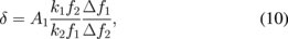
Standard image High-resolution imageElasticity measurements can be made with a SICM setup by applying a pressure to the upper end of the nanopipette and measuring the resultant ion current as a function of z-displacement [Fig. 9(b)]. Lowering the probe onto a stiff surface causes a much quicker drop in measured ion current compared to that of a soft surface, due to the ability of the surface to deform, Figs. 9(b) and 9(c). Finite element analysis was used to derive a simple relationship between elastic modulus and the slope of a current versus z-displacement curve taken between 99 and 98% of the maximum ion current, s:118)
where A is a constant associated with the tip geometry, s∞ is the slope for an infinitely stiff sample, and p0 is the applied pressure. Figure 9(d) shows a cell which was simultaneously mapped for topography and elastic modulus using SICM. Typical applied pressure can range from ∼0.1–100 kPa, resulting in a range of experimentally detectable elastic modulus values from ∼0.01–1000 kPa118) which is much better than usual range of on the order tens of kPa.119) However, despite its excellent applicability for imaging topography and stiffness of extremely soft surfaces, SICM is still in its infancy as far as wide-spread use. This is most likely due in large part to the environmental confinement to ionic solutions and the relative lack of commercial availability. Furthermore, quantification of data may require cumbersome numerical analysis.
5.3. Single-cell force spectroscopy
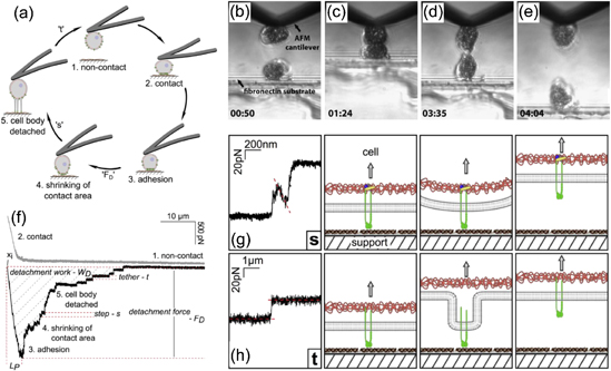
Cellular adhesion to surfaces (both host cells and invasive bacteria) controls many biological processes including inflammation and wound healing, infection, inter-cellular communication, tumor growth and metastasis, amongst others.120,121) As its name suggests, single-cell force spectroscopy (SCFS) involves attachment of a living cell to an AFM cantilever, effectively turning the cell into a probe [Fig. 10(a)]. From this, important adhesive behavior of a cell can be probed, including cell–substrate binding for implantable biomaterials,120) cell–cell interactions [Figs. 10(b)–10(e)],122) or cell interactions with specific binding proteins.123)
Fig. 10. (a) Set-up for a single loading unloading cycle in SCFS. (b)–(e) Optical image of a cell-on-cell SCFS testing. (f) Typical SCFS unloading curve with characteristic jumps (referred to as snaps, s, here) and tethers (t). (g) and (h) Schematic depiction of the different processes occurring during force jumps (g) and tether formation/breakage (h). (a), (f)–(h) reprinted with permission from Ref. 123. © 2013 Elsevier. (b)–(e) reprinted with permission from Ref. 122. © 2014 Elsevier.
Download figure:
Standard image High-resolution image
The first step in SCFS is attachment of a live cell onto a tip-less cantilever (or in some cases a functionalized colloidal probe), which has been functionalized with a cell-adhesive coating.124) The cantilever functionalization procedure will depend strongly on the type of cell to be measured, and the expected adhesive forces during the SCFS experiment.120) For example, gentle attachment of animal cells can be achieved via adsorption of lectins such as concavalin A or wheat germ agglutinin, or the use of receptor–ligand specific interactions with ECM proteins such as fibronectin.120,121,123) When much higher cell-detachment forces are expected, more elaborate approaches must be used, which utilize electrostatic interactions, hydrophobic interactions, or chemical fixation.124) Regardless of cantilever functionalization approach, one must be cognizant of the possible negative effects that the adhesive coating may have on the cell, including activation of cellular processes. The functionalized cantilever is then positioned above the selected cell and gently pushed into it for long enough to allow for sufficient adhesion to the cantilever (several seconds to minutes). The cantilever is then withdrawn from the surface and the cell is allowed to further attach more firmly to the cantilever. The cell attachment process is greatly facilitated by the use of one of many commercially available inverted optical microscope/AFM combinations.
Cell–substrate adhesive interactions are then quantified by collecting FDCs on desired surfaces [Fig. 10(a)]. Typically, the cell is pushed into the surface until a pre-determined force is reached (typically hundreds of pN), and then held for a predetermined time (on the order of fractions of a second to minutes). Applied force during the approach phase and contact time can heavily influence contact area (via cell spreading), therefore to produce consistent results it is highly desirable to monitor cell shape during measurement.123) Furthermore, contact time determines how many adhesive bonds the cell can form with the substrate, so typical experimental procedures involve using several prescribed contact times.120,123) The cellular probe is then retracted until the cell if fully detached from the substrate and some holding time (no shorter than the cell–substrate contact time) is given to allow for cell recovery before the next loading cycle is undertaken. In some cases, specialized hardware may be needed for soft cells (typically mammalian cells) which can require z-movement on the order of 100 µm for full detachment.120,121,123)
Retraction curves exhibit characteristic complex behavior, which is composed of both specific and non-specific interactions which can be analyzed separately [Fig. 10(f)].123) The maximum adhesive force is typically used as a general measure of cell adhesion. Similarly, the work of adhesion, or the area between the zero force level and the retract curve is used to characterize cell adhesion. The work of adhesion is strongly influenced by cell elasticity and the number of specific interactions formed during contact. As the force returns to zero, two discrete force events can be observed. Force jumps and non-linear increases in adhesive force represent the breaking of individual receptor–ligand bonds [Fig. 10(g)]. Another event, so-called membrane tethers, occur as a single cell surface receptor and membrane are pulled away from the cell surface forming few nm-diameter tubes [Fig. 10(h)]. The force required to extend a tether (which is a function of membrane mechanical properties) is constant and is seen as a plateau in the FDC, which decreases in a step-wise manner as tethers are broken.
No current procedures allow for the quantitative elucidation of single-cell adhesion forces with the pN–nN precision other than AFM-based SCFS. Current efforts are focused on increasing throughput as well as quantitatively separating the specific adhesion events from non-specific interaction. To this end, common surface patterning techniques have been demonstrated which have made possible SCFS experiments in which a single cell is pressed onto multiple surfaces in one measurement cycle, allowing for direct comparison of substrate effects on cell adhesion.125) Simple surface modification to the substrate,126) addition of function-blocking antibodies or small molecule inhibitors,127) or the use of genetically modified cells for comparison with wild-type cells128) have all been shown as viable control experiments in determining the degree of specific interactions to whole cell adhesion. For example, a recent report explored the adhesion forces associated with type IV pili of Pseudomonas aeruginosa, a pathogen responsible for a wide variety of infections.128) Measurements of wild-type P. aeruginosa were compared to mutant P. aeruginosa which were genetically modified to lack certain surface structures (e.g., flagella) for confirmation of pili-mediated adhesion.128)
Despite the breakthroughs in SCFS in recent years, a major disadvantage of the technique still remains in the time consumption associated with careful measurement of a single cell. Furthermore, the complexity of cell adhesion events and cell-to-cell variability require that many cells of the same type be measured for statistically relevant results. Additionally, practical application of SCFS requires costly accessory equipment such as an inverted optical microscope or a stage capable of >100 µm z-movement.
6. Summary and outlook
The measurement techniques and data analysis methods described here represent a powerful tool for mechanical characterization of complex soft materials. Currently no other techniques exist which offer the unique ability to concurrently map surface topography and a wide range of elastic, viscoelastic, adhesive, magnetic, and electrical properties (the latter two not discussed here) with nanoscale spatial resolution. Furthermore, the ability to control environmental conditions makes these techniques ideally suited for characterizing surface properties upon exposure to different solvents and live bacterial and animal cells in physiological fluids. Using AFM to study the structural and mechanical properties as well as to quantitatively describe the adhesive behavior of living cells may provide key insight into the biomedical field involving cell attachment, growth, and ultimately biofilm formation. However, AFM probing methods still suffer some disadvantages. The most prominent of which is time consumption, where mapping one sample could take many hours, resulting in relatively low throughput and a high chance of generating imaging artifacts. Current efforts in SPM community are indeed focused on addressing this problem, with new state of the art AFM configurations having the ability to record an entire image on the order of seconds already commercially available.129) The next logical step in future development of AFM-based techniques will be to combine fast topographical imaging with accurate mechanical properties characterization under complex conditions.
Acknowledgments
The authors would like to acknowledge financial support which funds the AFM work in SEMA lab from: National Science Foundation, Division of Materials Research Awards DMR-1209332 and DMR-1505234, and CBET-1402712 project; Air Force Office of Scientific Research, FA9550-14-1-0269, and Georgia Tech Microanalysis Center.