
Abstract
Objective: To evaluate the relationship between calf bioimpedance measurements and fluid removal in a controlled environment (hemodialysis) as a first step toward using these measurements for remote congestive heart failure (CHF) monitoring. Approach: Calf bioimpedance measurements were recorded in 17 patients undergoing hemodialysis (9/17 (53%) CHF, 5/17 (30%) female). Measurements were performed before and after hemodialysis. Additional parameters related to hemodialysis and patient fluid status such as estimated dry weight were also recorded. Main results: Calf bioimpedance changes depended on calf fluid status as assessed by calf normalized resistivity (CNR). Patients with lower calf fluid overload (as assessed by CNR greater than 
 m
m kg
kg ) had larger decreases in calf fluid than patients with higher calf fluid overload. High CNR patients had fluid changes within the calf that depended on the ultrafiltration rate, with patients with lower ultrafiltration rates experiencing fluid shifts from extracellular to intracellular fluid. Additionally, there were correlations between changes in calf extra-, intra- and total- water and the ultrafiltration volume removed for high CNR patients (
 , respectively, all p-values
  0.05). Significance: These results suggest that while the relationship between calf fluid status and total fluid status is complex, changes in calf volumes comparable to those expected in an ambulatory setting are measurable and relate to changes in total volume. This suggests that calf bioimpedance measurements for CHF remote monitoring warrant future investigation, as remote fluid status management could reduce fluid overload related hospitalizations in CHF patients.
Export citation and abstract BibTeX RIS

Original content from this work may be used under the terms of the Creative Commons Attribution 3.0 licence. Any further distribution of this work must maintain attribution to the author(s) and the title of the work, journal citation and DOI.
1. Introduction
1.1. Motivation
Congestive heart failure (CHF) is a chronic disease affecting an estimated 5.7 million people in the United States and costing the US health care system over $30 billion (Heidenreich et al 2013, Benjamin et al 2018). Symptoms of CHF include fluid retention in the lungs, legs, and abdomen, shortness of breath, reduced exercise tolerance, and fatigue. While CHF-related mortality has reduced over the years, it has been accompanied by an increase in hospitalizations and readmissions (Roger 2013).
CHF management involves preserving heart function and minimizing fluid overload (Adamson 2009). Fluid management is particularly important because more than 90% of patients hospitalized for worsening CHF present with signs and/or symptoms of fluid overload (Adams et al 2005). The standard of care involves follow up visits on a regular (e.g. monthly) basis, where the physician will measure the patient's weight and look for clinical signs of fluid overload through physical examination and auscultation. Patients with CHF are encouraged to weigh themselves daily, monitor their blood pressure if they have hypertension, and maintain good medication and diet adherence.
1.2. Remote fluid status monitoring
Weight monitoring has low levels of patient compliance and low sensitivity in predicting CHF decompensation (Abraham et al 2011b). There has been significant research interest in alternative remote/at home monitoring technologies, including implantable pressure monitors (Zile et al 2008, Adamson 2009, Abraham et al 2011a) and bioimpedance measurements (Yu et al 2005, Beckmann et al 2009, Weyer et al 2014, Shochat et al 2016). Pressure monitors have the advantage of measuring heart filling pressures directly or indirectly, which are the first measurable physiological markers to change during heart failure decompensation (Adamson 2009). However, a major limitation of pressure monitoring systems is the need for a costly and invasive implantation procedure.
Bioimpedance measurements can be performed invasively or non-invasively to estimate fluid status based on the electrical properties of the measured tissue (Grimnes and Martinsen 2015, Mulasi et al 2015). Most research has focused on trans- and intra-thoracic measurements in a clinic or at home setting (Schlebusch et al 2010, Conraads et al 2011, Anand et al 2012, Shochat et al 2016). However, the main invasive bioimpedance system (Medtronic Optivol) has a high false positive rate (Conraads et al 2011, Yang et al 2013) and does not appear to improve clinical outcomes (Veldhuisen et al 2011). Most subsequent research has focused on non-invasive bioimpedance measurements in the clinic (Shochat et al 2015, 2016) or using wearable patches (Anand et al 2012, Ramos et al 2009). A limitation of chest-based monitoring systems is the need for sticky adhesives or tight bands/shirts to ensure a reliable signal, which reduces their potential for long term use.
Although the lungs become congested before the periphery (Zile et al 2008), we hypothesize that bioimpedance measurements performed at the calf will reduce readmission rates as we expect them to be able to predict decompensation earlier and have improved patient compliance compared with weight scale based methods. Such a system could be embedded in compression socks that many CHF patients already wear. A challenge with using calf based measurements will be making a clinical assessment of overall volume status based on calf bioimpedance data.
Calf bioimpedance measurements have been used by other researchers to determine patient dry weight during hemodialysis (Zhu et al 2008a, 2011, Montgomery et al 2013). Monitoring calf bioimpedance during hemodialysis improves estimation of patient dry weight over the standard of care as the calf appears to be the last place to 'dry out' at the end of hemodialysis (Zhu et al 2008a). However, the relationship between changes in calf water and fluid removal are not well understood in hemodialysis or in an ambulatory setting.
This study is a preliminary evaluation of calf bioimpedance as a method for remote monitoring of CHF patients. The goals of this study were to (1) compare changes of calf fluid volumes (as assessed by bioimpedance) with removed fluid in a controlled environment (hemodialysis) and (2) compare bioimpedance-based assessments of calf fluid status with other methods. We hypothesize that factors such as calf fluid overload, ultrafiltration rate and volume, and dialysate concentrations will influence changes in calf fluid status.
2. Methods
2.1. Informed consent
All patients gave informed consent to participate in the study and received hemodialysis in the inpatient unit at Massachusetts General Hospital in Boston, Massachusetts. All experimental procedures presented here were approved by the Institutional Review Board (Protocol #: 2015P001881). Inclusion criteria for this study were the following: age  18 years, inpatients undergoing hemodialysis. Exclusion criteria were the following: pregnant women, inability to consent, amputations, metal in leg, active device in body (pacemaker, etc), inability to place electrodes on calf (e.g. calcification, ulcers). The study was not limited to CHF patients to improve rate of recruitment, which was limited based on bay availability in the hemodialysis unit.
2.2. Study design
Calf bioimpedance measurements were performed in a sweep of 256 logarithmically spaced frequencies from 4 kHz to 1 MHz four times each immediately before and after hemodialysis treatment using a commercial bioimpedance device (ImpediMed SFB7, ImpediMed Inc., Carlsbad, CA) and 3M 2670 Ag/AgCl electrodes (Maplewood, MN). Four electrodes were placed longitudinally along the lateral side of the calf (see figure 1) and remained on the side of the calf for the study session, the duration of which was about 4 h, but depended on the individual patient. The researcher measured the distance between the middle of the patella (knee) and lateral malleolus (ankle) and placed the voltage electrodes 5 cm on either side of the midpoint of this distance. Current electrodes were placed 5 cm outside each voltage electrode. The patient was allowed to choose which leg the electrodes were placed on so long as the electrodes could be placed without possible interference from ulcers or other skin issues. Measurements were performed while the patient was in 'semi-supine' position (legs horizontal at the same level as their buttocks with torso slightly elevated by a hospital bed and resting on pillows). The patients maintained this position for the duration of the hemodialysis session. Hemodialysis parameters such as ultrafiltration rate (UFR), ultrafiltration volume (UFV), and dialysate concentrations were determined per standard of care and not altered by the researchers. All ins and outs (saline flushes, food intake) were recorded. The volume of all saline flushes was subtracted from the removed ultrafiltration volume to determine the net ultrafiltration volume removed (Goossens 2015, Safadi et al 2017). Food intake was assumed to not impact calf compartment volumes.

Figure 1. Electrode placement for bioimpedance measurements. Placement was chosen to be the same as Zhu et al (2008a). Current is driven through the I and I − electrodes, and the resulting voltage is sensed by the V
 and V − electrodes.
Download figure:
Standard image High-resolution image2.3. Bioimpedance spectroscopy measurements
The magnitude of each bioimpedance measurement from 4 kHz to 200 kHz was fit to the Cole model (Cole 1940) using MATLAB's lsqcurvefit algorithm. The initial conditions for each fit went through 50 iterations using MATLAB's MultiStart algorithm. The bioimpedance magnitude and cut-off frequency of 200 kHz were used to minimize the impact of high-frequency artifacts due to electrode mismatch that can occur when using the SFB7 for segmental bioimpedance measurements (Bogónez-Franco et al 2009). The Cole model is a four-parameter model where the measured bioimpedance  can be represented by

where  is the resistance at frequencies
  ,
,  is the resistance at frequencies
  ,
,  is the time constant associated with the characteristic frequency of the tissue, and
  affects the frequency 'width' of the bioimpedance transition from
  to
to  .
.
The Cole model can also be represented by a three element circuit model with two resistors and a constant phase element (see figure 2) (Grimnes and Martinsen 2015). At frequencies  , the constant phase element is an open circuit and current flows only through the conductive medium outside the cells known as extra-cellular water (ECW), represented as the resistor
  . At frequencies
  , the constant phase element is shorted and current flows through both the extra- and intra-cellular water (
 (ECW) and
  (ICW)). The total measured resistance at high frequencies is the parallel combination of
  and
and  ,
,  and represents the total water of the measured segment (TW).

Figure 2. Three element circuit model representing bioimpedance measurements of tissue.  = extracellular resistance,
  = intracellular resistance,
  = membrane capacitance, CPE = constant phase element.
Download figure:
Standard image High-resolution imageEach of the four bioimpedance measurements performed before and after the hemodialysis session were fit individually to obtain Cole parameters for each sweep. The mean and standard deviation values of these parameters were then used for subsequent analysis (see section 2.6).
2.4. Estimating calf volumes
Bioimpedance measurements and calf circumference measurements were used to calculate the volumes of the calf extra- and intracellular water. In this paper, calf extracellular water is abbreviated as cECW, calf intracellular water is abbreviated as cICW, and total calf water is abbreviated as cTW.
2.4.1. Estimating cECW
If one assumes that the calf is a homogeneous cylinder and that the cECW is the only conducting tissue at low frequencies, the resistance at low frequencies  is
is

where  is the resistivity of the cylinder,
  is the length of the segment (in this case the inter-electrode distance or 10 cm for all patients), and
  is the cross sectional area (in this case the average of the circumference at the two voltage electrodes divided by
  ). By multiplying the right half of the equation by
  , this equation can relate the resistance of the cylinder to its volume:


where  . Calculating the resistivity of the cylinder will allow the measured resistance to be related specifically to the cECW volume.
The apparent resistivity of a medium filled with conductive fluid and suspended non-conductive spherical elements is

where  is the resistivity of the conductive fluid and
  is a dimensionless volume fraction of the nonconducting spheres (Hanai 1960). A typical value for
  is
is  cm (Jaffrin and Morel 2008) and it is assumed that
  stays constant for the duration of the hemodialysis session. If one assumes only the cECW is conducting at low frequencies,
  becomes

where  is the volume of the cECW in the cylinder. Plugging in equation (7) to equation (6), the resistivity of the cylinder becomes
By plugging in the resistivity to equation (2),  can be solved for
2.4.2. Estimating cTW and cICW
An analogous approach can be used to solve for cTW. The resistance at high frequencies  can be related to the volume by
with

If  , the cTW volume is
where  has been shown by Matthie et al to be (Matthie 2005)

where  . The value of
  was selected because results from different studies range between 3–6 times
  (Jaffrin and Morel 2008).
cICW is calculated from the difference between cTW and cECW:

It is also assumed that  does not change over the course of the hemodialysis session. A change of
  from
from  to
to  or
or  would change
  by
by  % and 10%, respectively and change
  by
by  and 25%, respectively.
2.5. Evaluation of fluid status
Patient fluid status was evaluated through a combination of whole-body and calf based measurements and assessments including an estimation of whole body fluid overload using estimated dry weight (EDW) as a percentage of total weight, the ultrafiltration volume (UFV) as a percentage of total weight, pedal edema scores, calf normalized resistivity, and the calf ECW/TW ratio. Serum sodium (as measured at the start of hemodialysis) was also recorded.
Whole body fluid overload was calculated as the difference between the patient's weight at the start of the dialysis session and a clinician's assessment of a patient's estimated dry weight (EDW) as obtained from patient medical records. This was expressed as a percentage of the patient's weight before hemodialysis.
The UFV as a percentage of total weight was calculated using net UFV (fluid out minus fluid in) and the patient's weight before the hemodialysis session.
Pedal edema was scored on a scale of 0–3 by clinicians (also as obtained from patient medical records), where 0 = no visible edema, 1 = trace edema, 2 = significant edema, and 3 = pitting edema.
Calf normalized resistivity (CNR) is a metric of calf hydration introduced by Zhu et al (2003, 2008a), Zhu et al (2011). It can be calculated as

where

and

where  is the resistance at low frequencies (equivalent to the extracellular resistance
  ),
),  is the average of the calf circumference measured at each voltage electrode,
  is the inter-electrode distance between the two voltage electrodes,
  is the patient's weight, and
  is the patient's height.
The calf ECW/TW ratio was calculated by dividing the estimated calf ECW (cECW) by the estimated calf total water (cTW).
2.6. Determining the standard deviation in calf volume measurements
There are multiple sources of variance in the calf volume measurements cECW, cICW, and cTW and CNR, including variability in the measured bioimpedance parameters  and
and  and the calf circumference
  . In order to determine the overall standard deviation of the volume estimations, the standard deviations for each variable were combined as described in the appendix.
2.7. Statistical methods
Unpaired t-tests using Satterthwaite's approximation for unequal variances were used to compare CHF and non-CHF patients. Paired t-tests were used to compare changes over the course of the hemodialysis session within a given group, such as CHF patients only or for all patients. Linear regressions were used to determine the correlation between different parameters and the statistical significance of those parameters. The level of statistical significance for all tests was chosen to be p  0.05.
0.05.
3. Results
3.1. Patient demographics
Demographic and clinical information for patients recruited for the study ( ; five female; four Black, one Asian) is presented in table 1. All patients were on chronic hemodialysis treatment, with the exception of patient nine, who had acute kidney injury. All patients participated in the study for one session. Nine patients (53%) had CHF and nine patients had diabetes (53%). Four patients had both CHF and diabetes (24%). Patients were aged
  years and their average height was
  cm. Patient estimated dry weights were
  kg and they had
  l of fluid removed over the course of their respective hemodialysis sessions. There were no statistically significant differences between CHF and non-CHF patients with respect to age, height, EDW or net UFV removed (p-values for unpaired t-test using Satterthwaite's approximation for unequal variances of 0.23, 0.76, 0.78, and 0.98, respectively).
Table 1. Demographics of patients participating in the research study. EDW = estimated dry weight, UFV = net ultrafiltration volume removed, ESRD = end stage renal disease, CHF = congestive heart failure, DM = diabetes mellitus, AKI = acute kidney injury, — = data not available. There were no statistically significant differences between CHF and non-CHF patients with respect to age, height, EDW or UFV (p-values for unpaired t-test using Satterthwaite's approximation for unequal variances of 0.39, 0.52, 0.87, and 0.98, respectively).
| Patient | Sex | Age (yrs) | Race | Height (cm) | EDW (kg) | UFV (ml) | Diagnosis |
|---|---|---|---|---|---|---|---|
| CHF | |||||||
| 1 | F | 71 | White | 163 | 110.0 | 3.3 | ESRD, CHF, DM |
| 2 | M | 62 | White | 178 | 93.5 | 1.2 | ESRD, CHF |
| 3 | M | 62 | White | 178 | 82.5 | 2.8 | ESRD, CHF |
| 4 | F | 58 | Black | 163 | 70.0 | 2.5 | ESRD, CHF, DM |
| 6 | M | 67 | White | 175 | 60.5 | 1.0 | ESRD, CHF |
| 8 | M | 51 | Black | 173 | 80.5 | 3.4 | ESRD, CHF |
| 11 | F | 88 | White | 180 | — | 0.7 | ESRD, CHF |
| 13 | M | 65 | White | 178 | — | 1.0 | ESRD, CHF, DM |
| 15 | M | 66 | White | 163 | 98.0 | 2.4 | ESRD, CHF, DM |
Mean  SD SD |
 |
 |
 |
 |
|||
| Non-CHF | |||||||
| 5 | M | 66 | White | 185 | 102.0 | 3.3 | ESRD, DM |
| 7 | M | 56 | White | 188 | 117.0 | 3.2 | ESRD, DM |
| 9 | M | 43 | White | 188 | 91.0 | 0.0 | AKI |
| 10 | M | 74 | Black | 188 | 50.0 | 2.0 | ESRD |
| 12 | M | 59 | White | 155 | 101.5 | 2.7 | ESRD, DM |
| 14 | M | 56 | Black | 168 | 69.5 | 1.5 | ESRD, DM |
| 16 | F | 70 | White | 175 | 50.0 | 2.5 | ESRD |
| 17 | F | 66 | Asian | 160 | — | 1.1 | ESRD, DM |
Mean  SD SD |
 |
 |
 |
 |
|||
| Total | |||||||
Mean  SD SD |
 |
 |
 |
 |
|||
3.2. Calf volume changes
There were statistically significant changes in cECW in ml at the cohort level, and statistically significant changes in cECW in ml, cTW in ml and weight for CHF patients (see table 2). Changes in calf volumes were heterogeneous (see figure 3). Changes in cECW ranged from  ml up to 20 ml. 11/17 (65%) of patients had decreases in cECW, 5/17 (29%) patients had no statistically significant change in cECW and one patient (6%) had a statistically significant increase in cECW. Changes in cICW ranged from
  ml to 30 ml. 8/17 patients (47%) had a decrease in cICW, 7/17 (41%) patients had an increase in cICW, and 2/17 patients (12%) had no statistically significant change in cICW. Changes in cTW ranged from
  ml to 20 ml. 9/17 (53%) of patients had a decrease in cTW, 5/17 (30%) of patients had an increase in cTW and 3/17 (18%) of patients had no statistically significant change in cTW.
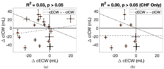
Figure 3. Changes in calf intracellular water (cICW) in ml versus changes in calf extracellular fluid (cECW) in ml. (a) contains data for all patients whereas (b) includes data for CHF patients only. The dotted line indicates a net zero change in cTW and the dashed line represents the linear best fit line. Patients with changes in calf volumes above the dotted line had net increases in cTW and patients with changes below the dotted line had net decreases in cTW.
Download figure:
Standard image High-resolution imageTable 2. Selected measured parameters at the beginning (Initial) and end (Final) of the hemodialysis session. All listed p-values are for paired t-tests. ns = not significant (p  0.05), * = p
  0.05. There were no statistically significant differences between CHF and non-CHF patients for any parameter at the start (Initial) or end (Final) of the hemodialysis session, nor were there statistically significant differences in the changes in these parameters (unpaired t-tests using Satterthwaite’s approximation).
| All patients | Non-CHF | CHF | |||||||
|---|---|---|---|---|---|---|---|---|---|
| Initial | Final | p | Initial | Final | p | Initial | Final | p | |
| cECW (ml) |  |
 |
* |  |
 |
ns |  |
 |
* |
| cICW (ml) |  |
 |
ns |  |
 |
ns |  |
 |
ns |
| cTW (ml) |  |
 |
ns |  |
 |
ns |  |
 |
* |
| cECW/cTW |  |
 |
ns |  |
 |
ns |  |
 |
ns |
CNR ( m m kg kg ) ) |
 |
 |
ns |  |
 |
ns |  |
 |
ns |
| Weight (kg) |  |
 |
ns |  |
 |
ns |  |
 |
* |
There were statistically significant correlations between changes in cTW (ml and %) and UFV as a percentage of initial weight for all patients ( and 0.27, respectively, both p-values
  0.05, full table of correlations can be found in table 3, see also figure 4). There was also a statistically significant, correlation between cTW (%) and UFR normalized by weight (R2 = 0.23, p
  0.05).

Figure 4. Percent changes in cTW versus UFV removed as percentage of initial weight. (a) contains data for all patients whereas (b) includes data for CHF patients only.
Download figure:
Standard image High-resolution imageTable 3. Correlations between changes in calf volumes and selected measured parameters. Listed values include an  value with p-value in parentheses. ns = not significant (p
  0.05), * = p
  0.05.
0.05.  = Dialysate sodium–serum sodium before hemodialysis. The threshold for High CNR was 0.1017
  m
m kg
kg .
.
Initial CNR ( m m kg kg ) ) |
UFV (%) | UFR (ml/h/kg) |  |
|||||||||
|---|---|---|---|---|---|---|---|---|---|---|---|---|
| All | High CNR | CHF only | All | High CNR | CHF only | All | High CNR | CHF only | All | High CNR | CHF only | |
 cECW (ml) cECW (ml) |
0.12 (ns) | 0.34 (ns) | 0.30 (ns) | 0.09 (ns) | 0.49 (*) | 0.33 (ns) | 0.08 (ns) | 0.50 (*) | 0.46 (*) | 0.05 (ns) | 0.00 (ns) | 0.00 (ns) |
 cECW (%) cECW (%) |
0.21 (ns) | 0.29 (ns) | 0.36 (ns) | 0.17 (ns) | 0.46 (*) | 0.30 (ns) | 0.15 (ns) | 0.44 (*) | 0.40 (ns) | 0.01 (ns) | 0.00 (ns) | 0.00 (ns) |
 cICW (ml) cICW (ml) |
0.02 (ns) | 0.09 (ns) | 0.24 (ns) | 0.18 (ns) | 0.37 (ns) | 0.29 (ns) | 0.14 (ns) | 0.41 (*) | 0.29 (ns) | 0.02 (ns) | 0.11 (ns) | 0.05 (ns) |
 cICW (%) cICW (%) |
0.02 (ns) | 0.08 (ns) | 0.48 (*) | 0.09 (ns) | 0.36 (ns) | 0.07 (ns) | 0.07 (ns) | 0.42 (*) | 0.08 (ns) | 0.00 (ns) | 0.11 (ns) | 0.02 (ns) |
 cTW (ml) cTW (ml) |
0.00 (ns) | 0.18 (ns) | 0.07 (ns) | 0.23 (*) | 0.52 (*) | 0.50 (*) | 0.19 (ns) | 0.56 (*) | 0.55 (*) | 0.00 (ns) | 0.08 (ns) | 0.04 (ns) |
 cTW (%) cTW (%) |
0.00 (ns) | 0.18 (ns) | 0.03 (ns) | 0.27 (*) | 0.52 (*) | 0.46 (*) | 0.23 (*) | 0.56 (*) | 0.52 (*) | 0.02 (ns) | 0.13 (ns) | 0.09 (ns) |
When considering only those patients with CNR  0.1017
  m
m kg
kg 3, there were statistically significant correlations between each of the calf volume changes and UFR and UFV (except cICW changes for UFV).
When considering only those patients with CHF, there were statistically significant correlations between cTW (ml and %) and UFV and UFR ( , all ps
  0.05). There was also a statistically significant correlation between changes in cECW (ml) and UFR normalized by weight (
 , p
, p  0.05).
There were no statistically significant correlations between the sodium gradient (dialysate sodium–serum sodium) and any volume change, and the only statistically significant relationship between Initial CNR and volume changes was for cICW (%) for only CHF patients ( , p
, p  0.05). There were also no statistically significant correlations between the study session duration and any calf volume changes.
3.3. Comparison of calf normalized resistivity to other metrics of fluid status
There were significant correlations between Initial CNR and Initial cECW/cTW ( , p
, p  0.001, see figure 5), and Initial CNR and pedal edema score (
 , p
, p  0.001, see figure 6). These correlations were approximately equivalent when considering only CHF patients (
 , p
, p  0.01 and
  , p
, p  0.05, respectively). There was no statistically significant correlation between Initial CNR and clinically determined fluid overload.
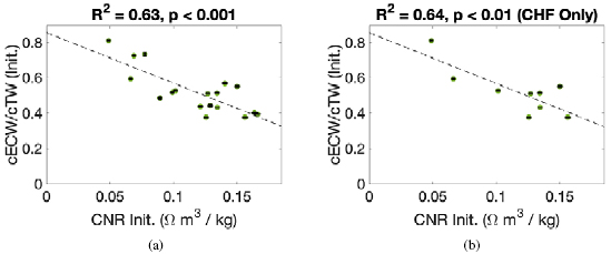
Figure 5. The initial cECW/cTW ratio versus the initial calf normalized resistivity (CNR). (a) contains data for all patients whereas (b) includes data for CHF patients only.
Download figure:
Standard image High-resolution image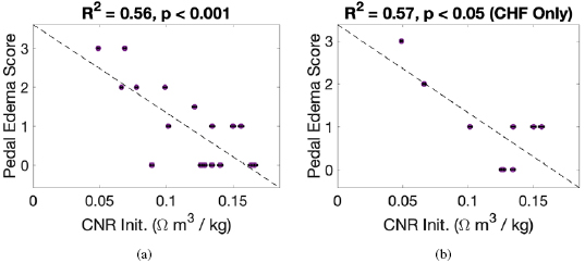
Figure 6. Pedal edema score (rated on a scale of 0–3, see section 2.5) compared with calf normalized resistivity (CNR). (a) Contains data for all patients whereas (b) includes data for CHF patients only.
Download figure:
Standard image High-resolution image4. Discussion
We found heterogeneity in the changes in calf volumes over the course of the hemodialysis session. Heterogeneity was particularly pronounced for patients with lower CNR (i.e. higher calf fluid overload).
4.1. Changes in cECW
Previous research has suggested that the calf is the last place to ‘dry out’ over the course of hemodialysis (Zhu et al 2008b). This means that depending on how close a patient is to their estimated dry weight, the ratio between fluid in the measured portion of the calf compared with fluid elsewhere will change. Patients very close to dry weight would be expected to have most of their excess fluid located in the calf. If we consider the relationship between changes in cECW and CNR (see figure 7), we find that the largest decreases in cECW occur at higher CNR, but not the highest measured CNR of all patients. We hypothesize that these patients have the largest changes in cECW because (1) most of their excess fluid is located in the calf and (2) they have lower fluid overload, so there is less refill of cECW from cICW (Isogai et al 1983). Patients with the highest measured CNR may already have been very close to their dry weight.

Figure 7. Percent changes in calf extracellular water (cECW) versus the initial calf normalized resistivity (CNR). (a) contains data for all patients whereas (b) includes data for CHF patients only.
Download figure:
Standard image High-resolution imagePatients with lower CNR show more variance. Of the patients with CNR below 0.1017  m
m kg
kg , 4/7 (57%) had no statistically significant change in cECW, 2/7 (29%) patients had decreases in cECW and 1/7 patients (14%) had an increase in cECW (the only patient in the study to have an increase).
Previous research has raised concerns about the impact of posture on changes during hemodialysis (Montalibet et al 2016). When an individual moves from a sitting or standing position to a supine position, extracellular fluid shifts from the legs to the torso (Medrano et al 2010). These shifts can last for several hours in healthy volunteers. Because extracellular fluid (presumably) also leaves the calf during ultrafiltration (Zhu et al 2008b), when a patient undergoing hemodialysis is supine after standing or sitting, changes in calf extracellular volume due to posture and changes due to ultrafiltration will be in the same direction and therefore difficult to distinguish from one another.
In this study, patients were mostly bedridden, and the majority of the sessions were performed in the morning after the patients had been asleep all night. The patients remained in a semi-supine position (legs horizontal at the same level as their buttocks with torso slightly elevated by a hospital bed and resting on pillows) other than briefly when a standing weight was performed. Thus, it is hypothesized that postural shifts would play less of a role in these patients when compared with healthy participants or more ambulatory patients. Additionally, some patients with high calf fluid overload did not experience much change in cECW even in the semi-supine position. This lack of fluid recruitment could indicate that posture is not playing much of a role for these patients; however, it could also mean these patients had impaired vascular refilling. Future work should consider the influence of posture and/or impaired vascular refilling on changes in calf fluid volumes during hemodialysis.
4.2. Changes in cICW
Changes in ICW during hemodialysis depend on a number of factors including (1) the plasma refill rate, (2) the ultrafiltration rate, (3) and dialysate concentrations. (1) The plasma refill rate is higher in patients with higher fluid overload (Machek et al 2010). Refill of the intravascular space from the interstitial fluid can cause a transient change in the osmotic pressure of the interstitial fluid, resulting in temporary fluid shifts out of ICW. (2) Low ultrafiltration rates can cause transient fluid shifts into ICW due to urea gradients that build up during hemodialysis (Pastan and Colton 1989, Akcahuseyin et al 2000). Simulations performed by Akcahuseyin et al suggest that these fluid shifts into ICW may also be more pronounced in low perfusion areas like the legs (Akcahuseyin et al 2000). (3) Dialysate concentrations cause changes in osmotic pressure in ECW that can cause lasting changes in ICW (Baigent et al 2001).
When considering all patients, there was no correlation between changes in cICW and CNR, UFV, UFR, or the dialysate serum sodium gradient. However, when eliminating the low CNR patients, there was a significant correlation between changes in cICW and UFR. Patients with normalized UFR values lower than 7.6 ml/h/kg all had increases in cICW and patients with normalized UFR values higher than 7.6 ml/h/kg all had decreases in cICW (see figure 8).

Figure 8. Percent changes in calf intracellular water (cICW) versus the average UFR normalized by patient weight for patients with CNR  0.1017
  m
m kg
kg . (a) contains data for all patients whereas (b) includes data for CHF patients only.
Download figure:
Standard image High-resolution imageBecause UFR was determined based on the target UFV in this study, the two are highly correlated ( , p
, p  0.001). It is expected that the correlation between changes in cICW and UFV are due to the correlation with UFR rather than an independent association. Additionally, the changes in cICW observed are likely transient and would not necessarily persist at equilibrium.
4.3. Changes in cTW
Five patients (30%) had increases in cTW over the course of the hemodialysis session. Four of these patients had decreases in cECW, but increases in cICW that exceeded the decrease in cECW. One patient had an increase in cECW and no change in cICW. Shifts into cICW can occur due to a variety of factors as described in section 4.2 and these patients did have relatively low UFR that could lead to fluid shifts into cICW. In order for cTW to increase, these patients must have had some shift of fluid into cECW from elsewhere in the body to make up for the fluid shifts from cECW to cICW. This could occur due to posture or possibly due to relaxation of the vasculature, which can occur during hemodialysis (Koomans et al 1984).
4.4. Heterogeneity for patients with low CNR
There was considerable heterogeneity among patients with CNR  0.1017
  m
m kg
kg (
( ). Of the seven patients, there were four different presentations with small
  for each. Because all these patients had high fluid overload, the relationship between fluid in the calf and the rest of the body may be different than for the patients that were closer to their dry weight. Indeed, the patients closer to dry weight more closely mimic the findings of those presented elsewhere (Zhu et al 2008a, 2008b, 2011 and Montgomery et al 2013), whereas the patients with low CNR seem to be divergent.
4.5. Comparison of fluid status metrics
CNR correlated with the cECW/cTW ratio at the start of the hemodialysis session and the pedal edema score, but not the clinically determined FO. Other researchers have observed a small but statistically significant correlation between CNR and a gold standard hydration marker (total extracellular volume as determined by bromide dilution divided by the total fat free mass measured by MRI) (Zhu and Levin 2015). The whole body fluid overload metric used here was calculated from estimated dry weight and had a number of participants with negative fluid overload. This is not possible assuming the definition that the patient dry weight is the point at which a patient begin to experience hypotension during hemodialysis (Charra 2007). Additionally, estimated dry weight was not available for 3/17 patients. Future research should use a different whole body overload metric, for example whole body bioimpedance measurements or dilution measurements, to track the relationship between changes in whole body fluid compartments and calf fluid compartments.
4.6. Differences between patients with and without CHF
While patients with CHF did have statistically significant changes in cECW, cTW and weight and patients without CHF did not, there were no statistically significant differences between patients with and without CHF in terms of demographics or in terms of changes in calf volumes (see tables 1 and 2). Patients with CHF did have fewer patients with low CNR compared with patients without CHF (3/9 (33%) in the CHF group versus 4/8 (50%) in the non-CHF group). However, they differ by only one patient and this difference could be negligible in a study including additional patients.
4.7. Accuracy of calf volume estimations
Estimation of the total calf volume depends on the measured bioimpedance parameters  and
and  and calf circumference, along with parameters that are assumed constant over the course of the hemodialysis session (
 and
and  ). The mean fractional error (
 ) was 0.28% for
  and was 0.66% for
  . The calf circumference measurements (with 0.65% at the beginning and 0.87% at the end) therefore dominated cECW measurements (see equation (A.7)). Error in cTW and cICW was dominated by errors in
  (see equations (A.8) and (A.9)). Bioimpedance fractional errors were largest for patients with lower bioimpedance values.
Estimation of cICW and cTW depend on the high frequency resistance  . Although data in this study did not display the standard capacitive 'hook' effect (Scharfetter et al 1998), measurements were still impacted by high frequency artifacts from electrode mismatch (Bogónez-Franco et al 2009) and/or cable inductance (Freeborn et al 2018), and hence a cut-off frequency of 200 kHz was used to minimize the impact of these artifacts (see figure 9 for an example sweep with the artifacts and fits). Montalibet and McAdams have recently proposed a method for reducing the impact of electrode mismatch by performing an additional set of measurements with the leads reversed (Montalibet and McAdams 2018). Future work should evaluate this technique and other compensation mechanisms such as short/load calibration to ensure the accuracy of measurements with high frequency data.

Figure 9. Example of electrode mismatch 'hook' artifact at high frequencies (Bogónez-Franco et al 2009, Montalibet and McAdams 2018), along with two fits (one with a maximum frequency of 200 kHz (red) and the other with a maximum frequency of 1 MHz (yellow)).
Download figure:
Standard image High-resolution imageEstimations of all calf volumes depend on fluid resistivities  (all volumes) and
  (cICW and cTW) only. These values were assumed to be constant over the course of the hemodialysis session and also the same for all patients. If
  and
and  do not change significantly during hemodialysis, examining the percent change in calf volumes will cancel out the fluid resistivity terms, allowing ready comparison between patients. However, some changes in these fluid resistivities are expected during hemodialysis. If one assumes that the plasma sodium concentration equilibrates entirely with the dialysate sodium concentration, there could be variations in
  of at most 1% for patients with the largest gradients between the initial plasma sodium concentration and the dialysate sodium concentration. This would translate into a change in cECW due to changing
  of at most 0.67%; any changes larger than 0.67% would be due to other factors (i.e. volume changes). The intracellular resistivity
  is not expected to change much during hemodialysis as sodium and potassium concentrations inside cells are actively regulated.
4.8. Study limitations
This was a small, exploratory study with 17 patients. Future research should enroll additional subjects to further evaluate the presented findings. The present study involved measurements at the beginning and end of the hemodialysis session. Shifts in cICW that are presumed to be transient were observed; future research should repeat calf bioimpedance measurements several hours after hemodialysis to observe changes in calf volumes that persist at equilibrium. Future research should also investigate how factors that affect vascular refilling, such as posture and venous thrombosis, impact the present findings.
4.9. Translation to ambulatory CHF
The findings presented here suggest that changes in calf bioimpedance over the course of hemodialysis depend on a combination of the starting calf fluid overload, on the fluid removal rate, and on the total fluid removed. Patients with high calf fluid overload (as assessed by calf normalized resistivity less than 0.1017  m
m kg
kg ) had a heterogeneous and less predictable presentation than those with lower levels of calf fluid overload. In an eventual ambulatory setting, CHF patients would have the wearable bioimpedance monitor placed when a clinician assesses a patient to be at their 'dry weight' (i.e. little to no fluid overload). This means that patients should be at lower calf fluid overload levels, which had a clearer relationship with changes in calf fluid status compared with patients with higher levels of fluid overload. As a patient begins to retain fluid, the wearable monitor could alert the patient, caretakers, and/or clinicians accordingly and an appropriate intervention could be made, such as additional diuretics, an outpatient visit, or an earlier hospitalization. Providing this feedback loop for CHF patients will be a key aspect of managing CHF.
Fluid is removed about an order of magnitude faster during hemodialysis than in an ambulatory setting (0 to  1 l h
1 l h in hemodialysis versus 0 to
  1 l day
 in ambulatory CHF). This means that any transient fluid shifts that were documented during hemodialysis should not exist in an ambulatory CHF case and the body can be assumed to be at (ionic) equilibrium.
Another consideration in translation to an ambulatory CHF setting is the expected volume changes in that setting. In hemodialysis, a typical patient has up to 4 kg removed 3 days a week. In ambulatory CHF, patients are instructed to consult a physician when their weight increases by more than 2 kg over the course of a few days. Because these changes are on the same order, the calf bioimpedance system should be able to detect these changes so long as the device can consistently measure bioimpedance over a period of several days. However, the system would have to account for changes in posture affecting pooling of fluid in the leg.
Because patients in an ambulatory CHF setting will retain fluid relatively slowly, calf bioimpedance is expected to change much more slowly compared to the hemodialysis case. In order to maximize observed bioimpedance changes, we investigated ideal electrode placement for calf bioimpedance measurements in a study presented elsewhere (Delano and Sodini 2018). We found that percent changes in calf bioimpedance depend on where electrodes are placed on the calf and that the use of ring electrodes is most suitable to determine an average change in bioimpedance in the whole calf segment as point electrodes record bioimpedance that is dominated by the region near the electrodes.
5. Conclusion
Congestive heart failure (CHF) is a chronic medical condition characterized by fluid overload with high readmission rates. Here calf bioimpedance measurements were performed to begin to understand the relationship between changes in calf fluid status and the rest of the body. Calf bioimpedance measurements were performed before and after hemodialysis and different metrics of fluid status were measured. Changes in calf compartment volumes varied with calf fluid overload (as assessed by calf normalized resistivity) and ultrafiltration rate. There were larger changes in cECW among patients with lower calf fluid overload as the calf is the last place to dry out over the course of hemodialysis. Changes in cICW were highly variable for patients with high calf fluid overload than patients with low calf fluid overload. Among patients with low calf fluid overload, flow in and out of cells was governed by the ultrafiltration rate. In an ambulatory setting, patients will start 'dry' and ideally receive treatment before reaching the levels of fluid overload observed in some patients in this study. Translation of calf bioimpedance measurements to an ambulatory CHF setting may enable a feedback loop not currently available to patients, caretakers, and physicians that would help prevent fluid overload related hospitalizations.
Acknowledgments
The authors would like to thank Dr Maulik Majmudar, Dr Herbert Lin, Haley Dalzell, Bianca Lavelle, Divya Padmanabhan, and Rachel Lopdrup (all at Massachusetts General Hospital) for their assistance with clinical testing for this study. They would also like to thank Dr Thomas Heldt, Dr Collin Stultz, Jeff Ashe and Tom O'Dwyer for their insights, and Will Wang (Swarthmore College) for research assistance. Funding was provided by the MIT Medical Electronic Device Realization Center (MEDRC) and the MIT Center for Integrated Circuits and Systems (CICS).
Appendix. Estimating errors in calf volume measurements
Calf volume measurements cECW, cICW, cTW and CNR are measurements that involve multiple measurements with their own standard deviations. In order to calculate the standard deviation for cECW, cICW, cTW and CNR, the standard deviations for the variables  ,
,  and the circumference must be combined systematically. There are a number of rules that can be used together to calculate the overall standard deviation for a composite measurement that consists of multiple measurements with their own standard deviations (assuming the input variables are independent and fit a Gaussian distribution) (Taylor 1982). For each rule,
  is some combination of
  and
and  :
:


Consider, for example, cECW (see equation (9)). Assuming  and
and  are constant and therefore do not contribute to the overall standard deviation, there is a circumference term in the numerator, a resistance term in the denominator, and both are raised to the 2/3 power:

Using equations (A.3) and (A.5), the total error for cECW is

An analagous approach can be used to solve for the other measured quantities:


The factor used for  in equation (A.8) was calculated empirically.
The following equations were used to calculate the absolute or percent difference over the course of the hemodialysis session:


where the initial measurement is from before the hemodialysis session and the final measurement is from after the hemodialysis session.
To calculate whether two measurements were statistically significantly different, the t-statistic was calculated using the mean and standard deviation from both measurements and then the two-tailed p-value was calculated using MATLAB's tcdf function.
The standard deviations for  and
and  were calculated directed from the four measurements performed before and after the hemodialysis session. For the circumference measurements, repeat measurements were not available for all patients, so the mean fractional error
  calculated from patients with repeat measurements was used for all patients. The fractional errors were 0.65% before the session and 0.87% after the session.
Footnotes
- 3
The value of 0.1017
 m kg was selected because it is a threshold at which the largest difference between two patient CNRs occurs.


