Abstract
A new electromechanical finite element modelling of a vibration power harvester and its validation with experimental studies are presented in this paper. The new contributions for modelling the electromechanical finite element piezoelectric unimorph beam with tip mass offset under base excitation encompass five major solution techniques. These include the electromechanical discretization, kinematic equations, coupled field equations, Lagrangian electromechanical dynamic equations and orthonormalized global matrix and scalar forms of electromechanical finite element dynamic equations. Such techniques have not been rigorously modelled previously by other researchers. There are also benefits to presenting the numerical techniques proposed in this paper. First, the proposed numerical techniques can be used for applications in many different geometrical models, including micro-electro-mechanical system power harvesting devices. Second, applying tip mass offset located after the end of the piezoelectric beam length can result in a very practical design, which avoids direct contact with piezoelectric material because of its brittle nature. Since the surfaces of actual piezoelectric material are covered evenly with thin conducting electrodes for generating single voltage, we introduce the new electromechanical discretization, consisting of the mechanical and electrical discretized elements. Moreover, the reduced electromechanical finite element dynamic equations can be further formulated to obtain the series form of new multimode electromechanical frequency response functions of the displacement, velocity, voltage, current and power, including optimal power harvesting. The normalized numerical strain node and eigenmode shapes are also further formulated using numerical discretization. Finally, the parametric numerical case studies of the piezoelectric unimorph beam under a resistive shunt circuit show good agreement with the experimental studies.
Export citation and abstract BibTeX RIS
1. Introduction
Recently, piezoelectric power harvesting devices have shown their viability for converting mechanical energy into useful electrical energy that can be used to power remote, smart wireless sensor systems. Their applications include monitoring of intelligent infrastructure, aircraft and environmental monitoring systems and biosensors for the human body. As a profound alternative energy source, a few published literature reviews [1–7] have discussed how the piezoelectric vibration-based power harvester applications from macro-to-micro levels benefit researchers who are investigating further novel techniques. Designing self-charging and lifespan energy harvesting devices requires technical knowledge and understanding of mechanical and electrical tuning techniques, material or physical properties, mechanical energy sources, power conditioning electronic circuits, sensor systems, and miniature fabrication. However, before conducting a manufacturing process for these smart devices in such conditions, initial mathematical models using analytical and numerical techniques become an important tool for analyzing the electromechanical piezoelectric vibration power harvesting response behaviour. Consequently, the development of new concepts has attracted attention from some researchers. Starting with the simplified analytical lumped parameter models of piezoelectric structures [8–10], the electrical equivalent systems representing the electromechanical piezoelectric component and standard circuit interface were developed. Considering the required accuracy and the necessity of modelling the cantilevered piezoelectric power harvester with tip mass under base excitation, the development of analytical approaches using Rayleigh–Ritz methods were explored in an effort to analyze various parametric case studies for vibration power harvesters [11–13]. Kim et al [14] investigated the vibrational piezoelectric bimorph power harvester with the effects of tip mass offset using the Rayleigh–Ritz method. Their interest and focus were to model the system responses of short- and open-circuit resonance frequency with variable load resistances using tip mass configuration. Moreover, Erturk [15] further developed comprehensive analytical approaches using assumed-mode methods for Euler–Bernoulli, Rayleigh and Timoshenko piezoelectric beams with axial deformations. It was proved that by increasing a certain number of modes in the choice of admissible trial functions, the approximation solution converges to the analytical solution, especially for the fundamental resonance frequency response. Erturk and Inman [16] have focused on researching the closed-form distributed parameter system of the Euler–Bernoulli bimorph beam for investigating frequency response functions (FRFs) under variable load resistance. Wickenheiser and Garcia [17] further developed the analytical modelling of piezoelectric bimorph beams with magnetic tip mass located near the fixed ferromagnetic structures in order to magnify the driving frequency below the fundamental frequency of the system. Moreover, Lumentut and Howard [18–20] explored the development of the piezoelectric bimorph beam with tip mass under both multidirectional excitation and the strain field effects of the transverse and initial longitudinal forms, in an effort to investigate a broad range of case studies using mathematical investigations of the orthonormalized electromechanical weak-form technique and closed-form boundary value method. In scrutinizing the system response of the single piezoelectric beam in light of the existing literature, the typical optimal power output mostly depends on the first mode. For this case, Lumentut et al [21] investigated the strategy of increasing power output and widening the multifrequency band using the orthonormalized multielectromechanical dynamic equations reduced from closed-form boundary value methods. Various parametric case studies have been developed using new electromechanical multimode FRFs of multiple piezoelectric bimorph beams connected in series, parallel and mixed series–parallel connections.
Some finite element literature concerns the use of piezoelectric components as smart material systems and has shown a variety of engineering applications, the most notable of which have been devoted to ultrasonic transducers and active control systems, either with feedback gain control or sensing and actuation response systems. However, for the current research, these piezoelectric finite element models give the relevancy and basis that allow the development of new numerical techniques for modelling the electromechanical power harvester, as presented in this paper. In the ultrasonic transducer application, Allik and Hughes [22] and Allik et al [23] first introduced mathematical models of the linear constitutive equations of the three-dimensional (3D) finite element piezoelectric vibration model using variational methods. Later, comprehensive mechanical discretized elements for analyzing an ultrasonic piezoelectric rod resonator [24] and the phenomenological electro-acoustic modelling for ultrasonic probes [25] were developed. Further application of the piezoelectric finite element has been developed for the active dynamic control system using feedback gain control. Tzou and Tseng [26] developed the active dynamic control matrix equations of the distributed piezoelectric components onto plate structures using the Hamiltonian principle and the Guyan reduction technique. Other published research works that analyze the controlled transient response [27–29] and transfer function [30] behaviour have been further investigated using the negative velocity feedback control system. For sensing and actuation response systems, the actuation system response, using applied voltage into the piezoelectric actuator, activated the piezoelectric sensor to create voltage output and deformation of the laminated composite structures [31–33]. More recently, Thomas et al [34] formulated the shunted electrical circuit connected to the piezoelectric patches using the finite element control system of the beam structure. Since the actual piezoelectric components are covered with electrode layers, the piezoelectric finite element literature ignores the electrode effect by assuming that the electrical voltages for each element and node are independent. Only a few of the published papers related to control finite element modelling have taken the electrode effect into consideration by assuming equal voltage distribution on each piezoelectric element [29, 31, 34]. However, the previous works are only based on mechanical discretization, without considering the electrical elements that are discretized due to the effect of electrode layers. Ignoring the electrical discretized elements from the electrode layer can affect the electromechanical FRF of the piezoelectric power harvester using the closed-circuit system. Also, there are no other previous research works that investigate the electromechanical finite element frequency responses using the electromechanical discretized elements under base excitation.
In earlier studies of the electromechanical finite element response of piezoelectric power harvesting, Lumentut et al [35] initially developed an energy harvesting plate structure with the segmented piezoelectric element based on the Love–Kirchhoff plate theory for investigating frequency and transient response behaviour. However, at an earlier stage, this model only considers the voltage output from the piezoelectric element without including the electrode effect with complete derivation of the electromechanical discretization related to the system response. DeMarqui et al [36] further presented the cantilevered plate with distributed piezoelectric layers by including the electrode effect, as validated by Erturk and Inman [16] in the existing literature of the piezoelectric bimorph with tip mass. However, their proposed finite element model does not take into account the important physical issues of the electromechanical orthonormalized global matrix and scalar forms, and the mathematical techniques of electromechanical discretization. Aladwani et al [37] further investigated the dynamic magnifier using a spring system attached to the base structure of the cantilevered piezoelectric bimorph beam with tip mass. The system was used to model the optimized power harvesting frequency response behaviour. However, their proposed work neglects the electrode effect of the piezoelectric component for formulating the electromechanical discretized elements, and also ignores the offset effect of the tip mass measured between the tip mass centroid and the end of the bimorph. Further research investigating piezoelectric power harvesters has been conducted using solid finite element-based ANSYS multiphysics software. Zhu et al [38] investigated the prediction of power output of FRFs under the resistive shunt circuit. Moreover, Yang and Tang [39] developed the electrical equivalent circuit model using SPICE software, whose circuit parameters were adopted from the ANSYS simulation for predicting the power output. However, although ANSYS software provides capabilities of 3D, coupled field solid, and plane elements, it is not able to model the laminated beam elements. For the standard level of the energy harvesters, mesh generation using laminated beam elements is sufficient to model the laminated piezoelectric beam structures (e.g., unimorph, bimorph and multimorph).
In this paper, new numerical techniques of the electromechanical finite element vibration power harvester using the Euler–Bernoulli unimorph beam model are presented and validated with experimental studies. The numerical models proposed here provide new technical contributions for analyzing the interrelationship between coupled field equations, electromechanical discretization, kinematic motions, Lagrangian electromechanical dynamic equations and electromechanical finite element equations. These technical contributions provide clear insight into the new electromechanical finite element equations for power harvesting applications, which can be highlighted in the following points:
- In considering the effect of electrode layers, we introduce the new electromechanical discretization, consisting of mechanical and electrical discretized elements, to model the electromechanical finite element piezoelectric structure. The electromechanical discretized elements provide an important basis for formulating the FRFs using new electromechanical finite element dynamic equations.
- The elemental system dynamics of the piezoelectric unimorph beam, including tip mass offset, are reduced from the kinematic equations. It is found that the effect of the offset distance, measured from the tip mass centroid and the end of the unimorph beam, can result in extra terms in the mass matrix and the generalized input dynamic force vector. The benefit of applying the tip mass offset, located after the end of the piezoelectric length, is that it can provide a very practical MEMS power harvester design for any level of scalability. It can also avoid the use of material around the end of the piezoelectric length, which can readily be damaged because of its brittle nature.
- The established, new, electromechanical finite element approach can be used conveniently to model different levels of scalability, including the segmented piezoelectric element coupled with substructure and micro-electro-mechanical system (MEMS) devices.
- The proposed numerical techniques also provide a complement to study the laminated piezoelectric beam with electrode layers in different applications.
- Lagrangian electromechanical dynamic equations are developed to formulate the constitutive elemental matrices of the electromechanical finite element equations. The orthonormalized global matrices and global scalar forms can be further reduced to formulate new multimode electromechanical FRFs of the displacement, velocity, voltage, current and power harvesting, including the optimal power harvester. The normalized strain node and eigenmode shapes are formulated using discretized elements for convergence studies. Finally, the parametric case studies with resistive shunt circuits, based on the proposed novel electromechanical finite element and experimental validations, are also presented and discussed.
2. Coupled field equations of the piezoelectric energy harvester
Constitutive linear piezoelectric beam equations can be formulated using tensor electrical enthalpy concepts, which are based on the continuum thermodynamics that can be condensed using Voigt's notation and Einstein's summation convention [19, 40–42]. The electrical enthalpy of typical smart materials with lead zirconate titanate (PZT) can be formulated under adiabatic and isothermal processes as

Notations of the piezoelectric parameters used here are stated in accordance with IEEE standards [43]. Here, the parameters  ,
,  ,
,  ,
,  ,
,  and
and  represent the piezoelectric elastic stiffness at constant electric field, piezoelectric coefficient, permittivity under constant strain, electric field, stress and strain, respectively. The parameter
  or
or  is given where
  ,
,  is the permittivity at constant stress and
  is the elastic compliance at constant electric field. Moreover, the common piezoelectric constant produced from the manufacturing company is in the form
  , where this can be modified by multiplying the plane stress-based elastic stiffness at constant electric field to give
  . The electric displacement of the piezoelectric element,
  , can be obtained by differentiating equation (1) with respect to
E
3. This electric displacement of piezoelectricity can be formulated as
, can be obtained by differentiating equation (1) with respect to
E
3. This electric displacement of piezoelectricity can be formulated as

Note that for the purpose of convenience in the forthcoming notations, the superscripts 1 and 2 that are used in the parameters of stress, strain, elastic stiffness, density and cross sectional area refer to the substructure and piezoelectric layers, respectively. Since the piezoelectric unimorph consists of active and inactive layers, the plane stress field from the inactive or substructure layer can also be formulated as

The piezoelectric stress field can also be formulated by differentiating equation (1) with respect to S 1, to give

Note that alternative derivations of equations (2) and (4) can also be obtained by using the enthalpy equation of state in terms of continuum thermopiezoelectricity, Maxwell's relations and Legendre's transformation [41, 44].
3. Kinematic equations for elemental beam and arbitrary tip mass offset
In this section, the kinematic motions for a continuous geometrical beam, as shown in figure 1, are derived from the different configurations at a series of points, resulting in the deformations and velocity of the body. However, the kinematics for the tip mass offset, whose motions are solely affected by the tip of the beam's transverse rectilinear ![$[\dot{w}_{abs}^{tip}\left( L,t \right)]$](https://content.cld.iop.org/journals/0964-1726/23/9/095037/revision1/sms497584ieqn15.gif) and angular
and angular ![$[\dot{\theta }\left( L,t \right)]$](https://content.cld.iop.org/journals/0964-1726/23/9/095037/revision1/sms497584ieqn16.gif) velocities, is a rigid-body motion with different configurations that result in extra terms in the kinematic equations. In reviewing previous studies, the most recently published papers on MEMS power harvesters [45–50] included the tip mass offset without scrutinizing its effect on the kinematic equations. The effect of the offset distance between the tip mass centroid and the end of the beam can effectively contribute to the mass matrix and the generalized input dynamic forces, as shown in section 4.3. It is important to note that the aim of formulating the kinematic equations is to formulate the Lagrangian functional energy forms that consist of the kinetic, potential and electrical energies of the piezoelectric unimorph, with the tip mass as given in the forthcoming section.
velocities, is a rigid-body motion with different configurations that result in extra terms in the kinematic equations. In reviewing previous studies, the most recently published papers on MEMS power harvesters [45–50] included the tip mass offset without scrutinizing its effect on the kinematic equations. The effect of the offset distance between the tip mass centroid and the end of the beam can effectively contribute to the mass matrix and the generalized input dynamic forces, as shown in section 4.3. It is important to note that the aim of formulating the kinematic equations is to formulate the Lagrangian functional energy forms that consist of the kinetic, potential and electrical energies of the piezoelectric unimorph, with the tip mass as given in the forthcoming section.

Figure 1. Kinematic motions of the beam and arbitrary tip mass offset.
Download figure:
Standard image High-resolution imageIn figure 1, the undeformed beam under base vector  moves from the fixed reference frame of oXZ to the initial reference frame of
  . Since the base vector, as the input excitation, moves from point
  to
to  at the designated reference frame, the position of point
  also moves to point
  with the same magnitude. As a result, the base vector creates the relative transverse deformation,
  , measured from point
  moving to the final point,
  . The absolute displacement,
  , can also be obtained from the fixed reference frame of oXZ to the final position. Note that the difference between the absolute displacement and the base vector defines the relative deformation. Moreover, the beam also carries an arbitrary tip mass offset whose kinematic motions must be considered. The position vectors of the tip mass start at point d to the final differential element at point
  , where the resultant vectors at points
  can be defined. The point of attachment,
  (deformation point at the end of the beam), to the tip mass centroid at point
  can be viewed as the offset of the tip mass. The origin of tip mass centroid can be determined from the differential element, using the extra position vector from points
  to
to  . As mentioned previously, since the tip mass was assumed to be a rigid body, its relative motions depend on the tip of the beam's motion at point
  .
.
The position vector,  , for the elemental beam can be defined as

where the position vectors,  and
and  , can be written as
In simplification of the linear assumption, the small angle,  , can be obtained after applying Taylor's theorem to give
  and
and  . As the initial position vector of the elemental beam,
  , is defined, the position vector,
  , from equation (5) can be differentiated with respect to time, which gives
Note that the absolute velocity vectors for the elemental beam and tip mass can be written as

For the elemental tip mass, the position vector,  , can be formulated as

where each position vector can be formulated as
Again, the linear system for the small angle,  , can be made using Taylor's theorem to give
  and
and  . In this case, the velocity of the elemental tip mass can be obtained by differentiating equation (9) with respect to time, to yield
The position vector,  , can be specified as the relative displacement with respect to the moving base support from reference frame
  to
to  , as
, as
The elemental beam strain can be obtained by differentiating  with respect to x, giving the typical Euler–Bernoulli beam theory as

Since the piezoelectric unimorph beam is viewed as the asymmetric structure with different material properties and geometrical dimensions, the asymmetric neutral axis [51] must be determined as presented in appendix
4. Electromechanical finite element vibration modelling of the piezoelectric energy harvester
In common practice, the surfaces of actual or physical piezoelectric material currently on the market are covered evenly with thin conducting electrodes, resulting in single voltage output during dynamic motions. As shown in figure 2(a), we chose the physical structure of the unimorph beam with an arbitrary tip mass offset, which consists of a piezoelectric material with a conducting electrode layer and a substructure. However, in figure 2(b), the electromechanical discretization, consisting of mechanical and electrical discretized finite elements, is completely different from the physical structure. In this situation, the electromechanical finite element discretization of the piezoelectric structure should be analyzed using the generalized multi-output electrical current from each element connected with an electrical parallel connection. Since the polarization is proportional to the stress field and the stress field is also proportional to the strain field [40, 44, 52], the polarization, P , and electric field, E , directions are chosen in the three-direction (thickness) along the z-axis.
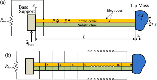
Figure 2. Electromechanical model of the unimorph beam with arbitrary tip mass offset under input base excitation, based on (a) a physical system connected electrically with the load resistance and (b) a new electromechanical finite element discretization.
Download figure:
Standard image High-resolution image4.1. Geometrical analysis of an electromechanical element
The first-order Hermite interpolation of the cubic displacement function is chosen here to formulate the unknown four degrees of freedom for the two-node unimorph beam element [53–55]. The cubic displacement function must satisfy the beam theory continuity conditions for the translation and rotational displacements for the general location of the elements. It is important to note here that the kinematic equations given in section 3 can be used to formulate the local element near the tip mass, as shown in figure 3, since the translation and angular velocities of the tip massʼs rigid body depend on the end of the unimorph beam of length, giving particular insight to formulating the complete electromechanical finite element equations.

Figure 3. First-order Hermite polynomials for a local unimorph element with an arbitrary tip mass at arbitrary nodes n−1 and n. Based on figure 2, by taking the example for n = 2.
Download figure:
Standard image High-resolution imageThe first-order Hermite interpolation in terms of the polynomial,  , and the unknown nodal displacement,
  , for the elemental beam can be formulated as

The property of Hermite polynomials for modelling the translation and rotation at the nodes can be formulated in terms of the l-derivatives to give
where xn
is the location at the nth node and  is the Kronecker delta with the property

Corresponding to equations (15) and (16), the lth derivatives of w(x, t) can be written as

or they can be formulated in terms of the unknown nodal displacement forms as

Note that equation (18) clearly shows certain physical meaning after applying equations (15) and (16), giving the nodal displacement forms as a function of time. Corresponding to index notation from equation (15), equation (14) can be modified by applying equation (18) to give

To find four terms of first-order Hermite polynomials, the property given from equation (15) can be used to identify four elemental boundary conditions for each degree of freedom at the nodes. In such conditions, the cubic equations with four unknown coefficients for each degree of freedom at the nodes can be used, and the results of the Hermite polynomials can be formulated after simplifying to give
Corresponding to equation (14), the simplified first-order Hermite interpolation function of the unimorph beam can be modified into a matrix form to give

where
Each parameter from equation (22) can be written in terms of the elemental displacement vector, u, and shape function,  , for each node as

Corresponding to equation (13), the strain–displacement relationship, in terms of the differential form of the shape function of the piezoelectric unimorph beam, can be formulated by substituting equation (21) to give

where the differential form of the shape function of the strain–displacement relationship can be formulated as
where
The elemental discretized electric field, E , induced by the strain field due to input ambient vibration, can create a polarization in the piezoelectric material in the z-direction along its thickness, generating the electrical voltages. The electrical field is a function of the electrical potential, with a negative gradient operator given by

where  is the electrical potential with linear assumption, the parameter
  is the shape function over the interval
  , and zn
indicates the distance from the asymmetric neutral axis, as given in appendix
, and zn
indicates the distance from the asymmetric neutral axis, as given in appendix  is a gradient operator for the first derivative of the shape function with respect to the thickness direction, giving
  . In this case, the discretized electric field can be reformulated as

The expression of the stress field in partial differential shape function form can be formulated for both piezoelectric and substructure elements by substituting equations (24) and (28) into equations (3) and (4), to give
The electric displacement vector of the piezoelectric component can be formulated by substituting equations (24) and (28) into equation (2) to give

4.2. Lagrangian electromechanical finite element equation
Constitutive electromechanical finite element dynamic equations are developed for modelling the elemental piezoelectric unimorph with the tip mass offset under input base transverse excitation. The functional energy forms using the extended Lagrangian formulation consist of kinetic (KE), potential (PE) and electrical (WE) energies, and nonconservative work (WF). The extended Lagrangian equation can be written as

where  ,
,  and
and  or
or  .
.
The kinetic energy can be formulated based on the mass density of the piezoelectric unimorph and the density of tip mass, as
The derivation of equation (32) can be seen in appendix
The electrical energy term for the piezoelectric layer can be reduced as

The nonconservative work on the system, due to the input base excitation and electrical charge output, can be written as
The reduced form of equation (35) due to the input base excitation can be found in appendix
Corresponding to equations (24) and (29), the extended potential energy form can be reduced as
The extended electrical energy expression can be reduced by substituting equations (28) and (30) into equation (34), as
The extended virtual work, in terms of the expression of nonconservative energy, can be formulated by substituting equation (21) into (35) to give
The expressions given from equations (36)–(39) can be substituted into equation (31) to give two electromechanical dynamic equations. After simplifying, the first electromechanical dynamic equation due to the transverse bending form can be expressed as
The second electromechanical dynamic equation due to the electrical form can be expressed as
Equation (41) can be modified by differentiating with respect to time, to give
4.3. Element matrices of electromechanical dynamic equations
Constitutive electromechanical nonhomogeneous differential dynamic equations, in terms of equations (40) and (42), can be arranged into matrix form by including Rayleigh damping to give
where
It is important to note here that equation (43) consists of mass, stiffness, electromechanical coupling and piezoelectric capacitance matrices and dynamic force vectors. These parameters are modelled at the local electromechanical element, which is located between the end of the unimorph beam length and the tip mass. The contribution of the offset tip mass can be seen in the mass matrices and dynamic force vectors, which most of the existing literature has ignored. As the unimorph-based Euler-Bernoulli beam assumption is considered, the first term from the mass matrix (rotary inertia of the unimorph) can be discarded due to the contribution of the Rayleigh beam assumption. Also, the contribution of input base excitation to the cantilever unimorph beam mathematically affects the distributed input dynamic forces into all the elements. Note that when other elements of the unimorph beam are considered in the numerical simulation, the parameter for the tip mass should be discarded from the mass matrices and input dynamic force vectors.
4.4. Normalized global element matrices of electromechanical dynamic equations
Constitutive electromechanical finite element dynamic equations in global matrix form reduced from the global transformation of local elements can be formulated as
Note that the script terms  and
and  showing at each parameter in equation (45) indicate the global matrices corresponding to global displacement vectors at nodes (nodal degrees of freedom) and global electrical voltage vectors at elements (electrical degrees of freedom), respectively. For assembling the global matrices, the connectivity matrices whose discretized elements share the same node should meet the requirements of compatibility. As the unimorph beam is a cantilevered structure under input base excitation, the fixed boundary condition at the base structure must be employed in the global matrices. For this case, the derivations for the normalized electromechanical dynamic equations and FRFs can be solved and given in the next stage. The use of the MATLAB computer program not only provides the best method for solving this case, but also gives an efficient computation technique.
The solution form of time-dependent displacement can be stated in terms of the normalized modal vector and the time-dependent displacement generalized coordinate as
where the normalized modal matrix can be formulated as,

It should be noted that parameters  and
and  represent a set of the normalized modal matrix and generalized eigenvector, respectively. To obtain the eigenvector and the eigenvalue solution, the undamped mechanical dynamic equation from the stiffness and mass matrices should be nonsingular, since the eigenvalue equation,
  , can be used to find the nontrivial eigenvector. Note that the normalized modal matrix is the matrix whose columns consist of the normalized eigenvectors [56]. The elemental strain field of the unimorph beam given in equation (24) can be formulated in terms of equations (24) and (46) to give
It should be noted that the elemental strain node parameter,  , based on the normalized eigenvector, can be determined at certain elements and nodes of the system over the interval,
  . Note that collective data points for strain nodes along the unimorph beam can only be identified for each discretized element using the differential strain–displacement function,
  , and elemental normalized eigenvector,
  . The normalized eigenvector at certain elements can only be determined by separating the cell vector array from the normalized modal matrix in terms of the elemental degree of freedom and the multimode system.
Equation (47) can be used to diagonalize the mass, stiffness and damping matrices to simplify the computation technique. Substituting equation (46) into equation (45) and premultiplying the result by  gives
gives
or simplifying equation (49) becomes
Parameter  from the first line of equation (50) indicates the nodal dynamic forces of the discretized unimorph harvester model due to the input base excitation. Other normalized parameters from equation (50) can be stated as
It should be noted that the first two lines of equation (51) represent the orthornormality property of mechanical dynamic equations, the results of which indicate diagonal matrices.
4.5. Normalized global scalar form of the electromechanical dynamic equations
In simplification, the normalized global element matrices of electromechanical transverse equations from equation (50) can be reduced into scalar forms in order to formulate the multimode frequency analysis of the distributed piezoelectric component, as shown in figure 2(a). The electromechanical equations consist of the coupled field normalized differential equations for each elemental global coordinate component. In this case, the first form of the discretized electromechanical piezoelectric dynamic equation can be formulated for the multidegree of freedom (multimode) system,  , in terms of the number of normalized piezoelectric elements,
  , as
, as
The second form of the discretized electromechanical piezoelectric dynamic equation can be formulated as
Note that since the piezoelectric surface with the electrode layers is distributed evenly on the substructure layer, the coupled equation for the global coordinate system should be based on the electromechanical discretization, as shown in figure 2(b). The internal parallel connection, in terms of the Kirchhoff's voltage law and Kirchhoff's current law, can be used to formulate the electrical discretized elements as
For voltage output, the external load resistance can be used as an external circuit to connect all electrical discretized piezoelectric elements in a parallel connection, as

Multimode FRFs of the distributed piezoelectric unimorph can be formulated in several ways. First, one can modify the first term of equation (53), which algebraically corresponds to the number of the normalized piezoelectric elements. Second, one can employ equations (54) and (55) in the equations obtained from the first step. Third, one can apply equation (54) in equation (52). Fourth, the results obtained from the second and third steps can be algebraically solved using Laplace transforms, giving the result in matrix form. The superposition of equations for voltage multimode FRFs can be formulated after simplifying, as
The multimode FRF of the electric current output related to the input base transverse acceleration can be stated as
The power harvesting multimode FRF, related to the input transverse acceleration, can be formulated as
To formulate the optimal multimode FRF of power harvesting, the reduced optimal load resistance needs to be formulated first. For this case, equation (58) can be differentiated with respect to load resistance, and the differentiable power function can be set to zero to give the optimal load resistance as

where

It should be noted that the optimal load resistance can be substituted back into equation (58) to give optimal power harvesting. Moreover, the multimode FRF representing the transverse displacement relative to the input transverse acceleration can be obtained as
Before equation (61) is modified into the transverse displacement FRF with respect to the input transverse acceleration at any position along the unimorph beam (x), the characteristic transverse motion of the unimorph beam can be reformulated in terms of the natural normal mode multiplied by the time-dependent transverse displacement, using equations (21) and (46) to give
Moreover, the characteristic motions for tip mass offset over the interval  can be formulated using the characteristic motions of the tip of the beam. As mentioned previously, note that since the tip mass offset is assumed to undergo rigid body motion, its motion depends solely upon the tip of the beam's transverse rectilinear and rotation or slope motions. To this point, the transverse displacement response of the tip mass offset can be formulated as
Corresponding to equations (61) and (62), the FRF that relates the multimode transverse displacement to the input base acceleration of the unimorph beam can be formulated as
For tip mass offset, the multimode transverse displacement FRFs can also be formulated in terms of equations (61) and (63) to give
For experimental study, a laser Doppler vibrometer was used to capture dynamic responses from the small beam and tip mass structures under input base motion, thus giving the absolute motion. For this case, equations (64) and (65) need to be modified in terms of the absolute motion. Since the combination of the base and relative motions defines the absolute motion, the multimode FRFs of absolute transverse displacement and velocity at any position along the unimorph beam and the tip mass offset can be formulated as
5. Experimental validation: results and discussion
In this section, the multimode FRFs for the velocity, electrical voltage, current and power outputs using the new electromechanical finite element equations are investigated and validated through experimental studies with variable load resistance (resistive shunt circuit). The input base transverse acceleration onto unimorph structures was chosen to be 1 m s−2. The piezoelectric unimorph structure was made from PZT PSI-5A4E material (Piezo Systems Inc., Woburn, MA), and the rigid body of the offset tip mass was subsequently attached. The geometrical structures of the piezoelectric unimorph with tip mass offset can be seen in figure 4, and details of the tip mass geometry, including formulas, can be seen in appendix

Figure 4. Geometry of unimorph beam with tip mass offset.
Download figure:
Standard image High-resolution imageTable 1. Properties of the piezoelectric unimorph system.
| Material properties | Piezoelectric | Brass |
|---|---|---|
Young's modulus,  (GPa) (GPa) |
66 | 105 |
Density,  (kg m−3) (kg m−3) |
7800 | 9000 |
| Piezoelectric constant, d31 (pm V−1) | −190 | — |
Permittivity,  (F m−1) (F m−1) |
1800 
|
— |
Permittivity of free space,  (pF m−1) (pF m−1) |
8.854 | — |
As shown in the experimental setup in figure 5, the cantilevered piezoelectric unimorph beam with the tip mass offset was clamped to the base structure under input dynamic excitation. The input acceleration from the base structure was measured using a B&K accelerometer. The B&K exciter connected to the power amplifier was used as the input dynamic excitation. The wave function generator connected to the power amplifier was used to control the input excitation using the sine sweep from the frequencies of 5 Hz to 1000 Hz, with frequency increments of 0.3125 Hz and 40 averages controlled from the B&K Fast Fourier Transform (FFT) Pulse analyzer software, in order to obtain a very smooth frequency response and to avoid aliasing components. Dynamic velocity of the tip mass offset was measured using a Polytec laser vibrometer with a measurement range full scale of 500 mm s−1 and a low pass filter setting of 22 kHz. Before operating the laser, a small reflecting film was attached to the top of the tip mass. Moreover, all signal measurements from the accelerometer, piezoelectric unimorph, and vibrometer were connected to the sophisticated B&K FFT Analyzer 3560B data acquisition device, which has five channels with a maximum frequency span up to 25.6 kHz. All processing signals through the analyzer displayed the measurement results using the FFT pulse software. Note that all sensitivities for scaling factors given from the B&K accelerometer of 9.633 mV m s−2, and from the laser vibrometer of 125 mm s−1 V (8 V m s−1), were inserted into the FFT pulse in order to obtain the correct results. Since the acceleration is given in per-unit acceleration in m s−2, all results of the FRFs given from the experiment and the numerical analysis in the next stage are given in per-unit acceleration in m s−2. Note that the B&K pulse software also provides the facility (a unit organizer) for modifying the units of amplitude of FRF; the amplitudes from the laser measurement can be stated in the velocity or displacement per-unit acceleration.
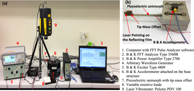
Figure 5. (a) Experimental setup and (b) piezoelectric unimorph beam with tip mass offset clamped on the base structure.
Download figure:
Standard image High-resolution imageThe first four modes of the unimorph beam, as shown in figure 6, can be used to identify the smoothness of mode shapes using the different sizes of a number of discretized elements. Although the resonant frequencies with discretization using a lower number of elements seem to be quite close to each other, the mode shapes seem to be quite coarse. These results show that the proposed 50 electromechanical discretized elements appear to be sufficient to provide accurate results that can give smooth mode shapes, including the natural frequencies. With the 50 electromechanical discretized elements, the strain node along the unimorph beam, as shown in figure 7, can be determined using the inflection point of the second order differential shape function of the strain–displacement relationship, as shown in equation (48). As the surfaces of the piezoelectric material are covered with the electrode layers, the inflection point can be used to identify the location of strain nodes along the beam, indicating the change of strains (tension and compressive strains) between two segments of the piezoelectric structure. This can avoid the reduction of the power output at the second or higher modes. Further details of the parametric strain node cases associated with the experimental study, in terms of electrical connection patterns, can be discussed in future investigations. Our main purpose in this numerical study is to present the new electromechanical finite element vibration techniques and show the validation with experimental studies.

Figure 6. Normalized displacement mode shape with (a) five elements, (b) 10 elements, (c) 30 elements and (d) 50 elements.
Download figure:
Standard image High-resolution image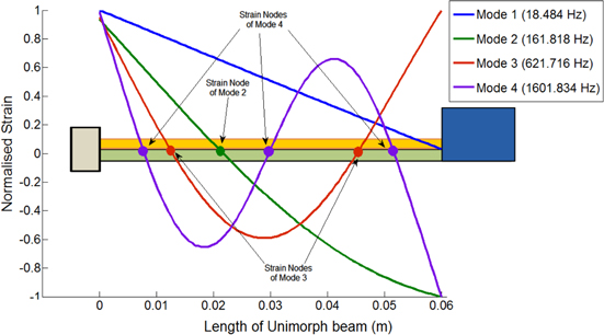
Figure 7. Normalized strain mode shape with 50 elements.
Download figure:
Standard image High-resolution imageIn figure 8(a), the absolute tip velocity FRFs and experimental results for the first mode show very good agreement under the variable load resistance. As we can see, higher amplitudes can be achieved when load resistances and frequencies shift from short circuits to open circuits. By viewing figure 8(b), the maximum tip absolute velocity responses at the short circuit and open circuit resonance frequencies of 18.5 Hz and 18.9 Hz were reached for load resistances approaching the lower and the higher values (from short circuits to open circuit load resistances), respectively. This behaviour can also be seen more obviously in figure 8(c). In many cases of vibration, the maximum dynamic displacement is generally avoided for most structures. It should be noted here that the power harvesting response can be shown to give the best results without having the maximum displacement, as we will discuss further in the next section. Note that the resonance frequency and amplitude response can shift due to resistive shunt damping from the variable load resistance, where this affects the electromechanical behaviour of the piezoelectric element. In addition, the physical behaviour of the piezoelectric unimorph, involving piezoelectric couplings and internal capacitance, also adds electromechanical damping and electromechanical stiffness. At this point, we realized that the damping effects consist of the mechanical and electrical components, due to the electromechanical behaviour of the dimensional structure, external load resistance and material properties of the piezoelectric structure and substructure. Identification of mechanical damping with very low load resistance can be obtained by matching the amplitude of the experimental and theoretical tip absolute velocity and voltage FRFs. The mechanical damping ratio of the first mode,  , under a very low load resistance of 562 Ω was obtained (approaching the short circuit resistance) because using the actual short circuit load resistance (Rload
= 0) will lead the theoretical voltage FRF to be zero, where the tip absolute displacement cannot be identified. This situation cannot be used to identify the voltage and displacement FRF behaviour of the electromechanical system.
, under a very low load resistance of 562 Ω was obtained (approaching the short circuit resistance) because using the actual short circuit load resistance (Rload
= 0) will lead the theoretical voltage FRF to be zero, where the tip absolute displacement cannot be identified. This situation cannot be used to identify the voltage and displacement FRF behaviour of the electromechanical system.

Figure 8. Tip absolute velocity FRF with (a) numerical (solid lines) and experimental results (round dots), (b) variable load resistances under the short circuit and open circuit resonance frequencies, and (c) 3D analysis.
Download figure:
Standard image High-resolution imageWith variation in the load resistance, the first mode of the voltage FRFs also varies while increasing load resistance, as shown in figure 9(a). In this case, the resonance frequency shifts to the higher value from short circuit to open circuit load resistances, followed by an increase in the amplitude. Note that when the voltage FRF with load resistance is close to open circuit, the amplitude remains constant.
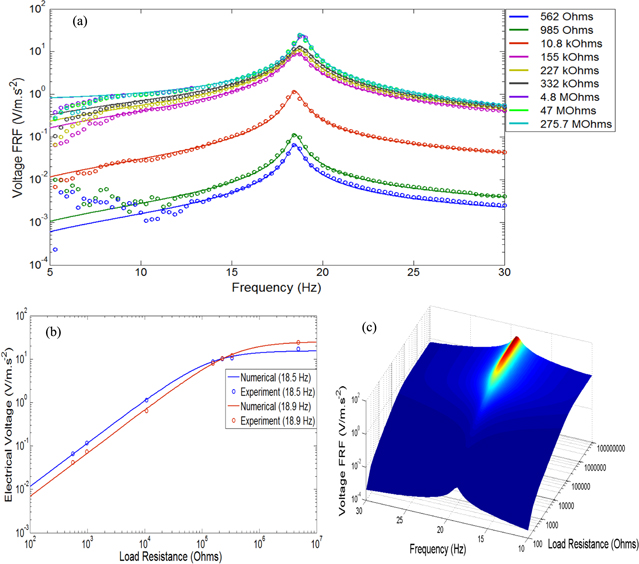
Figure 9. Voltage FRF with (a) numerical (solid lines) and experimental results (round dots), (b) variable load resistances under the short circuit and open circuit resonance frequencies and (c) 3D analysis.
Download figure:
Standard image High-resolution imageFigure 9(b) shows the trend of voltage behaviour under variable load resistance giving good agreement between numerical and experimental results. In general form, the voltage under short and open circuit resonances indicates a slight increase with increasing load resistance. However, the maximum open circuit resonance amplitude gives a higher value compared to the short circuit resonance when load resistance passes over the transitional or critical point of the short circuit and open circuit amplitudes. Note that the critical point of the amplitude response between short circuit and open circuit resonance frequencies shows the same amplitude. The change of frequency due to the variable load resistance can be seen more clearly in figure 9(c). For electrical current FRFs, as shown in figure 10(a), the trend shows the opposite behaviour of that of the voltage FRFs. The electrical current shows the highest amplitude when the load resistance approaches the open circuit. Again, in the opposite trend to the voltage response, the variation of electric current with variable load resistance under short circuit and open circuit resonance frequencies, as shown in figure 10(b), reaches the maximum amplitude with decreasing load resistance. This trend can be seen more obviously in the 3D current FRF shown in figure 10(c). Another important aspect related to the FRFs is the relationship between dynamic velocity, electrical voltage and current. The absolute velocity amplitude with the load resistance approaching the short circuit seems to increase, whereas the voltage amplitude decreases with increasing electrical current. Conversely, the velocity amplitude with the load resistance approaching open circuit tends to increase, whereas the voltage amplitude increases with decreasing electrical current.
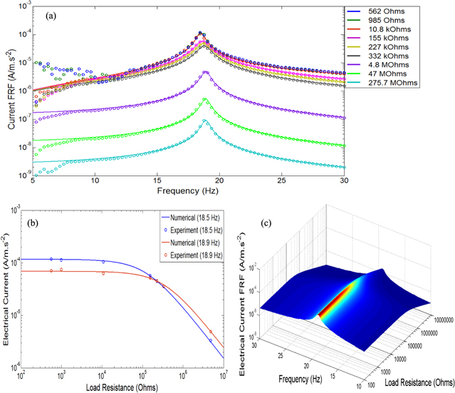
Figure 10. Electrical current FRF with (a) numerical (solid lines) and experimental results (round dots), (b) variable load resistances under the short circuit and open circuit resonance frequencies, and (c) 3D analysis.
Download figure:
Standard image High-resolution imageHowever, the power harvester FRFs, especially near the first mode response, as shown in figure 11(a), seem to behave with different trends where the short circuit and open circuit load resistances tend to decrease the amplitude. It can be said that the highest velocity amplitudes at the short circuit and open circuit load resistances do not show the highest power amplitudes. In different configurations with velocity, voltage and current, the variations in power harvesting under short circuit and open circuit resonance frequencies, as seen in figure 11(b), show two different optimum load resistances, giving the optimum amplitudes. In the 3D graph shown in figure 11(c), the optimum power harvesting amplitudes can also be seen clearly at the regions away from the short circuit and open circuit load resistances.
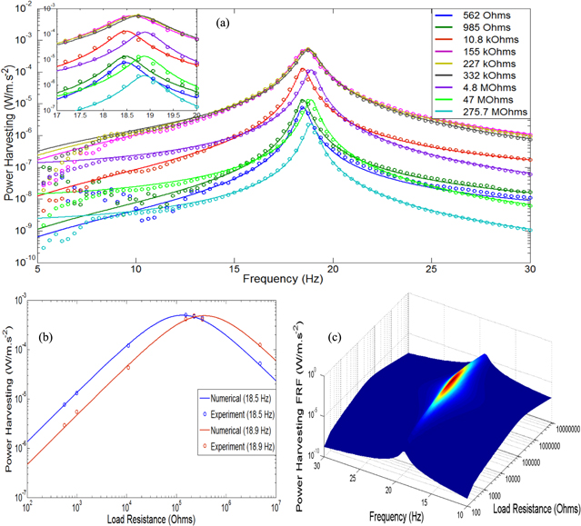
Figure 11. Power FRF with (a) numerical (solid lines) and experimental results (round dots), (b) variable load resistances under the short circuit and open circuit resonance frequencies and (c) 3D analysis.
Download figure:
Standard image High-resolution imageOptimal power harvesting, based on the optimal load resistance, can also be seen in figure 12(a), where the absolute maximum power amplitude point coincides with the load resistance of 227  at the resonance frequency of 18.70 Hz. However, the optimal load resistance in the off-resonance regions seem to approach and overlap with the load resistances of 155
  and 332
  , where the experimental results are also very close to the off-resonance regions, except for the driving frequency below 8 Hz due to unwanted noise. By scrutinizing the optimal power harvesting response, the numerical modelling result seen in figure 12(b) shows that ignoring the rotary inertia of the tip mass results in the shift of the resonance frequency to a higher value. The resonance difference is also more pronounced if the model ignores the offset distance of the tip mass measured from its centroid to the end of the unimorph beam length. Neglecting both the offset and rotary inertia of the tip mass results in a larger modelling error. It can be seen that when designing either a micro- or mesoscale power harvesting device, the mathematical model should include the effect of the offset and rotary inertia of the tip mass.
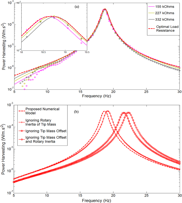
Figure 12. Identification of the optimal power FRF with (a) numerical (dashed lines) and experimental results (round dots), based on the optimal load resistance and related to other load resistances and (b) different cases of tip mass offset.
Download figure:
Standard image High-resolution image6. Conclusions
The new numerical study proposed in this paper addresses five important points.
- The electromechanical discretization was numerically developed, since the actual piezoelectric material covered by thin electrode layers only generates a single voltage across the electrical load. The electromechanical discretization introduced here consists of the mechanical discretized elements for elemental displacement fields and the parallel electrical discretized elements for multi-output electrical current. The previous published papers related to the piezoelectric finite element have not considered this in their mathematical modelling, although many of them showed different applications.
- Instead of developing the kinematic equations of the unimorph beam, the tip mass offset was formulated, since it contributes significantly to the mass matrices and the input dynamic force vector. The benefit of locating the tip mass with its centroid away from the end of the piezoelectric beam is that it allows for the modelling of various applications, especially MEMS power harvesters. The improved designs avoid contact between the brittle piezoelectric material and the tip mass. The previous published papers related to MEMS have ignored this in their mathematical modelling.
- The numerical techniques provide physical interrelationship between the electrode effect, coupled field equations, kinematic equations, electromechanical discretization and electromechanical dynamic equations.
- The reduced constitutive electromechanical finite element equations were further derived into global normalized scalar form of the electromechanical dynamic equations, in order to formulate the strain mode shape, eigenmode shape and multimode electromechanical FRFs. Unlike analytical techniques, the proposed new numerical solution techniques provided the benefit of analyzing the structure with different scalabilities, including MEMS devices.
- The comparisons between the numerical solution techniques and experimental studies have been discussed in terms of the variable load resistance, giving good agreement.
Overall, the experimental verification and parametric numerical case studies have been explored and have shown close agreement. For this paper, the proposed new electromechanical finite element modelling has proved that the velocity, current and power FRFs have shown very similar trends with the previous published analytical literature. These numerical results were also validated with experimental studies. Moreover, since the trend of optimal power harvesting FRF using different cases of the tip mass was presented, the new method showed that neglecting the rotary inertia of the tip mass resulted in a resonance frequency error. Notably, modelling errors occurred from ignoring the tip mass offset and ignoring both tip mass offset and rotary inertia. The other new aspect shown in using these numerical techniques is that the system models configured normalized strain node and eigenmode shapes using discretized elements for convergence studies. Further details of the frequency analysis using the strain node effect in terms of the electrical circuit connection patterns will be a focus of future studies.
The new numerical techniques can be a very useful tool for analyzing FRFs, displacement mode shape and strain node forms. These techniques can be applied to model different geometrical aspects for laminated structures and MEMS power harvester devices. In this case, since our main concern is presenting the new contribution of numerical techniques, it is important to validate the results obtained from numerical FRFs using experimental studies where the trends of the results were also shown to be very similar with facts established in previous analytical literature. Further applications for new aspects of power harvesting using the proposed numerical techniques can be demonstrated in future research studies.
Appendix A.: Determining the asymmetric neutral axis
In figure A1, the location of the asymmetric neutral axis, measured from the y-axis to the top surface of the piezoelectric layer, can be determined using the resultant force balance in the cross section of the unimorph structure to give

Figure A1. Cross-section of piezoelectric unimorph beam.
Download figure:
Standard image High-resolution imageManipulating equation (A1), the location of the asymmetric neutral axis can be reduced as

where coefficients  and
and  represent substructure elastic stiffness and piezoelectric elastic stiffness at a constant electric field, respectively.
Appendix B.: Determining the kinetic energy reduced from the kinematic equations
Corresponding to equations (7) and (11), the total kinetic energy of the system consisting of the elemental unimorph and tip mass offset, as shown in figure 3, can be formulated as

where
As mentioned previously, the translation and angular velocities of tip mass at the end of the unimorph beam length, L, as shown in figure 1, can be transformed into the local position of the end of the element,  , as shown in figure 3. The first part of equation (B.2) can be expanded as
Note that the first terms for each parenthesis from equation (B.3) must be zero, due to the Lagrangian functional form of the system only depending upon the relative translation and velocity of the unimorph, as expressed in section 4.2. The second terms for each parenthesis contribute to the input dynamic forces, and these terms can be moved into the nonconservative work section, as given in detail in appendix C. For the tip mass kinetic energy, the second part of equation (B.2) can be expanded as
Again, the first term of equation (B.4) must be zero. Moreover, the second to fifth terms must be zero because they contain the first mass moment of inertias for the tip mass body about the centroid at point g, as shown in figure 3, since the centroid of the tip mass is located on that centroid itself [57]. Again, the sixth and seventh terms can be moved into the nonconservative work section.
Equations (B.3) and (B.4) can simply be rewritten in matrix form as
The zeroth and second mass moment of inertias of the tip mass offset can be stated as
where  and definite integral forms of f(y, z) implied from equation (B.5) can be defined as
Note that equation (B.7) can be used for any operational integrations, not only in the kinetic energy derivation, but also for other Lagrangian energy forms given from equations (36)–(39).
Appendix C.: Determining the nonconservative work from the input base motion
As mentioned in appendix B, the contributions of nonconservative forces due to the input base excitation on the system were reduced from the kinetic energy. As a result, the virtual work done by nonconservative forces can simply be formulated in terms of their time-dependent response, using the Hamiltonian principle as

Note that from a mathematical standpoint, the functional form of Lagrangian's principle is reduced from the Hamiltonian principle using the variational method. Therefore, corresponding to equation (39), the virtual nonconservative works can be expanded by using the second terms for each parenthesis from equation (B.3) and the sixth and seventh terms from equation (B.4), as
Equation (C.2) needs to be further formulated by applying partial integration, and the result can be stated in the matrix form as
Appendix D.: Determining the geometry parameters of tip mass offset
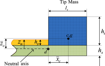
Corresponding to the parameters given by equation (B.6), the mass moment of inertias of the tip mass offset, as shown in figure 4, can be formulated. Note that as mentioned previously, the extra unimorph beam length, as shown in figure D1, also contributed to the tip mass offset. In this case, the zeroth mass moment of inertia can be stated as

and the second mass moment of inertia of tip mass offset at the point d, located at the end of the unimorph beam, can be reduced to give

where the offset distances measured from the tip mass centroid to the point d in the x- and z-axes can be formulated, respectively, as
Figure D1. Geometry of tip mass offset.
Download figure:
Standard image High-resolution image
Alternatively, and with the same result, the second mass moment of inertia of tip mass offset at the point d, located at the end of the unimorph beam, can straightforwardly be formulated as
