
Abstract
Liquid column dampers (LCDs) have long been used for the seismic vibration control of flexible structures. In contrast, tuning LCDs to short-period structures poses difficulty. Various modifications have been proposed on the original LCD configuration for improving its performance in relatively stiff structures. One such system, referred to as a compliant-LCD has been proposed recently by connecting the LCD to the structure with a spring. In this study, an improvement is attempted in compliant LCDs by replacing the linear spring with a spring made of shape memory alloy (SMA). Considering the dissipative, super-elastic, force-deformation hysteresis of SMA triggered by stress-induced micro-structural phase transition, the performance is expected to improve further. The optimum parameters for the SMA-compliant LCD are obtained through design optimization, which is based on a nonlinear random vibration response analysis via stochastic linearization of the force-deformation hysteresis of SMA and dissipation by liquid motion through an orifice. Substantially enhanced performance of the SMA–LCD over a conventional compliant LCD is demonstrated, the consistency of which is further verified under recorded ground motions. The robustness of the improved performance is also validated by parametric study concerning the anticipated variations in system parameters as well as variability in seismic loading.
Export citation and abstract BibTeX RIS
1. Introduction
With the advancement in high-strength materials and construction technologies, high-rise buildings are becoming an integral part of the modern urban infrastructure. These structures are relatively light, flexible and lightly damped and, therefore, the effects of vibrations caused by earthquakes and winds are more crucial. A conventional ductility-based design approach offers limited capacity of load resistance and energy dissipation under a more stringent definition of the design ground motions as well as the performance criteria. Over the last few decades, the use of technically feasible and economically viable control devices have emerged as a serious alternative for suppressing vibration effects on structures [1]. With smart structure technology, devices and systems are added to a structure to reduce the structural effects of vibration. Amongst several alternatives, the liquid column damper (LCD) was widely employed in the past for mitigating both wind- and earthquake-induced effects on structures. From its inception [2, 3] the LCD has attracted considerable attention from researchers in vibration control due to its reduced mass ratio requirement and consistent behaviour over a broader range of exciting frequencies. An LCD consists of a U-shaped liquid (water) tube supplemented with an orifice at the centre of the horizontal portion. In the course of motion, the liquid flows between the arms of the tube to actuate the control force. The control efficiency of the LCD is adjusted by tuning the vibration frequency of the liquid column to that of the main structure [3, 4]. In addition, the flow through an orifice helps in dissipating the input energy of the vibrations.
The applicability and effectiveness of LCDs [5, 6] to mitigate the effects of vibration on structures and their optimal performance is well established. The main advantage of an LCD over a tuned mass damper (TMD) is its lower mass ratio requirement [7, 8]. The LCD, being a long-period system, was primarily proposed to control the vibration of flexible structures with relatively longer periods. However, tuning the liquid column vibration to the vibration of short-period structures can be difficult. Due to a lack of tuning, the liquid column is not adequately mobilized in order to actuate the required control force or to dissipate the energy by flow through an orifice. However, the situation would be different in flexible (long-period) structures, for which the frequency of the liquid column in an LCD can easily be tuned to the vibration frequency of the structure, which will ensure enhanced vibration of the liquid column, leading to better control efficiency. The application of LCD for mitigating wind-induced vibration of flexible structures (e.g. tall buildings, towers, cable-stayed bridges, etc) is well developed and implemented in many important structures [9]. However, unlike wind-induced excitations, earthquake excitations contain high-frequency content (low period). Therefore, the short and stiff structures are quite vulnerable to earthquake ground motions. As it is difficult to tune the vibration of the liquid in an LCD to the frequency of short-period structures, several modifications have been proposed to the original LCD configuration. These modifications are designed to facilitate frequency tuning to short-period structures to help control earthquake-induced vibrations. In one such configuration, the LCD has been used as a TMD by connecting the liquid container to the main structure with a spring. This is referred to as a liquid column mass damper (LCMD) [10–12]. The superior efficiency of the LCMD over the LCD has been demonstrated for controlling narrow band excitations, such as those caused by wind [11, 12] as well as broad-band seismic excitations [13]. This system is also referred to as a compliant LCD [14, 15] because the compliant link between the LCD and the structure facilitates tuning. Earlier studies have proposed optimal design parameters for such systems based on the closed form expression suggested by Den Hartog [5]. This neglects the effects of structural damping and the relative motion of liquid in the container, which implies that the LCD is essentially acting as a TMD. The only design variables adopted are the ratio of the head-loss coefficient to the length of the liquid column in the tube [13]. More details of the design approach used in a damper system [16] and a comparison with other dampers [17] can be found elsewhere. Along with the lower value of mass ratios in LCDs, they also use water that is already used in the supply systems of the buildings, thus avoiding the addition of extra mass to the system. Furthermore, the displacement of the liquid column and the damper is much less compared to other damping systems, which offers more flexibility for satisfying the rattle space constraint, if present.
In the current study, an improvement is attempted in the compliant LCD by replacing the linear spring of the compliant LCD by a nonlinear flexible mechanism (spring) made of shape memory alloy (SMA) material. This device is referred to as an SMA–LCD in the following discussion. The hypothesis is that along with the required flexibility for frequency tuning, the SMA also dissipates energy by stress-induced micro-structural phase transition under cyclic loading to achieve improved control performance. The performance of the SMA–LCD system when subjected to earthquakes is assessed by a nonlinear random vibration analysis through statistical linearization of the phase-transitional force-deformation hysteresis of SMA and head-loss-induced dissipation caused by liquid flow through an orifice. The parametric study of stochastic response behaviour indicates the optimal design parameters for the SMA–LCD to ensure best performance. The optimal parameters are obtained through design optimization, and the respective performance is then compared with the conventional compliant LCD. The performance robustness of the optimal SMA–LCD system is further verified through time–history response analysis under recorded ground motions.
2. Response analysis of structure equipped with SMA–LCD
2.1. Equation of motion of structure with SMA–LCD system
The SMA–LCD system proposed in the current study for seismic vibration control of short-period structures is schematically shown in figure 1. The structure is modelled as a single-degree-of-freedom (SDOF) system. The SMA–LCD system is composed of an LCD attached to the main structure with a SMA spring. The equation of motion of the liquid in the tube can be written as [3, 8, 11]
where  is the density of the liquid,
  is the area of the tube,
  is the total length of the liquid in the column,
  is the length of the horizontal portion,
  is the length of the liquid column. The symbol
  is defined as the ratio of the length of the horizontal portion of the liquid tube to the total length of the liquid column, i.e.
  . The parameter
  represents the head-loss coefficient of the liquid as it flows through an orifice at the middle of the horizontal section of the tube. The displacement of the liquid column (i.e. change in elevation of the liquid column) is denoted by
  . The displacement of the liquid container relative to the SDOF system is denoted by
  and the displacement of the structure with respect to the ground is given by
  . The dot on any symbol represents its time derivative. The equation of motion for the liquid container can be written as
in which  is the mass of the container and
  is the restoring force developed in the spring attached between the liquid container and the structure. The restoring force developed in the spring is a nonlinear function of the relative displacement and velocity of the spring.
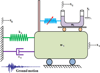
Figure 1. Schematic diagram of the SMA–LCD assisted SDOF system.
Download figure:
Standard image High-resolution imageAs the SMA–LCD is expected to substantially reduce the response of the structure, the behaviour of the structure can reasonably be assumed to be linear. A single degree of freedom system (SDOF) is considered to represent the structure. This is done to avoid the complexity of the structural model at the first instance of studying the performance of the SMA–LCD system when controlling the response of the structure. Further, Warburton and Ayorinde [18] and Ayorinde and Warburton [19] have demonstrated the possibility and accuracy of idealizing MDOF systems as an SDOF system by solving elastic structures, such as beams, plates and shells, while equipped with a TMD under the condition that their natural frequencies are well separated. It may also be mentioned here that TMDs or LCDs are conventionally designed to suppress the vibration of a single mode, preferably the fundamental mode of the structure. With these in view, the structure in the current study is adequately modelled as an SDOF system. The equation of motion of the SDOF structure can be written as
in which  and
and  are the mass, damping and stiffness of the SDOF structure to be controlled.
The equation of motion of the liquid column given by equation (1) contains a nonlinear term resulting from the dissipative flow through the orifice. This equation can be linearized by minimizing the mean square error among the actual nonlinear term and the linearized version of the same, i.e. ![$E\left( {{e}^{2}} \right)=E\left[ {{\left( 0.5\rho A{{\xi }_{l}}\left| {{{\dot{x}}}_{l}} \right|{{{\dot{x}}}_{l}}-2\rho A{{C}_{p}}{{{\dot{x}}}_{l}} \right)}^{2}} \right]$](https://content.cld.iop.org/journals/0964-1726/23/10/105009/revision1/sms499336ieqn16.gif) . This is known as stochastic linearization. The equivalent linear damping
. This is known as stochastic linearization. The equivalent linear damping  can be obtained in closed form as
  [20, 21], where
  is the root mean square (RMS) velocity of the liquid column in the tube. It is observed that the equivalent linear damping is a function of the response itself, i.e. the nonlinearity is still maintained in the linearized system. This requires an iterative algorithm for solving the resulting system of equations presented subsequently for the evaluation of responses.
2.2. Force-deformation behaviour of SMA spring and statistical linearization
The compliant device (spring) connecting the LCD to the structure is made of SMA. The restoring force developed in the SMA spring is denoted as  , which is a nonlinear function of the relative displacement and velocity of the container with respect to the structure. The force-deformation behaviour of the SMA spring is briefly illustrated in this section.
The SMA is available in several variants, such as nickel–titanium alloy, copper–zinc–aluminium alloy, copper–aluminium–beryllium alloy, etc The version of SMA that is referred to herein is the nickel–titanium alloy or Nitinol. The SMA can recover several percentage of strain after heating beyond a specific temperature, which is attained through micro-structural phase transition in the alloy. Another special property of interest for the application of SMA in LCD is its super-elastic force-deformation behaviour. This property is discussed in figure 2, which depicts the force-deformation behaviour. The SMA remains in an Austenite phase (OA) above a certain range of temperatures. The Austenite SMA starts transforming into Martensite (AB) when subjected to loading, resulting in a stress-plateau (AB). The force triggering the Austenite to Martensite phase transformation (A) is referred as the (forward)-transformation strength  , which is an important parameter governing the behaviour of the SMA-based system. The microstructural phase transition from the Austenite to Martensite phase is completed at point B. At a certain instant between the transition, the fraction of Martensite is denoted as
  . If loaded further, the transformed Martensite once offers further hardening (BC). When unloaded along the path CD, the Martensite SMA gradually recovers its deformation by backward transformation from the Martensite to Austenite (DE) phase, which is accompanied by a decreasing fraction of Martensite
  . The fully saturated or depleted state of Martensite phase is attained only after completion of phase transition, as indicated by points B and E. The interesting properties of such a flag-type hysteresis loop are that it is large enough to dissipate the input seismic energy and also leaves no residual displacement after unloading.
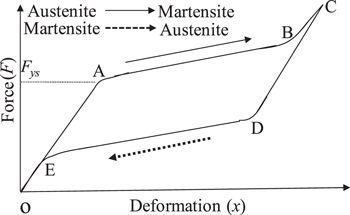
Figure2. Super-elastic load-deformation behaviour of SMA.
Download figure:
Standard image High-resolution imageSeveral phenomenological models are available to describe the hysteretic behaviour of SMA, out of which, the Graesser–Cozzarelli model [22, 23] has been proposed and employed to study the dynamic characteristics of many SMA-based systems. This model is a modification of the conventional Bouc–Wen model [24] of hysteresis with an extra term that takes care of the effect of super-elasticity. The parametric form of the model in a one-dimensional system is given as

in which  is the restoring force,
  is the relative displacement,
  is the initial stiffness of the SMA spring at the Austenite phase (OA) and
  is the transformation strength. The force for the transformation is very similar to the 'yield' force in the conventional elasto-plastic hysteresis. The parameter
  is a constant, determining the ratio of post- (AB) to pre- (OA) transformation stiffness similar to the ratio of the post- to pre-yield stiffness (rigidity ratio) in a bilinear system. The parameter
  controls the amount of recovery through backward transformation from Martensite to Austenite. The parameter
  controls the closeness of the forward and reverse transition to the idealized bilinear hysteresis. The parameter
  controls the slope of the unloading path (DE). The dot over a symbol implies differentiation with respect to time. The evolution equation for the back stress
  is governed by equation (4.2), and
  controls the type and size of hysteresis. In the special case
  , the Graesser–Cozzarelli model becomes identical to the Bouc–Wen model.
The nonlinear form (equations (4.1) and (4.2)) of the force-deformation equation are represented in an equivalent linearized form by a statistical linearization procedure. The restoring force developed in the super-elastic SMA spring is expressed as

in which  is the elastic part and
  is the hysteretic part of the displacement of the SMA. The procedure of statistical linearization is facilitated by simplifying the Graesser–Cozzarelli model by a simplified version [25] shown in figure 3 as
where  is the signum function defined as
in which a is the maximum displacement in the Austenite phase and b corresponds to the displacement triggering the Martensite transform. These parameters are determined from experiments. The statistically linearized form of the Yan and Nie model (equation (6)) is given as

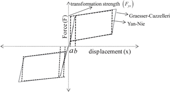
Figure 3. Simplified approximation of Graesser–Cozzarelli model.
Download figure:
Standard image High-resolution imageThe statistically linearized system properties are obtained by minimizing the least square error among the nonlinear terms of the model and its linearized version (equation (8)). The closed form expression for the linearized stiffness and damping is given as [19]


in which  and
and  are the RMS displacement and velocity of the container, respectively. Substituting for
  from equation (8) in (5), the restoring force in SMA is obtained as
where the statistically equivalent damping and stiffness are given by

With regard to the super-elastic behaviour of SMA, it must be pointed out that the property of super-elasticity can only be attained at specific range of temperature (0–40 °C) [23–25]. At temperatures much below 0 °C, the degeneration of the loop takes place to substantially affect its performance. With decreasing temperature, the stress level triggering the Austenite to Martensite phase transition decreases, leading to residual deformation after unloading. Furthermore, the Austenite to Martensite phase transition cannot be stress-induced [26] for temperatures much above 40 °C, which will also affect the super-elastic behaviour. Keeping in view that the mentioned temperature range falls within the range of ambient conditions, such dependence may not be a serious concern. It can be mentioned here that the desired temperature range for availing the super-elasticity can be altered by varying the composition of the alloys or by thermo-mechanical treatment, in which the effectiveness of the former is higher than the latter [26]. These techniques are adopted to tailor the properties of the SMA needed for specific applications, more details of which can be found from Ma et al [27].
A few limitations of the Graesser–Cozzarelli model of hysteresis for SMA are that it cannot represent the degeneration of the loop over a varying temperature range [23, 26]. In addition, it is observed that the strain rate and the number of loading cycles have minor effects on the hysteresis loop. Such dependence on the loading cycles, frequency and strain rate are reasonably assumed to be insignificant in the Graesser–Cozzarelli model. It may be mentioned herein that several improved versions of such models incorporating these aspects [26–28] can be considered in a future study.
2.3. Stochastic response of structure aided with SMA–LCD system
With the strength of stochastically linearized force-deformation equation of the SMA spring and the dissipation in the orifice, the equations of motion (1–3) can be rewritten as
The optimal performance of the system is ensured by properly tuning the frequency of its components to the frequency of the structure. For instance, the frequency of vibration of the liquid column  is tuned to the frequency of the structure
  in the case of TLCD. The tuning ratio for the TLCD in such a case is defined as
  . However, for compliant LCDs, the frequency of the liquid container
  is tuned to the frequency of the structure
  [13–15] and the tuning ratio is defined as
  in which the frequency of liquid container/tube
  is generally set to be equal the frequency of the liquid column
  .
.
The following notations are also introduced: the mass ratio of the liquid, i.e. the ratio of the mass of liquid to the mass of the structure  and the container mass ratio, which is the ratio of the mass of container to the mass of the liquid, i.e.
  . The frequency of vibration of the liquid column and the frequency of structure can be expressed, respectively, as
  , whereas the frequency of the container for the linear-compliant LCD is given by
  . For SMA–LCDs, this is defined in terms of the post-transformation stiffness of SMA as
  , in which
  is the post-transformation stiffness of the SMA spring, which provides the restoring force in the SMA–LCD. The transformation strength of the SMA spring
  is normalized with respect to the total weight of the liquid and the container as
  . These parameters can be substituted in Equations ((13.1)–(13.3)) for further simplification. The equations of motion (13.1, 13.2 and 13.3) for the SMA–LCD system, are combined as

where ![$\left[ M \right],\left[ C \right]$](https://content.cld.iop.org/journals/0964-1726/23/10/105009/revision1/sms499336ieqn57.gif) and
and ![$\left[ K \right]$](https://content.cld.iop.org/journals/0964-1726/23/10/105009/revision1/sms499336ieqn58.gif) are the combined mass, damping and stiffness matrix for the structure-SMA–LCD system. The displacement vector is given by
are the combined mass, damping and stiffness matrix for the structure-SMA–LCD system. The displacement vector is given by ![$\left\{ u \right\}={{\left[ \begin{array}{ccccccccccccccc} {{x}_{l}} & {{x}_{c}} & {{x}_{s}} \\ \end{array} \right]}^{T}}$](https://content.cld.iop.org/journals/0964-1726/23/10/105009/revision1/sms499336ieqn59.gif) and so is the vector of velocity
and so is the vector of velocity  and acceleration
  . The influence coefficient vector is given by
 ![$\left\{ r \right\}={{\left[ \begin{array}{ccccccccccccccc} 0 & 0 & 1 \\ \end{array} \right]}^{T}}$](https://content.cld.iop.org/journals/0964-1726/23/10/105009/revision1/sms499336ieqn62.gif) .The structure is assumed to be excited by a horizontal component of the Earthquake ground motion.
.The structure is assumed to be excited by a horizontal component of the Earthquake ground motion.
Dynamic-response analysis under seismic excitations generally employs a number of ground motions as input. This is in order to represent the wide variability in the ground motion characteristics commonly encountered in recorded motions. In stochastic analysis, such variability is represented through a stochastic model, which is conveniently expressed in terms of the power spectral density functions (PSDF) of the ground acceleration. One of the most commonly adopted models for seismic excitations is the Kanai–Tajimi model [29, 30]. This model treats the Earthquake as a stationary stochastic process, obtained by filtering white-noise excitations at the rock bed through a linear filter representing the ground. The filter equations are expressed as


in which  is the white noise intensity at the rock bed, characterized by its power spectral density
  . The parameter
  and
and  are the frequency and damping of the ground, respectively. The parameters
  ,
,  and
and  are the acceleration, velocity and displacement of the filter representing the ground. The respective PSDF function is expressed as
where  is the ordinate of the acceleration PSDF at frequency
  . The intensity of the white-noise excitations at the rock bed
  can be related to the RMS of the ground acceleration
  time history as [31]

Thus, the magnitude of the white-noise excitation  can be associated to the intensity of the Earthquake excitation. The Kanai–Tajimi excitation model is incorporated in the equations of motion by substituting equation (15.2) for equation (14). Thereafter, the equations (14) and (15.1) are rewritten together in state–space form as

where the state vector is defined as  . The matrix
 ![$\left[ A \right]$](https://content.cld.iop.org/journals/0964-1726/23/10/105009/revision1/sms499336ieqn76.gif) is the system property matrix and
is the system property matrix and ![$\left\{ w \right\}={{\left[ \begin{array}{ccccccccccccccc} \left\{ 0 \right\} & 0 & \left\{ 0 \right\} & -\ddot{w} \\ \end{array} \right]}^{T}}$](https://content.cld.iop.org/journals/0964-1726/23/10/105009/revision1/sms499336ieqn77.gif) is a vector of the white-noise excitations at the rock bed that characterizes the intensity of the ground motion. It can be shown that the covariance matrix of the response
is a vector of the white-noise excitations at the rock bed that characterizes the intensity of the ground motion. It can be shown that the covariance matrix of the response ![$\left[ {{C}_{YY}} \right]$](https://content.cld.iop.org/journals/0964-1726/23/10/105009/revision1/sms499336ieqn78.gif) can be obtained by solving an equation as [31]
can be obtained by solving an equation as [31]

The input matrix ![$\left[ {{S}_{ww}} \right]$](https://content.cld.iop.org/journals/0964-1726/23/10/105009/revision1/sms499336ieqn79.gif) contains zero terms except the last diagonal as
contains zero terms except the last diagonal as  . The matrix equation in (18) is solved to obtain the response covariance. For stationary excitations and responses, equation (17) reduces to a Lyapunov equation as

which may be solved by any standard Lyapunov solver. However, as the system properties are nonlinear, equation (19) requires number of iterations for convergence. The RMS value of responses are obtained from the covariance of the response as

The displacement of the main structure, container and the liquid column are the primary response quantities of interest.
The analysis presented herein for the evaluation of stochastic responses assumes that the excitation and responses are stationary stochastic processes. This can be extended to non-stationary earthquakes by adopting time-dependent characteristic frequencies and damping in the Earthquake ground-motion model.
3. Optimization of the SMA–LCD for best control efficiency
The response analysis shows that for compliant LCDs, the most important parameters to govern the behaviour of the controlled structure are the tuning ratio of the container  and the head-loss coefficient of the liquid
  in the column. The efficiency of vibration reduction is controlled by these two parameters [14, 15]. The vibration reduction is defined by the ratio of the system response and the response of the uncontrolled structure. Therefore, the RMS response of the controlled structure
  is normalized with respect to the response of the uncontrolled structure
  as
as

where  is the normalized response of the structure, representing the vibration-reduction efficiency. The parameters controlling the vibration-reduction efficiency are optimized to maximize the vibration-reduction capability. The relevant stochastic-structural-optimization (SSO) problem can be stated as

The frequency of liquid column  is assigned to be same as the frequency of vibration of the spring
  attached between the liquid container and the structure.
For the SMA–LCD, the respective design parameters can be identified as the tuning ratio, the head-loss coefficient and the normalized transformation strength of the SMA spring  . Following the adopted trend in the linear-compliant LCD, the vibration frequency of the liquid column is adjusted to be the same as the frequency of the container. The relevant optimization problem is then stated as

The optimization problems are solved using the nonlinear optimization routines provided in the MatLab Optimization Toolbox.
4. Response analysis under recorded ground motions
The consistency of the optimal response behaviour of the SMA–LCD as discussed in the previous section is verified further by evaluating its performance under recorded ground motions from real earthquakes. Therefore, a set of recorded ground accelerations are selected to evaluate the nonlinear time-history responses of the structure-LCD system with optimal LCD parameters. This involves integrating the dynamic equations of motions (equation (14)). The Newmark's beta scheme with average acceleration is used for integrating the equations of motion. This scheme efficiently incorporates the flag shape hysteresis of the SMA spring while evaluating its force-deformation characteristics. The adopted time steps are sufficiently small (0.0001 s) to ensure stability and accuracy of the numerical integration scheme. The time histories of the displacement of the structure, the displacement of the LCD and the displacement of the container/tube are obtained. These are then employed to validate the viability of the optimal response behaviour of the SMA–LCD as explored through SSO.
5. Numerical Study
5.1. Stochastic response analysis and optimization
The performance of the proposed SMA–LCD and its comparison to the compliant LCD is demonstrated through numerical simulation. The parameters adopted in the numerical simulation are listed in table 1. The displacement of the structure, liquid column and liquid container are the primary response quantities of interest. The variations of these responses are shown with respect to varying system parameters, such as the tuning in figures 4(a)–(c); the head-loss coefficient in figures 4(d)–(f); and the varying transformation strength of the SMA in figures 4(g)–(i). The trends of response behaviour for both types of compliant LCDs are similar. However, the control efficiency (displacement ratio) is remarkably enhanced by the SMA–LCD compared to the compliant LCD, which is also accompanied by the significantly reduced displacement of the liquid container as well as the displacement of the liquid column. It may be noted from these plots that the best control efficiency can be assured by not only adopting the optimal choice of tuning ratio and the head-loss coefficient only, rather, there exists an optimal value of the transformation strength of SMA for the same. The above discussion clearly indicates that the most important design variables are those that can be optimized in order to maximize the efficiency of the compliant LCD system. Therefore, parametric studies concerning the performance of both the systems and the optimal values of the respective design variables are obtained by optimization through numerical search techniques.
Table 1. Properties of the structure, LCD and compliant springs.
| Properties of the LCD | |||
|---|---|---|---|
| Properties of the structure | Linear LCD | SMA–LCD | Stochastic ground motion parameters |
| Time Period = 0.5 s Damping ratio = 2% | Mass ratio = 3% Tuning ratio = 0.95 Head-loss coefficient = 2.5 Density of liquid = 
|
Mass ratio = 3% Tuning ratio = 0.925 Head-loss coefficient = 3.0 Normalized SMA transformation strength = 0.05 Density of liquid = 1000 kg m−3 Hysteresis of SMA  = 0.10; = 0.10;  = 0.005 m = 0.005 m  = 0.07; = 0.07;  = 0.001; = 0.001;  = 2500; = 2500; 
|
 rad sec−1 rad sec−1  
|

Figure 4. RMS displacement of the (a) structure (b) the liquid column and (c) the container for varying frequency/tuning ratio. RMS displacement of the (d) structure (e) the liquid column and (f) the container for varying head-loss coefficient and RMS displacement of the (g) structure (h) the liquid column and (i) the container for varying transformation strength of SMA spring.
Download figure:
Standard image High-resolution imageAn important parameter that could affect the performance of a compliant LCD is its mass ratio. It may be recalled that the requirement of a relatively low value of mass ratio of an LCD versus that of a TMD is a remarkable feature of an LCD. Thus, it may be important to compare the performances between the two compliant LCD systems for varying mass ratios along with optimal choices for the other parameters. The optimal tuning ratios for varying mass ratios are shown in figure 5(a). It is observed that the optimal tuning ratio of the container for the SMA–LCD is much lower than that of the compliant LCD. A possible reason for this could be that the evaluation of the frequency of the SMA spring is based on post-transformation stiffness, which is much lower than the linear spring stiffness used for calculating the container frequency in the compliant LCD. The optimal head-loss coefficients, shown in figure 5(b) also indicate that the optimal head-loss coefficients for an SMA–LCD are much lower than those of the compliant LCD. This may be attributed to the input energy dissipation by phase-transformation-induced hysteresis in an SMA, which effectively reduces the share of the dissipation by the liquid flow through the orifice alone, as happens in a compliant LCD. The optimal transformation strength is shown in figure 5(c) for a given choice of the mass ratio. The important responses of the optimal systems are shown in figures 5(d)–(f). It is observed that the optimal performance of an SMA–LCD over the linear LCD is improved noticeably. The remarkably reduced liquid displacement is also an attractive feature of the SMA–LCD, as the requirement of large liquid displacement may not be accommodated in a practically feasible length of the liquid container/tube. In fact, in a few recent studies this aspect has been incorporated as a constraint in the process of optimization [32].

Figure 5. Optimal (a) tuning ratios (b) head-loss coefficient (c) transformation strength of SMA and respective (d) displacement ratio of structure (e) displacement of liquid column and (f) displacement of the container for varying mass ratios of the compliant LCDs.
Download figure:
Standard image High-resolution imageThe optimum performances of the compliant LCD systems are now studied for different levels of structural damping. The variations among the optimal parameters are shown in figures 6(a)–(c) and respective responses of the system are shown in figure 6(d)–(f). As stated earlier, the optimal SMA–LCD system has been proven more effective than the linear-compliant LCD. It is also observed that increasing the damping in the structure generally tends to reduce the efficiency of LCD systems. However, the relative performance improvement of an SMA–LCD over a linear LCD (figure 6(d)) is observed for the ranges of damping considered herein. It is also noted (figure 6(a)) that the tuning ratio decreases as the structure's damping increases. Previous studies on compliant LCDs assess the optimal frequency-tuning ratio by using the formulas given by Den Hartog [4, 11, 12] for a TMD. However, this is based on the assumption of zero damping in the structure. Moreover, the liquid in the container is also assumed to be in relative stagnation to allow for the LCD to act like a TMD, although the motion of the liquid in the container cannot be eliminated. In fact, the liquid motion is beneficial for the efficiency of the compliant LCD system. The trend shown in figure 6(a) indicates that structural damping may significantly affect the tuning ratio, and thereby the performance, of the LCD system.
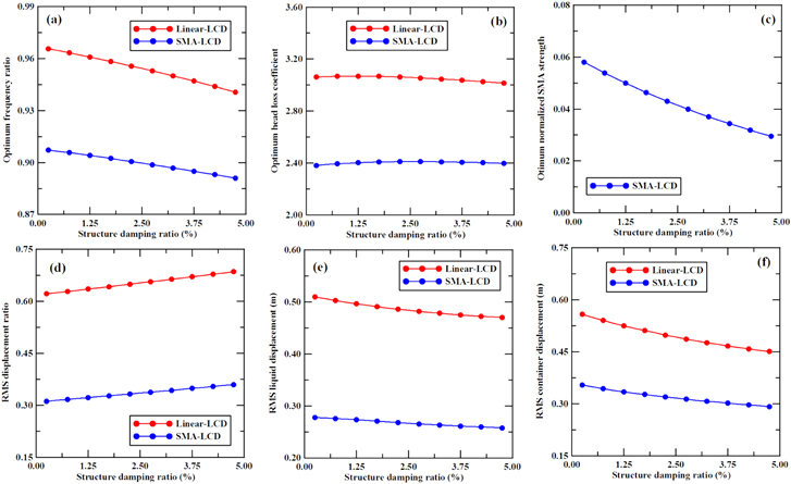
Figure 6. Optimal (a) tuning ratios (b) head-loss coefficient (c) transformation strength of SMA and respective (d) displacement ratio of structure (e) displacement of liquid column and (f) displacement of container for varying damping ratios of the structure.
Download figure:
Standard image High-resolution imageThe performance of the SMA–LCD has been studied for its varying dominant frequency content  caused by an earthquake as provided by the Kanai–Tajimi model. While plotting, the predominant frequency for the stochastic earthquake is normalized
  with respect to the frequency of the structure
  to be controlled. The dominant frequency content of the Earthquake
  is varied while keeping the structural frequency
  identical in order to study the effectiveness of the SMA–LCD under varying frequency content of the motion. The optimal parameter values are shown in figures 7(a)–(e) for the optimal tuning ratio, head-loss coefficient and transformation strength of the SMA spring, respectively. The optimal performances are shown in figures 7(d)–(f) for the displacement of the structure, liquid column and container, respectively. The improved performance of the SMA–LCD over the compliant LCD is obvious from these plots. It is observed that the efficiency of the compliant LCD sharply decreases under the resonating condition at which the dominant ground frequency matches the frequency of the structure. However, other than the resonating frequency, the improved efficiency of the SMA–LCD over the linear LCD is mostly insensitive to the variations of the ground-motion frequency. Therefore, the relative efficiency of the SMA–LCD over the linear LCD can be relied on a broad range of earthquake excitation frequencies and a single frequency optimization (preferably around frequency ratio 5) can be extended in such cases. Furthermore, the control efficiency is also observed to be mostly insensitive to such variations, except at resonating condition, which indicates robust performance.
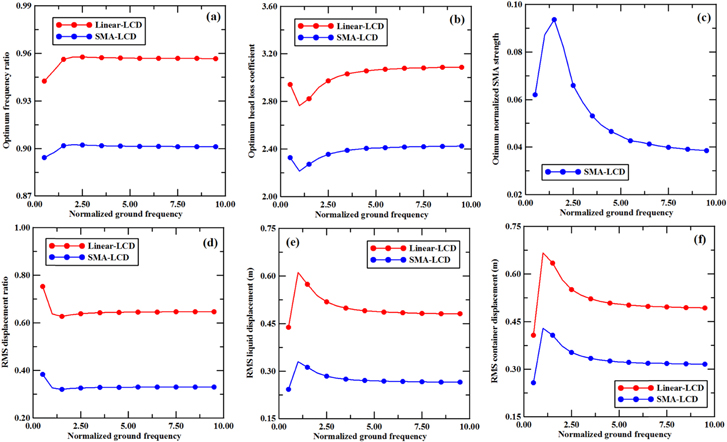
Figure 7. Optimal (a) tuning ratios (b) head-loss coefficient (c) transformation strength of SMA and respective (d) displacement ratio of the structure (e) displacement of the liquid column and (f) container for different dominant frequency content of the ground motion.
Download figure:
Standard image High-resolution imageIn the next section, the responses under different intensities of the Earthquake events (characterized by the magnitude of the white-noise excitation  at the rock bed) are furnished in table 2. These clearly indicate the significant improvement attained by the SMA–LCD over the conventional compliant LCD.
Table 2.
Optimal responses under varying seismic intensities  of earthquakes.
| Displacement ratio | Liquid displacement | Container displacement | |||||||
|---|---|---|---|---|---|---|---|---|---|
| Seismic intensity | Linear LCD | SMA LCD | increase (%) | Linear LCD | SMA LCD | decrease (%) | Linear LCD | SMA LCD | decrease (%) |
| 0.01 | 0.640 | 0.306 | 52.15 | 0.245 | 0.141 | 42.17 | 0.211 | 0.126 | 40.45 |
| 0.03 | 0.644 | 0.322 | 49.98 | 0.393 | 0.220 | 43.97 | 0.380 | 0.243 | 36.10 |
| 0.05 | 0.646 | 0.330 | 48.94 | 0.488 | 0.269 | 44.91 | 0.505 | 0.323 | 35.95 |
| 0.07 | 0.647 | 0.335 | 48.24 | 0.563 | 0.306 | 45.58 | 0.609 | 0.390 | 35.99 |
| 0.09 | 0.648 | 0.450 | 47.72 | 0.626 | 0.338 | 45.96 | 0.702 | 0.450 | 35.93 |
The response behaviour of the TLCD-assisted structure as presented in the previous section considers only the displacement response of the controlled structure, the displacement of the liquid column and the displacement of the liquid container. Although these are the primary responses of interest in a structure whose response is controlled by the damper, the acceleration of the main structure could also be an important quantity of interest. The reason for this is that the absolute acceleration represents the amount of force transferred to the structure and therefore governs the response of the secondary systems mounted on the structure. However, the addition of dampers in a structure does not significantly affect the acceleration response, as it does not significantly affect the overall stiffness. This is unlike the case of base isolation in which the acceleration to the structure decreases significantly because of the enhanced flexibility of the structure, which is caused by isolation.
5.2. Verification of optimal performance under recorded ground motions
The performance robustness of the optimal SMA–LCD system as obtained through stochastic analysis and optimization are subjected to deterministic time-history response analysis considering a suite of recorded ground motions. The selected earthquake records along with their dominant frequency content and peak ground accelerations (PGAs) are shown in table 3. As these parameters have an important effect on the structure's dynamic behaviour, the variability in their characteristics will be helpful in assessing the performance robustness of the optimal SMA–LCD system. These motions pertain to widely varying geological fault conditions and characteristics, as reflected in the salient characteristics shown in table 3.
Table 3. Set of ground-motion time histories selected for response evaluation.
| Serials | Earthquake | Year | Station | PGA (g) | Dominant Period (sec) |
|---|---|---|---|---|---|
| GM1 | Imperial Valley | 10/15/1979 | El Centro array5, 230 | 0.379 | 0.39 |
| GM2 | Kocaeli | 08/17/1999 | Yarimca 060 (Koeri) | 0.268 | 0.45, 0.54, 0.60 |
| GM3 | Loma Prieta | 10/18/1989 | LGPC, 000 | 0.563 | 0.47, 0.64, 0.70 |
| GM4 | Northridge Sylmar | 01/17/1994 | Sylmar-Converter | 0.897 | 0.59, 0.84 |
| GM5 | Superstition Hills | 11/24/1987 | PTS, 225 | 0.455 | 0.28, 0.64 |
| GM6 | Landers | 06/28/1992 | 24 Lucerne | 0.721 | 0.21 |
| GM7 | Duzce | 11/12/1999 | Duzce, 180 (ERD) | 0.348 | 0.41 |
The time histories of the important response quantities of the structure and of compliant linear and SMA–LCD systems are shown in figures 8(a)–(d) under the 1999 Kocaeli ground motions. Figure 8(a) clearly indicates that the proposed SMA–LCD improves the performance over the compliant LCD, along with a much-reduced level of liquid column displacement, as shown in figure 8(b). The lengthening of the period of vibration of the SMA–LCD compared to the compliant LCD is due to the reduced stiffness of the SMA spring in the post-transformation regime. The displacement of the liquid container is also observed (figure 8(c)) to be significantly reduced in the SMA–LCD. The comparison of force-displacement hysteresis of the vibration of the liquid column from both the LCDs also confirms this fact. It is also observed that the dissipated energies (head loss by the flow through the orifice) are mostly comparable. It is important to note from figure 8(d) that the damping force provided by the liquid sloshing in the SMA–LCD increases considerably from that found in the linear LCD, and with a much-reduced displacement of the liquid column. This might be due to the adaptive tuning of the higher-period liquid sloshing to the post-transformation vibration of the SMA spring, which is not possible to achieve in a linear spring. Further, the additional dissipation of energy through the hysteresis of an SMA spring (figure 8(e)) also contributes to the enhanced performance of the SMA–LCD over the compliant LCD.

Figure 8. Displacement of (a) structure (b) liquid column and (c) liquid container and associated force-deformation hysteresis of the (d) liquid column and (e) container restoring devices under 1999 Kocaeli earthquake.
Download figure:
Standard image High-resolution imageThe parametric studies consider the trend of response variations under varying mass ratios of the LCDs, as shown in figures 9(a)–(e). The response trends under the selected ground motions are shown in faint broken lines, while the mean trends are indicated by a thick solid line. The responses from the individual ground motions vary considerably owing to their varying characteristics, but the trends remain identical. The numerical values of the responses are not emphasized; rather, the trends of variations are compared to their stochastic counterparts (figures 5(d)–(f)). It is seen that the benefit of substantially reduced responses in the SMA–LCD over the compliant LCD is also available under recorded earthquakes.
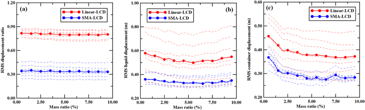
Figure 9. Parametric variations of RMS (a) displacement of structure (b) displacement of liquid column and (c) displacement of container in the optimal compliant LCD systems under varying mass ratio of liquid.
Download figure:
Standard image High-resolution imageThe response behaviour of the optimal LCD system under recorded motions is further studied under varying frequency content of the selected motions. For this study, the frequency content of the ground-motion records are adjusted by suitably varying the sampling intervals  of the individual motions. This is because the sampling interval determines the Nyquist frequency (
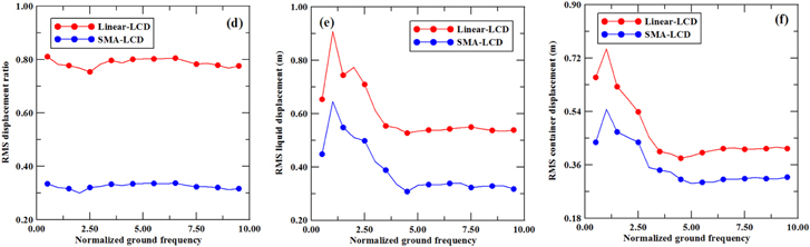
 Hz) and thereby the frequency content of a motion. A change in the sampling interval causes a linear shift in the frequency content. In fact, large variations are observed among the frequency content of the recorded ground motions, which could be very different from the idealized Kanai–Tajimi spectra. The power spectra of real earthquakes is not as smooth as the Kanai–Tajimi. The power ordinates and the predominant frequencies in real ground motions show erratic fluctuations. The variations among important response quantities of interest compared to the normalized predominant frequency of an earthquake are shown in figures 10(a)–(c). It is observed that the parametric trend of the stochastic analysis (figures 7(d)–(f)) matches agreeably well to the observed behaviour under recorded motions (figures 10(a)–(c)). The relative improvement of performance in the SMA–LCD over the compliant LCD is shown to be available under recorded ground motions having wide variations in their predominant frequencies and intensities.
Figure 10. The RMS (a) displacement of structure (b) displacement of liquid column and (c) displacement of container for the optimal LCD systems under different predominant frequencies from earthquakes.
Download figure:
Standard image High-resolution image
6. Conclusions
The performance of the compliant LCD is improved by the replacement of the compliant device (linear spring) with one made of a SMA material. The improved efficiency of the SMA–LCD system over the conventional compliant LCD is demonstrated by comparing the stochastic responses of both systems and by a comparison with the responses of the uncontrolled system subjected to random ground motion. The compliant LCD shows improved control efficiency compared to the usual LCD, which is further enhanced by the proposed SMA–LCD system. The displacement of the container and the liquid column in the SMA–LCD are much less than the compliant LCD. Parametric studies of stochastic responses reveal that apart from the tuning ratio and head-loss coefficient, there exists an optimum SMA strength that ensures the best control efficiency of the system. The improved performance of the SMA–LCD is further studied through time–history response analysis under recorded ground motions. The robustness of the improved control efficiency and associated response behaviour are also assessed under varying system parameters and intensities of earthquake loadings. Taken together, it is generally observed that the enhanced performance of the SMA–LCD over the compliant LCD can be relied on for controlling broad-band earthquake-induced vibrations in relatively short-period structures. However, the time-history study considering limited sets of ground motions is not exhaustive, and more sets of ground motions should be employed for comprehensive study of the robustness of the optimal performance of the LCD systems.
Acknowledgments
This research work was supported by the Fast Track Research Grant (Sr/FTP/ETA-35/2012) for young investigators provided by the Department of Science and Technology under the Ministry of Science and Technology, Government of India. This support is highly appreciated and acknowledged.