

Abstract
Power modulated microwave plasma jet operating in argon at atmospheric pressure was studied by spatio-temporally resolved optical emission spectroscopy (OES) in order to clarify the influence of modulation on plasma parameters. OES was carried out in OH, NH, N2 and  spectral regions using a spectrometer with intensified CCD detector synchronised with 101–103 Hz sine modulating signal. A special software, able to fit even the overlapping spectra, was developed to batch process the massive datasets produced by this spatio-temporal study. Results show that studied species with the exception of
  have balanced rotational and vibrational temperatures across the modulation frequencies. Significant influence of modulation can be clearly observed on temperature spatial gradients. Whereas for low modulation frequencies where the temperatures reach sharp maxima upon discharge tip, the high frequency modulation produces thermally homogeneous plasma.
Export citation and abstract BibTeX RIS
1. Introduction
The contribution of Czerny and Turner to the design of the mirror monochromators [1] enabled obtaining optical emission spectra with one-dimensional spatial resolution limited only by the imaging optics. Similarly, the introduction of intensified charge-coupled devices (ICCDs) [2, 3] enabled acquisition of images with very low exposure times, synchronised with eventual modulations of the investigated light source. Combining these two devices gave rise to a method known as phase-resolved optical emission spectroscopy (PROES) [4]. Generally, with standard devices and standard software tools, the data acquisition can be very efficient. Valuable results in this field have been reported for example in [5–10], where the authors investigated atomic lines taking advantage of the fact that in the spectrum, they appear separated from other emissions. The atomic lines can be used to provide information about the highly energetic electrons in the discharge.
The emission spectra can be also used to extract the temperature of the neutral gas [11], particularly molecular spectra at atmospheric pressure. The temperature can be extracted from the measured molecular spectra by fitting a simulated spectrum to the measured data, where the temperature is treated as a parameter of the fit, i.e. a Boltzmann distribution is assumed. Many groups have created their own software with this functionality [12–22]. Among the software packages for spectral simulation, particularly LIFBASE [23] and Specair [24] succeeded to gain popularity and are widely used.
However, none of the publicly accessible software packages provides the functionality of batch processing of large datasets containing overlapping molecular spectra which was necessary to obtain the spatio-temporal maps of rotational and vibrational temperature for the present work. We therefore developed a software, massiveOES, specifically to overcome these shortcomings which is freely available to the scientific community [25]. This paper, besides the plasma diagnostics results, also briefly discusses the data processing methods used by this software.
Atmospheric pressure plasmas are currently intensively studied due to their applicability in many technological fields such as material processing, waste treatment, spectrochemical analysis, surface treatment and biomedical applications. A deep knowledge of the fundamental processes governing these discharges and of the physical quantities necessary for a complete understanding of the plasma medium is thus of great importance for both basic and applied science.
Surface wave discharges (SWDs) are a class of discharges in which the plasma is sustained by high frequency electromagnetic waves propagating along the plasma boundary. SWDs have been widely studied empirically and theoretically and many applications are proposed [26, 27]. Previous experimental studies of surfatron discharges (as one of the SWDs) at atmospheric pressure adopted optical emission spectroscopy (OES) as the main diagnostic technique. The OES is one of the most widely used techniques as it is non-invasive, universal and experimentally relatively simple. It can provide good estimates of the electron concentration  , electron temperature
  and temperature of the neutral gas
  ; it also provides an estimate of the population of metastable states, and concentrations of some relevant species.
Surfatron discharges were investigated in pure argon [28–37], pure helium [38] and mixtures of Ar+H2 [34, 39], Ar+N2 [40], Ar+O2 [41], argon and water vapour [41], argon and methanol, ethanol, propanol and butanol [42] mostly as a function of the applied power and gas flow rate with microwave power continuously delivered.
It is expected that the microwave plasma excited using pulsed or modulated power would have a lower thermal loading of the substrate with higher density of active particles (such as electrons, ions, excited species, atoms, molecules, radicals, and so on) than the continuous wave plasma at the same mean power. The most common form of modulation is to use simple on/off variations; however, this puts high requirements on power amplitudes to overcome impedance difference as it is nearly impossible to match ignition phase and plasma operation simultaneously. Even with sufficiently strong power sources, this leads to a significant loss of power due to the reflection on imperfect matching. Thus a more advanced method is used to modulate the microwaves by an amplitude envelope. There were a number of surfatron discharges recently investigated in the power modulated regime using the sine wave envelope; these include pure argon [43–45], and mixtures of Ar+N2 [44], Ar+H2 [46], argon and tetrakis(trimethylsilyloxy)silane (TTMS) [47].
Recently, an observation of a transient vortex ring in the effluent of the power modulated surfatron discharge was reported [45]. The vortex seems to be responsible for previously observed shortening and widening of the visible discharge effluent [43] for a certain range of modulation frequencies. The investigated frequencies were chosen to represent the following three cases: (i) 90 Hz for the case when the vortex was not observed, (ii) 900 Hz for the case when the vortex was formed and (iii) 1710 Hz as the maximal frequency at which the used microwave generator was capable of following the modulations without significantly distorting the modulation envelope [45]. The vortex also significantly affects the mixing of the plasma activated argon with the surrounding atmosphere, thus also enhancing the plasma chemistry.
The current follow-up paper addresses the problem of heat transfer and energy exchange processes in the plasma effluent affected by the transient vortex. To achieve this, the measurements are resolved spectrally, temporally and axially at the same time.
2. Experimental
The spatially resolved and phase synchronised optical emission spectroscopy measurements were performed on plasma jet plumes using the set-up schematically visualised in figure 1.
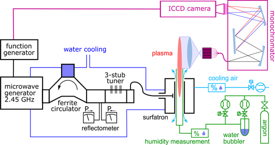
Figure 1. Schematic drawing of the experimental set-up.
Download figure:
Standard image High-resolution imageThe plasma was generated by a surfatron (SAIREM Surfatron 80)—particular type of surface wave driven plasma jet [48]. The microwave circuit feeding the surfatron consisted of 2.45 GHz generator (SAIREM GMP 20 KED), ferrite circulator, attenuator, 3-stub tuner and a coaxial cable. Some components of the microwave line (magnetron, circulator dummy load and surfatron body itself) were cooled by water. The generator worked in amplitude modulated (AM) mode with sine envelope of various frequencies (in this paper 90 Hz, 900 Hz and 1710 Hz were used) generated by function generator. The output power oscillated between 165 W in sine envelope minimum and 315 W in maximum. The reflected power was always kept below 3% at the mean power and below 10% at power maxima and minima. The actual microwave power envelopes can be seen in [45].
The plasma itself was ignited inside a fused silica discharge tube (2 mm inner diameter, 4 mm outer one) passing through the centre of surfatron body and sticking out 1 cm above the launching gap. Atmospheric pressure argon was used as a working gas and its flow rate was kept constant at 1 slm (standard litre per minute). To ensure reproducible humidity, water vapour was intentionally added to argon, resulting in a humidity constant of 2600 ppm(V). Vaisala DMT143 Dewpoint Transmitter was used for the humidity measurement. The accuracy in dew point measurement according to the manufacturer is ±2 °C, which corresponds to roughly ±400 ppm(V) for the absolute calibration. The relative changes are observable with higher precision. The plasma extended outside of the discharge tube and the effluent mixed with the surrounding atmosphere. Additionally, cooling air flowed around the discharge tube at the rate of 5 slm, and affected the plasma effluent as well. For more details on the three interacting gas environments please see [45].
A real image of the plasma effluent (13 mm above the discharge tube end) and a short portion of plasma inside the discharge tube (1 mm below the discharge tube end) was projected by a quartz converging lens (25.4 mm diameter, 200 mm focal length) to a vertical array of 64 optical fibres. The axially resolved optical emission signal was then introduced into the Jobin-Yvon HR-640 imaging monochromator (640 mm focal length, 1200 grooves/mm grating) and the resulting light pattern, corresponding to a desired portion of spectrum (attention was paid to four spectral regions, each 22 nm wide), was observed by an ICCD camera (Princeton Instruments PI-MAX2 1024RB-25-FG43, 16-bit greyscale resolution, 256 × 1024 pixels).
Recorded images were corrected by dark frame subtraction and by sensitivity normalisation for each spectral region. A deuterium lamp was used as a reference for sensitivity calibration of the whole system. The resulting image had a wavelength on the x-axis, axial position on the y-axis and shades of grey represented the spectral density. Each optical fibre in the array illuminated region of ≈3.5 pixel height. To obtain spatially resolved spectra, we performed a scalar product of each column of the image with a vector containing the Gaussian profile centred on respective fibre positions. Moreover, the ICCD camera was triggered by the same signal that was modulating the microwave generator. To achieve phase resolved scan over more than one full period, the set of 12 images was captured, with varying delay after the triggering signal, effectively scanning over the whole modulation period.
3. Data acquisition and data processing
Four spectral regions in near UV were observed, see figure 2:
- (i)306 to 328 nm where (v, v) bands of OH(A
 ) transition dominate. A trace of second positive system of N2(C ) emission, namely the bands, is also present between 310 and 316 nm and should be taken into account.
 - (ii)325 to 348 nm with dominant (v, v) bands of NH(A) emission overlapping with N2(C ) band at 337 nm. The (1,1) and (2,2) bands of N2(C ) are in the same spectral region but were not observable, despite the high vibrational temperature, due to significantly smaller Franck–Condon factors [49].
- (iii)338 to 360 nm with overlapping emission of bands of N2(C ) transition and bands of first negative system of , (B ) transition. NH(A ) emission is also present, although relatively well separated from the other bands.
- (iv)370 to 392 nm with (v, v) bands of(B ) and bands of N2(C ).


Figure 2. Examples of the measured spectra, with respective simulated components for each of the measured spectral regions. An artificial offset is added to the data for clarity. The arrows show passing of the fit parameters, see section 3.2.
Download figure:
Standard image High-resolution imageFor brevity purposes, the electronic states will be labelled only by the first letter throughout the rest of this paper, e.g. state OH(A) or transition OH(A-X). In each of these regions, the spectra were axially resolved using the array of 64 optical fibres and with suitable temporal resolution over the modulation period, totalling 7 344 spectra, 4 262 of which were of sufficient intensity to be processed. For such amounts of data, automation is highly desirable. However, none of the available spectroscopic software (for a list of the major ones, see section 1) was found to be capable of reasonably fast batch processing of overlapping molecular spectra. The solution was to develop a software package using line-by-line databases to generate synthetic spectra and determine the relative concentration1 , rotational and vibrational temperature by least squares fitting. Despite the fact that this approach has already been the standard for decades; practically each time someone encounters this type of problem, it is necessary to start from scratch. Authors find it unfortunate and so it was decided to make this software free for use and the source code available to the community for further development. The software package under the name massiveOES can be found at Bitbucket [25].
To synthesise the spectra of the four molecules in question, we have used the work of other authors:
- A comprehensive compilation of spectroscopic data for doublet transitions of some diatomic molecules is incorporated in LIFBASE [23] and may be exported relatively easily, even though one has to do so for each vibrational band separately. This was done for OH (A-X) and (B-X).
- For N2 (C-B) triplet transition, information from [20, 49, 50] was compiled to calculate the respective energy levels and transition probabilities.
- The line database for NH (A-X) triplet transition was created using the PGOPHER program [51], where the necessary constants were taken from [52–54].

3.1. Parametrisation and fitting
The simulated spectra are generated and compared to the measured data as follows. The wavelength calibration of common spectrometers is likely to significantly disagree with the wavelengths of the simulation. Thus, the wavelength axis of a measured spectrum must first be matched to a roughly correct simulation, i.e. in this step, the temperatures and intensities need to be known only by their order of magnitude; this is accomplished by a qualified guess. The wavelength  corresponding to each pixel (labelled by its number i, ordered from left to right) of the measured spectrum is from this step calculated as

Technically, at least three corresponding positions in measured and simulated spectra need to be identified. Then the parameters  ,
,  and
and  can be easily obtained by a polynomial fit, the correctness of which must be verified by visually comparing the measured and simulated spectra. This step could not be fully automated, but is necessary only once for a set of spectra with the same spectrometer settings. For a typical molecular spectrum, i.e. a comb of peaks, merely optimising the sum of squared deviations between measurement and simulation may converge to a false nearby local minima (i.e. the result may be misaligned by an integer multiple of an average inter-peak distance). To prevent this from happening, each respective spectral window was measured for all delays and frequencies without moving the grating.
Knowing the wavelength range, we find the rotational lines lying in the observed spectral region in the internal database for each species. Photon flux  of each line is given by

where  is the relative population of the respective upper state and
  is the line transition probability in s−1. Alternatively, this flux may be multiplied by photon energy to get intensity. In either case, the sensitivity calibration of the detector must be performed accordingly. The relative population under the assumption of Boltzmann distribution is given by the respective Boltzmann fraction. The rotational and vibrational temperatures are treated independently, for details see e.g. the publicly accessible manual of LIFBASE [23]. The whole spectrum for each species is then multiplied by its relative concentration2
and all spectra are summed.
is the line transition probability in s−1. Alternatively, this flux may be multiplied by photon energy to get intensity. In either case, the sensitivity calibration of the detector must be performed accordingly. The relative population under the assumption of Boltzmann distribution is given by the respective Boltzmann fraction. The rotational and vibrational temperatures are treated independently, for details see e.g. the publicly accessible manual of LIFBASE [23]. The whole spectrum for each species is then multiplied by its relative concentration2
and all spectra are summed.
The artificial spectrum at this point contains only wavelength–photon flux pairs, i.e. no line broadening. The simulated spectrum is convolved with a Voigt profile, defined by Gaussian half-width at half maximum (HWHM) G and Lorentzian HWHM L. The broadening of each line in the spectrum is assumed to be equal. This approach can be used if the instrumental broadening of lines dominates, which was satisfied in our case3
. The spectrum is finally convolved with a rectangle with a width  , i.e. width of one pixel, and interpolation is used to obtain the simulated spectrum exactly at
  . This ensures that no emission will be lost because it ended 'between the pixels'. This is the mathematical equivalent of per-pixel integration, however with much lower computational requirements. The effect of
  in this step is very weak and this parameter can thus be neglected. As a last step, a constant value b was added to each point to account for non-zero background residuals in the measured data. In general, the background is not necessarily constant. The software also supports linear tilted background which is often encountered on some CCD sensors. However, proper dark current compensation should be sufficient to remove most of the background signal and it is strongly advised to do so whenever possible to reduce the number of unknown parameters.
The differences of measurement and simulation are then calculated at each point, and the sum of their squared values is minimised4 . The complete set of fit parameters contains:
| Global parameters: | ||
| constant background | b | |
| starting wavelength |

|
|
| linear term for λ |

|
|
| quadratic term for λ |

|
|
| Gaussian broadening HWHM | G | |
| Lorentzian broadening HWHM | L | |
| For each specie: | ||
| relative concentration | I | |
| rotational temperature |

|
|
| vibrational temperature |

|
The total number of fit parameters is thus 6 + 3 × (number of species).
3.2. Fitting protocol
As a first step we have determined  ,
,  and
and  for each spectral window. As can be seen in figure 2, the spectra of individual species strongly overlapped and often emission of one species is significantly weaker than the others, e.g. N2(C-B) at 315 nm. In such cases, the uncertainty of its rotational temperature determined by fitting such particular spectral window is extremely high. To reduce the risk of wrong results, the processing was performed as follows. First, the region 370–392 nm was processed, as this contains relatively undisturbed emission of
  molecular ion with band head at 391 nm. The resulting rotational temperature of
  was used as an input parameter for processing the region 338–360 nm and was kept fixed in the optimisation. The vibrational temperature and relative concentration of
  were optimised together with other parameters.
  and
and  were taken from fits of 338–360 nm window and used when processing the spectra at 306–328 nm region, where only the relative concentration of N2(C-B) was optimised. Similarly,
  was also fixed when processing the window 325–348 nm.
  has no observable effects on the simulated spectrum in this region, due to the small Franck–Condon factors for vibrational bands other than (0, 0). However, to obtain the best possible fit, in the second iteration,
  was optimised also for those spectra in the 325–348 nm region where the signal strength for N2(C-B) was comparable to the signal strength of NH(A-X).
Even though the wavelength calibration was performed manually and the fitting order was carefully selected to minimise the probability of converging to false local minimum, the procedure was not always successful. As an indicator of such cases, the sum of squares of residuals divided by the integral of the measured spectrum was used. This parameter can be visualised in maps similar to those in figures 3–6. The evident outliers then mark the spectra to be reinvestigated. Readjusting the initial estimate and restarting the optimisation was sufficient to converge correctly.
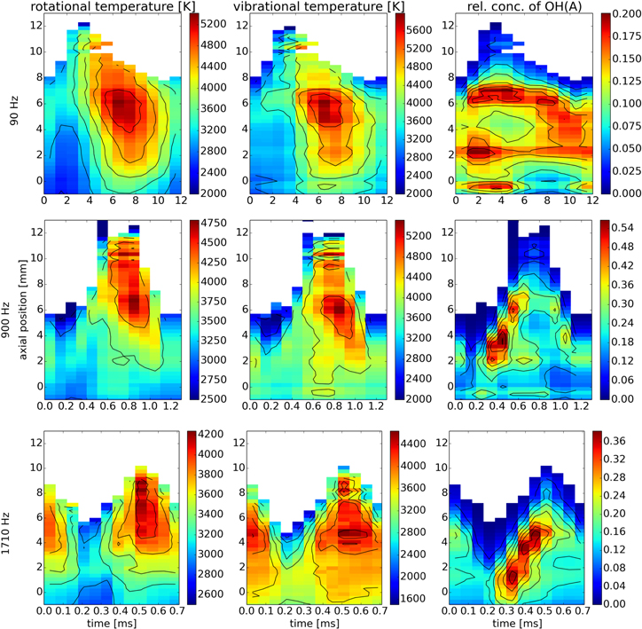
Figure 3. Maps of rotational and vibrational temperatures and relative concentration of OH (A). The isolated region of high relative concentration at the rising edge for the two higher frequencies marks the vortex ring, see [45].
Download figure:
Standard image High-resolution image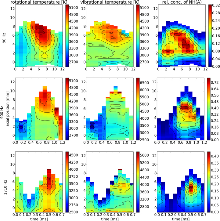
Figure 4. Maps of rotational and vibrational temperatures and relative concentration of NH (A).
Download figure:
Standard image High-resolution image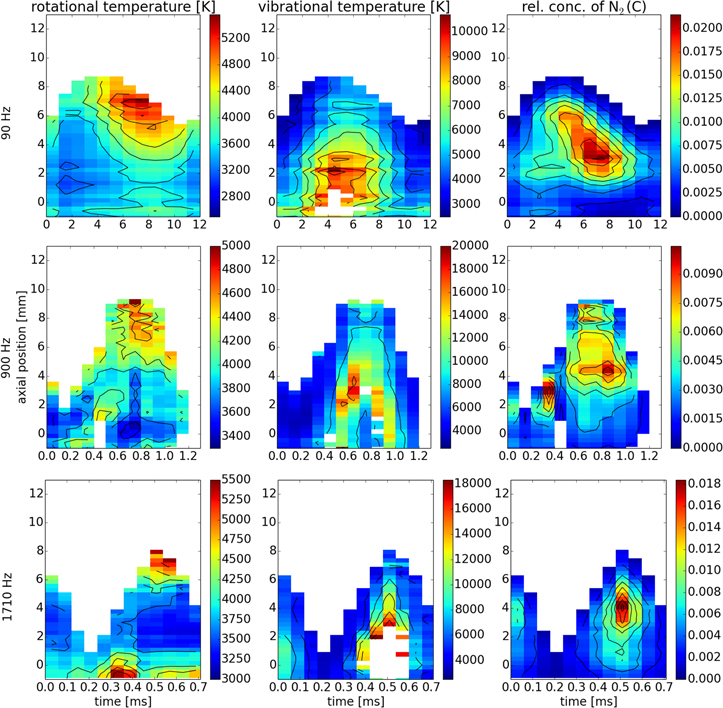
Figure 5. Maps of rotational and vibrational temperatures and relative concentration of N2 (C).
Download figure:
Standard image High-resolution image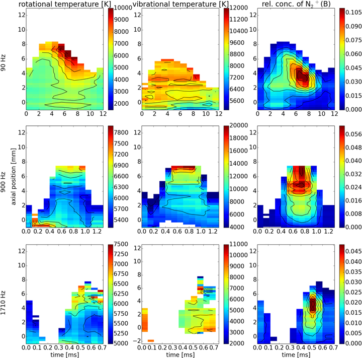
Figure 6. Maps of rotational and vibrational temperatures and relative concentration of  (B).
(B).
Download figure:
Standard image High-resolution image4. Results and discussion
Overview spectroscopy of the discharge was published in our previous publication [45] and spectra contained components from NO, NH, N2,  , H-Balmer series, O and Ar emission lines. In this article we have narrowed our focus to spectral regions which correspond to OH, NH, N2 and
  emission bands.
The calculated temperatures and relative concentrations for all four molecules and three modulation frequencies are shown in a streak-like form in figures 3–6. The two lighter molecules, OH and NH appear to share several characteristics. Most notably, all four temperatures ( ,
,  ,
,  ,
,  ) for a given set of conditions are in good agreement, which suggests that these molecules are close to thermal equilibrium. This may be rather surprising, concerning their origin: both NH and OH are formed in the discharge. The OH radical is in many cases found not to follow the Boltzmann distribution of rotational states [56–58]. The highly excited rotational states are often overpopulated and consequently, temperatures resulting from least-squares fit assuming the Boltzmann distribution tend to be exaggerated and do not reflect any real physical property of the discharge. However, closer look at figure 2 reveals that in this particular case, the otherwise often encountered OH anomaly was absent. Indeed, the highly excited rotational states are best observable in the P-branch, in the region (315–320) nm, where the fit reproduces the measured data as good as at the band head just below 310 nm. Straight Boltzmann plots shown in [44] further support this statement. The dissociative excitation of water molecules via its B
  state leading to overpopulation of highly excited OH rotational states, as discussed e.g. in [59], is apparently not a dominant process leading to OH(A-X) radiation in this type of discharge.
The NH radical is expected to be a result of recombination of N and H atoms. The rather scarce literature on NH in plasma [21, 60, 61] does not offer a comprehensive set of reactions leading to NH formation in atmospheric discharges. Detailed discussions of the process of formation and excitation of NH would thus be mere speculation. The fact that the measured NH temperatures are in such good agreement with temperatures of OH suggests that electronically excited NH(A) is either rapidly thermalised or that the observed emission comes from NH created previously in the discharge and excited later by electron impact, which tends to preserve the rotational distribution. In either case, it is highly probable, that the NH radical is created in three-body collisions, as otherwise the excessive energy after recombination would give rise to emission revealing its thermal inequilibrium with the surrounding gas.
The above discussed temperatures are also in good agreement with the rotational temperature of N2(C). Nitrogen is expected to be the most abundant molecular species in the discharge effluent and an overwhelming majority of excited N2 molecules is not resulting from any chemical reaction, but rather from an electron impact or collisions with argon metastables with lower states of N2. The rotational distribution of N2(C) is thus believed to be undisturbed by chemical processes and well represent the translational temperature of the gas Tgas. This together with the arguments above allows us to state that

The vibrational temperature of N2(C), however, differs significantly from Tgas. The maximal values of 10 000 K for 90 Hz and 20 000 K for faster modulations are several times higher than the maxima of Tgas around 5000 K. The measured vibrational temperature is very high indeed, but still insufficient for thermal dissociation of the N2 molecule, as the dissociation energy is over 9 eV [62]. Also, the maximal  appears earlier and closer to the surfatron plasma source compared to the maxima of Tgas. This can be explained as follows. The concentration of free electrons in this discharge was measured to be as high as 1020 m−3 during the whole modulation period [46]. The abundant electrons due to their low mass are much more efficient in exciting electronic and vibrational states of molecules (due to the Franck–Condon principle) compared to changing their rotational states. The heating of the gas (increasing the translational temperature) and increasing the rotational temperature takes place mostly indirectly during heavy particle collisions, where one of the collision partners was previously excited by electron impact. This energy redistribution is very rapid in OH [63] and NH [61]. N2, on the other hand, slowly gives the vibrational energy away. The preferred way seems to be a ladder-like vibrational deexcitation by one vibrational quantum at a time (see [64] and chapter 2 of [65]). This mechanism would certainly cause the molecules to keep the energy in the vibrational excitation and only reluctantly give it away to rotations and disordered translational motion [66]. The observed delay in gas heating after the rise of vibrational temperature of N2(C) is a natural consequence.
This kinetics is also responsible for the fact, that the highest observed Tgas is at the tip of the visible discharge (and perhaps even slightly rises further downstream, see [67]), as the chaotic translational motion is the final form of energy after the relaxation processes are finished. However, this fact alone does not explain why the main characteristics of the spatio-temporal temperature profiles only weakly depend on the modulation frequency.
Here, the tip of the discharge also plays a significant role as most of the power is absorbed at this region [68]. At the end of the conducting discharge channel, a sharp drop of electric potential, i.e. high electric field, is to be expected. Therefore, the electrons in this region are expected to absorb more energy from the microwave field and this affects the electronic, vibrational and in the end also rotational excitation of gas. During the sinusoidal power modulation, the discharge periodically elongates and shortens, the speed of this motion being the lowest in the turning points [43]. Consequently the time during which the gas continuously resides in this high absorption area decreases with the increase of frequency. During the rise of modulated power the discharge elongates, and the gas temperature is the lowest in all observed cases. After the power reaches its maximum value the discharge starts to shrink. In cases of 90 Hz frequency, this leaves a trail of high temperatures as the discharge tip subsides into already preheated areas. The same, yet slightly diminished effect can be observed for 900 Hz whereas for 1710 Hz temperature profiles are rather temporally symmetrical around power maxima.
An additional effect affecting the spatial temperature distributions should be mentioned. In our previous publication [45], we observed a vortex ring during the rising power at frequencies 900 Hz and 1710 Hz. The vortex ring was found responsible for shortening and widening of the visible discharge observed in [43]. It was also found, that the vortex can be easily tracked by strongly enhanced OH(A-X) (compare the higher frequencies to 90 Hz in figure 3). It can be observed that a region with lower gas temperatures is indeed introduced after the passage of the vortex ring. In the streak-like images of temperature, it is depicted as a sharper boundary at the bottom of the high temperature region as can be seen in figure 7. The effect of the vortex ring is, however, partially compensated by the rapid movement of the energetic discharge tip for the highest modulation frequency, leading to temperature homogenisation of the discharge effluent.

Figure 7. Maps of rotational temperature of OH (A-X) with a common scale. The black solid line in the last two images shows the region with enhanced OH emission, corresponding to the passage of the vortex ring. For 90 Hz, the vortex was absent.
Download figure:
Standard image High-resolution image
Unlike the three neutral molecules, the molecular ion  has significantly higher rotational and vibrational temperatures.
  is the only charged species investigated in this experiment. As already stated, the electron concentration in this discharge is as high as 1020 m−3. The cross sections for collision of charged species with electrons are significantly higher compared to neutral species due to the presence of the Coulomb interaction. In this respect, the proximity of
  temperatures to the temperature of electrons (which is around 1 eV in this type of discharge [36, 69]) is not very surprising.
The above-mentioned observations can be summarized to answer the question, how does the modulation influence the spatio-temporal characteristics of discharge? For 90 Hz we observe strong heating on the discharge tip and the streak-like maps of temperature are temporally asymmetrical with respect to maxima of power modulation. For 900 Hz this behaviour is less pronounced and appearance of vortex decreases temperature in the bottom part of the effluent. At 1710 Hz the streak-like temperature maps become temporally quite symmetrical and temperature gradients along effluent axis are much smoother. Generally, increases of modulation frequency leads to spatial and temporal averaging of temperature in the discharge where the maximum temperature drops while minimum temperature rises. We assume that further increases in the modulation frequency would lead to an increase in the degree of temperature homogenity.
5. Conclusions
Microwave plasma jet power modulated by sine envelope was operated in humid argon and blown into ambient air while spatio-temporally resolved optical emission spectroscopy was carried out in its effluent. The modulation induces changes in power transfer, fluid dynamics and plasma chemistry, opening possibilities for e.g. optimisation of plasma processing.
Our previous paper discovered the presence of a vortex ring at certain modulation frequencies in the 102–103 Hz range. The current paper extends this study further, using molecular spectra of OH, NH, N2 and  to calculate and discuss spatial and temporal distribution of rotational and vibrational temperatures.
The processing of large spectral datasets with overlapping molecular spectra necessitated a new approach. The resulting open source massiveOES software provides a tool to obtain rotational and vibrational temperatures and relative concentration for each species and is reasonably fast even during batch processing of such large datasets.
The spatio-temporal temperature profiles show that the vortex locally influences the gas temperatures but the frequency modulation plays a more important role in the temperature distribution along the whole axis of the plasma jet. Independently of modulation frequency the Tvib, Trot of OH and NH and Trot of N2 are almost equal which proves that the heavy species collisions dominate the energy transfer. However, the  temperatures (both Tvib and Trot) are much higher, closer to the electron temperature which can be explained by a much higher cross section of ion-electron collision than neutral-electron ones.
For the lowest modulation frequency of 90 Hz the gas temperature shows a high degree of variation along the time axis as the gas heating and heat dissipation are much faster than the changes induced by plasma modulation. The gas temperature reaches its peak values on the tip of the jet. Formation of vortex at 900 Hz leads to a spatially localized temperature drop as the vortex increases the heat transfer with surrounding gas. For 1710 Hz a homogenisation of gas temperature in both space and time is observed. We assume this is due to the fact that changes in plasma length are faster or on par with the heat transfer.
Acknowledgments
The authors acknowledge support of the project LO1411(NPUI) funded by Ministry of Education, Youth and Sport of Czech Republic.
The graphs in this publication were composed in the Matplotlib 2D graphics environment [70].
The authors are also grateful to Jean-Pierre van Helden for valuable discussions about the spectrum of NH radical.
Footnotes
- 1
Note, that the term 'relative concentration' is slightly inaccurate, as it neglects the effects of non-radiative manner (quenching, further excitation).
- 2
Again the concentration here does not consider effects of non-radiative manner like quenching, etc.
- 3
It is also usual for molecular spectra unless measured with an exceptionally high-resolution spectrometer.
- 4
Python scipy.optimize.leastsq() function, an implementation of the Levenberg–Marquardt algorithm, was used. The L-BFGS-B method [55] was found to be more robust at the cost of longer optimisation time.