
Abstract
We use atomic force microscopy (AFM) to perform a systematic quantitative characterization of the elastic modulus and dielectric constant of poly(L-lactic acid) electrospun nanofibers (PLLA), as well as composites of PLLA fibers with 1.0 wt% embedded multiwall carbon nanotubes (MWCNTs–PLLA). The elastic moduli are measured in the fiber skin region via AFM nanoindentation, and the dielectric constants are determined by measuring the phase shifts obtained via electrostatic force microscopy (EFM). We find that the average value for the elastic modulus for PLLA fibers is (9.8 ± 0.9) GPa, which is a factor of 2 larger than the measured average elastic modulus for MWCNT–PLLA composites (4.1 ± 0.7) GPa. We also use EFM to measure dielectric constants for both types of fibers. These measurements show that the dielectric constants of the MWCNT–PLLA fibers are significantly larger than the corresponding values obtained for PLLA fiber. This result is consistent with the higher polarizability of the MWCNT–PLLA composites. The measurement methods presented are general, and can be applied to determine the mechanical and electrical properties of other polymers and polymer nanocomposites.
Export citation and abstract BibTeX RIS

Content from this work may be used under the terms of the Creative Commons Attribution 3.0 licence. Any further distribution of this work must maintain attribution to the author(s) and the title of the work, journal citation and DOI.
1. Introduction
Polymer nanocomposites constitute very promising, cost effective candidates for applications in a variety of fields, such as mechanical engineering, nanoscale electronics, chemical sensing, tissue engineering and biosensing [1–6]. These materials typically consist of a polymer matrix which embeds one or several types of nanofillers (e.g., nanoparticles, carbon nanotubes (CNTs), or nanoplatelets etc).
Due to their remarkable physical properties (large aspect ratio, mechanical strength, high polarizability, increased thermal conductivity etc) CNTs represent one common type of nanofiller used to tune the electrical, mechanical, thermal and optical properties of the polymer composite [7–12]. For example, by controlling the concentration and orientation of CNTs in poly(lactic acid) (PLA) fibers researchers have created nanocomposites with improved properties for naonelectronics [7, 8], biosensing [13], and tissue engineering applications [6]. PLA is a chiral polymer with two optical isomers: poly(L-lactic acid) (PLLA) and poly(D-lactic acid) (PDLA). Both isomers have well-understood degradation and biocompatible properties, and form high strength polymers that can be electrospun into fibers with controllable diameter ranging from tens of nanometers to microns. Since the physical properties of the polymer nanocomposite are very sensitive to the concentration and spatial distribution of CNTs it is critical to have non-invasive techniques that enable the characterization of these subsurface structures with high sensitivity and high spatial resolution. While both scanning electron microscopy and transmission electron microscopy have the necessary resolution, they typically require sample preparation steps that could potentially change or damage the sample. In addition, the high energy electrons in the beam can damage the polymer matrix.
Several techniques based on the atomic force microscope (AFM) have been used for non-invasive, high resolution characterization of topographical and electrical properties of polymer/CNT nanocomposites. For example, electrostatic force microscopy (EFM) has been used for subsurface imaging of CNTs dispersed in thin films of poly(methyl methacrylate) [14], or suspended in polyimide nanocomposites [15]. EFM has also been applied to image and characterize dielectric properties of poly(ethylene oxide) (PEO) and doped polyaniline/PEO nanofibers [16]. Other AFM—based techniques such as scanning impedance microscopy [17] and dc-biased multifrequency dynamic AFM have been used for high resolution imaging of two- and three-dimensional networks of CNTs underneath polymer matrices [18, 19].
Here we use AFM force compression experiments (the force–volume mode of the AFM) to measure mechanical properties in the fiber skin region and acquire systematic, high-resolution elasticity maps for two types of polymers formed by electrospinning: PLLA nanofibers and multi-walled carbon nanotube—polylactic acid (MWCNT–PLLA) composite nanofibers. We find that the transverse elastic moduli of the MWCNT–PLLA composites are significantly lower than the corresponding elastic moduli of PLLA fibers of similar diameter. MWCNT–PLLA composite fibers also display an increase in the elastic modulus with increasing fiber diameter, a trend which is not observed for neat PLLA fibers. We also use EFM to measure dielectric properties of both PLLA and MWCNT–PLLA fibers, and demonstrate that these experiments allow us to clearly distinguished between the dielectric constants for the two systems. MWCNT–PLLA composites display larger dielectric constants compared to PLLA fibers, consistent with a higher polarization of these composites.
2. Materials and methods
2.1. Preparation of PLLA fibers and MWCNT–PLLA composites
In this study we have used PLLA 3051D manufactured by NatureWorks in pellet form. Hexafluoro-isopropanol from Oakwood Chemical was used as solvent with a concentration of 10 wt% solid content for electrospining. MWCNTs (MER Corporation) used in these experiments have a quoted diameter range: 90–290 nm. MWCNTs were purified by adding them to a mixture of concentrated sulfuric acid and nitric acid (at 3:1 volume ratio). The solution was sonicated in a Misonix water bath sonicator for 24 h at 323 K to separate the MWCNT bundles. The resultant suspension was next diluted with deionized water and filtered through a 400 nm pore membrane (PTFE) until the water passing through the filter had a pH between 6 and 7. Finally, the dispersions were filtered to the desired concentration. The recovered MWCNTs were then mixed together with PLLA to form sparsely loaded composites, at a weight content 1.0 wt% MWCNTs relative to the PLLA weight. The solution was stirred overnight at room temperature before being filled into a glass syringe.
Electrospinning was done at room temperature with a working distance of 12 cm measured from the tip of the syringe needle to the grounded collector. The high voltage power supply (Gamma High Voltage Research Inc. Model no. ES30P-5w) provided an applied voltage of 15 kV. Polymer solvent was ejected as a droplet from a syringe needle of inner diameter 1.194 mm at a flow rate of 0.06 ml min−1 then accelerated by the action of electric field and finally deposited as fibers on the rotating grounded collector drum [20–22]. The rotation speed was 2000 rpm which allowed us to get aligned fibers deposited on the substrates. The substrate for all experiments is a 400 nm SiO2 layer on top of a p-type degenerately doped Si wafer. To obtain rarefied fibers for AFM studies, the collecting time was set at 10 s. Longer collection times (ca. 1 h) were used to obtain dense non-woven fibrous mats, for other testing like differential scanning calorimetry, wide-angle X-ray diffraction, and dynamic mechanical analysis [21, 22, 30]. After electrospinning, all samples were put into a vacuum oven to dry for 24 h before further testing. Representative scanning electron microscope images of the PLLA and MWCNT samples are shown in supplementary figure 1. All SEM images were acquired on a Phenom Pure SEM at Tufts University. In addition, neat PLLA cast film and bare MWCNTs were examined to serve as samples for control experiments.
2.2. AFM and EFM measurements
AFM topographical imaging, force mapping and EFM measurements were collected using an Asylum Research MFP3D AFM (Asylum Research, Santa Barbara, CA), integrated with an inverted Nikon Eclipse Ti optical microscope (Nikon, Inc.). All measurements were taken using Olympus Cantilevers (AC160TS Asylum Research/Oxford Instruments, Santa Barbara, CA) with a calibrated spring constant of k = (42 ± 10) N m−1 and radius of curvature R = (9 ± 2) nm. The spring constant was measured using the thermal calibration built in to the MFP3D software of the AFM. Along each fiber we measured three different regions, separated by 5–10 μm. For each region we acquired a 2 × 2 μm map of individual force versus indentation curves, with a resolution of 100 nm between points (for fibers with diameter <100 nm this means that there is one data point collected across the diameter, i.e. all data points are collected along the fiber length). The total number of data points measured on each fiber varies between 30 and 100, depending on the fiber diameter. To limit energy dissipation due to viscoelastic effects the cantilever z velocity was kept at 1 μm s−1, with a maximum cantilever deflection of 30 nm. The elastic modulus values were determined by fitting the Hertz model for a 30° conical indenter to the acquired force versus indentation curves using the Asylum Research MFP-3D Hertz analysis tool (force–volume mode). To extract the elastic modulus from force versus indentation curves the MFPD-3D analysis tool uses Sneddon's modification of the Hertz contact model for a 30° conical indenter [23]:
where F is the applied force, E is the elastic modulus, α is the half-angle of the conical indenter, δ is the indentation depth, and ν = 0.5 is the Poisson ratio. These values can be combined with surface height information to produce a topographical rendering with elastic modulus values mapped on the surface (figure 1). EFM measurements were performed using Olympus Ti/Pt coated electriLevers (AC240TM, Asylum Research/Oxford Instruments, Santa Barbara, CA) with spring constant k = (2 ± 1) nN nm−1 and tip radius R = (30 ± 10) nm.
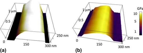
Figure 1. (a) Three-dimensional AFM image of a segment of a PLLA nanofiber. The length of the segment is 1 μm, and the fiber average diameter is 225 nm. The color plot shows the map of the compressive elastic modulus on the fiber measured using the force–volume mode of the AFM. The fiber average elastic modulus is (11.2 ± 0.7) GPa. (b) Three-dimensional AFM image of a segment of a MWCNT–PLLA nanofiber. The length of the segment is 1 μm, and the fiber average diameter is 215 nm. The color plot shows the map of the compressive elastic modulus on the fiber measured using the force–volume mode of the AFM. The fiber average elastic modulus is (4.4 ± 0.5) GPa. The color scale bar on the right is the same for both nanofibers.
Download figure:
Standard image High-resolution image3. Results and discussion
3.1. AFM topography and AFM force–volume measurements of PLLA and MWCNT–PLLA nanofibers
Figures 1(a) and (b) show three-dimensional topographical images for two segments of a PLLA and MWCNT–PLLA nanofiber, respectively. The color plots in these images show the distribution of the compressive elastic modulus on each fiber, measured as described in section 2. We note that the diameter, topographical features and the distribution of elastic modulus maps are similar for both types of nanofibers. However, the average value for the elastic modulus measured on the MWCNT–PLLA nanocomposite is significantly lower than the corresponding value for the PLLA nanofiber. We find that this result holds for all fibers that we have measured, independent of the fiber diameter (n = 14 PLLA fibers and n = 22 MWCNT–PLLA fibers). A summary of all these measurements is shown in figure 2, which displays the average value for the elastic modulus measured on each fiber as a function of the fiber diameter. The red squares in this figure represent data points measured on PLLA nanofibers, while the black squares represent data points measured on MWCNT–PLLA nanocomposites. We note that the average values of the elastic modulus obtained for the PLLA fibers (red squares in figure 2) are larger than the values obtained for PLLA films (E ∼ 3 GPa, supplementary figure 2 and [5, 24–26]). Gupta et al [26] report that hot drawn fibers could have tensile moduli as high as 9.2 GPa, a result supported by theoretical calculations of Montes de Oca and Ward [5] for the transverse elastic moduli for cylindrically symmetric PLLA crystals. Our results may be explained by formation during electrospinning of fibers with high molecular chain alignment at the surface of the fiber (shown in figures 3(a) and (b)), leading to an oriented amorphous mesophase recently measured by our group for PLA neat fibers [22].
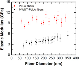
Figure 2. Plot of the measured elastic modulus versus nanofiber diameter for nanofibers of PLLA (red squares) and MWCNT–PLLA (black squares). Elastic moduli are measured using the force–volume mode of the AFM. Three different regions, separated by 5–10 μm were measured along each fiber. For each region we acquired a 2 × 2 μm map of individual force versus indentation curves, with a resolution of 100 nm between points. The total number of data points measured on each fiber varies between 30 and 100, depending on the fiber diameter. The error bars are obtained from the standard deviation of the mean for these data points. The average elastic modulus for all PLLA fibers (n = 14) is: (9.8 ± 0.9) GPa. The average elastic modulus for all MWCNT–PLLA fibers (n = 22) is: (4.1 ± 0.7) GPa.
Download figure:
Standard image High-resolution image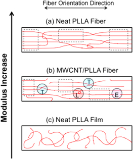
Figure 3. Schematic of the sample cross-section for the top 30 nm of the sample, subject to the indentation force of the AFM tip. Red lines depict the polymer molecular chains within the fiber or film. The horizontal arrow indicates the orientation direction of the fibers. (a) Neat PLLA fiber. (b) MWCNT‐PLLA fiber. The carbon nanotube is not shown in the schematic, because it lies below the detection distance of the AFM tip. (c) Amorphous neat PLLA film. In (a) and (b), regions which can form an amorphous mesophase are outlined with dashed boxes. In (b), highlighted circles show examples of chain ends (E), and molecular entanglements including tie molecules (T), and loops (L).
Download figure:
Standard image High-resolution imageFigure 2 also shows an increase in the average elastic modulus with the fiber diameter for MWCNT–PLLA fibers. No such dependence is observed (within the experimental uncertainties) for neat PLLA fibers. We have used the AFM-force volume mode of the AFM to measure the transverse elastic modulus of the bare MWCNTs (supplementary figure 3) and found an average value of (21 ± 3) GPa. This result is consistent with measurements reported in literature for MWCNTs of smaller diameter [27]. Although the embedded MWCNTs have a larger elastic modulus than the host PLLA fibers, they are sparsely loaded into the fibers forming a core–shell structure. Most of the fiber volume is empty of MWCNTs, and the data in figure 2 can be explained by existence of an amorphous phase of lower elastic modulus at the surface of the MWCNT–PLLA composite depicted in the model of figure 3.
In polymer films and fibers, stress is transferred throughout the material via chain entanglements (in figure 3, tie molecules and loops), which are topological constraints on chain mobility. Higher entanglement density results in better stress transfer and high modulus; lower entanglement density results in weak stress transfer and low modulus. We suggest the effect of MWCNT addition is to reduce the polymer chain entanglement density during fiber formation.
Figure 3 is a model of presumed molecular chain structures of neat PLLA fiber (a), MWCNT–PLLA fiber (b), and neat PLLA film (c). The model shows only the top 30 nm of the shell region in cross-section, from which the elastic moduli are obtained by the AFM tip indentation. The neat PLLA film has the lowest elastic modulus, and contains amorphous polymer chains randomly arranged as Gaussian coils. Electrospinning of the fiber results in highly oriented and entangled molecular chains in both the MWCNT–PLLA and neat PLLA fibers. The effect of adding conductive MWCNTs into the electrospinning solution is to increase the flight speed of the fibers from the needle to the collector, causing the composite fibers to be more highly stretched by the electric force. In our model, we suggest that polymer chain stretching results in more polymer chain disentanglement (or more chain ends in figure 3(b)) within the skin region for the composite fibers, compared to their neat counterparts. This results in lower elastic modulus in the skin region. As the overall fiber diameter increases, the exterior skin portion is less affected by the embedded MWCNT leading to a steady increase in number of entanglements as fiber thickness increases.
As shown in figure 3(a), the molecular chains exhibit a higher degree of entanglement in the neat PLLA fibers, and fewer disentangled chain ends (E). Entanglements (physical cross-links) such as tie molecules (T) and loops (L) serve to prevent slippage of the molecular chains along the fiber direction during electrospinning. The model also depicts regions of an amorphous mesophase (outlined with dotted boxes) showing highly parallel molecular chains without three-dimensional crystalline order, a feature which we measured in previous studies of PLLA electrospun fibers [22]. We suggest that electrospinning MWCNT–PLLA results in greater disentanglement (fewer tie molecules and loops) resulting in a lower modulus in the shell region of the fiber compared to its neat PLLA counterpart. This model is consistent with the data in figure 2, which shows that the transverse elastic modulus E of the MWCNT–PLLA composites is a factor 2–3 less than the corresponding elastic modulus for PLLA fibers of comparable diameter D. This conclusion is further supported by the observed increase in the transverse elastic modulus with the fiber diameter for MWCNT–PLLA composites (figure 2, black squares). As the fiber diameter increases, the fibrillar arrangement of the PLLA molecular chains is less affected by the polymer interaction with the coaxial MWCNT, i.e. the AFM tip probes a more ordered and entangled PLLA fiber. In the limit of large fiber diameter we thus expect to obtain values of the elastic modulus for MWCNT–PLLA composites that approach the corresponding values measured for the PLLA fibers.
3.2. EFM measurements of PLLA and MWCNT–PLLA nanofibers
To gain a deeper quantitative understanding of the dielectric properties of PLLA and MWCNT–PLLA nanocomposites we perform EFM measurements of both types of fibers. EFM is a dual-pass AFM technique [16]. In the first line scan the AFM-tip acquires the topography profile of the sample in tapping mode (figures 4(a) and (b)). In the second line scan, the tip travels at a preset height above the sample surface (h = 50 nm for the experiments presented here). During the second pass the AFM cantilever is excited electrically by applying a dc voltage Vdc, and the AFM cantilever is driven at its resonant oscillation frequency (ω0 ≈ 75 KHz, in our experiments). Both the cantilever oscillation frequency and the oscillation phase change due to the electrostatic interactions between the voltage—biased AFM-tip and the sample. The EFM image records the phase of the cantilever oscillation as a function of the tip position (figures 4(c) and (d)).
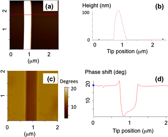
Figure 4. (a) AFM topographic image of a segment of a PLLA nanofiber. (b) Line scan (cross-section) along the red line shown in (a). The fiber diameter is 200 nm. (c) EFM (phase) image of the same segment of PLLA nanofiber shown in (a). (d) Line scan along the red line shown in (c). The line scan shows a negative phase shift when the tip scans above the PLLA fiber, which is due to the electrostatic interaction between the tip and the sample. The positive phase shift as the tip is approaching the fiber (from the left) is an effect of the cross-talk with the topography channel, and is explained in the text.
Download figure:
Standard image High-resolution imageFigure 4(a) shows typical AFM-topography image of a neat PLLA sample, while figure 4(b) shows a cross-section (line scan) used to measure the fiber diameter. Figure 4(c) displays the corresponding EFM image acquired of the same region of the PLLA fiber as the topography shown in figure 4(a). We explain these images quantitatively by modeling the AFM cantilever as a driven harmonic oscillator of resonant frequency ω0, quality factor Q and spring constant k. If the cantilever is scanned at height h above a bare SiO2 substrate, the electrostatic force  between the metallic tip and the surface changes the cantilever resonant frequency, which leads to a constant shift in the oscillation phase (background phase in figures 4(c) and (d)) [16]:

where Vdc is the tip voltage, and  is the second derivative of the tip-sample capacitance with respect to tip position h. When the tip is above the sample (PLLA nanofiber, MWCNT–PLLA composite etc) the total capacitance of the system is
  with electrostatic force
  We note that the tip stays at the same height h above the sample since it retraces the topography. This interaction leads to an additional phase shift (relative to the bare substrate) given by [16]:

Equations (2) and (3) predict that the tangents of both the phase background value and the phase shift above the fiber vary linearly with  This is indeed seen in the data taken above the bare SiO2 substrate and bare PLLA fibers (see supplementary figure 4).
In addition to the main (negative) phase shift observed over the fiber the EFM image shows a positive phase shift, measured as the tip approaches the nanofiber (tip motion is left to right in figure 4). Figure 5 shows two examples of phase shifts measured over the same line scan, as the AFM-tip scans from left to right in figure 5(a) (AFM trace), or right to left in figure 5(b) (AFM retrace). The fact that this phase contrast changes position with respect to the fiber depending on the scan direction shows that it is an artifact of cross-talk from the topography signal. To explain this positive peak in the phase shift we note that as the tip approaches the nanofiber at height h above the substrate, two forces act on the cantilever: the capacitive force from the tip–substrate (interaction F1) and an additional attractive force Ftf due to the tip–fiber interaction. This additional force leads to a increase in the absolute phase shift Φ (from equation (2),  >
>  and thus to a positive phase shift ΔΦ. When the tip is directly above the fiber, the phase shift is due to the capacitive coupling between tip and nanofiber (equation (3)). Since the diameter of the metallic fiber (D = 50 – 300 nm) is larger than the tip radius in a first approximation we can model the tip and sample as a sphere above a plane, and find that
  for all scan heights h = 10 – 500 nm, leading therefore to a negative shift above the metallic fiber. Although this model explains qualitatively the positive–negative variation of the phase shift, the numerical predictions do not agree with the data, which is to be expected since the tip radius R = (30 ± 10) nm is comparable with the fiber diameter, and the system cannot be modeled as a sphere above a plane. This suggests that the geometry of the tip should be taken into account in order to extract quantitative information from the EFM measurements. This model is discussed in the next section.

Figure 5. Example of phase shifts measured over the same scan line in: AFM trace (a), and retrace (b). The images show that the same negative phase shift (measured with respect to the background) is observed over the PLLA fiber. However, the positive phase shift (with respect to the background) switches positions and is always observed on that side of the fiber which the AFM tip approaches first (indicated by the arrow). This indicates that this 'positive' phase shift is an image artifact due to the cross-talk with topography channel. The blue circles represent the AFM cursor.
Download figure:
Standard image High-resolution image3.3. Measurement of the dielectric constants for PLLA and MWCNT–PLLA samples
For a conical tip of half angle θ the second derivative of the AFM tip–substrate capacitance is given by [15]:
where  F m−1 is the vacuum permittivity,
  S = 3.9 is the SiO2 dielectric constant, and t represents the thickness of the SiO2 layer (400 nm in our experiments). Similarly, the second derivative of the AFM tip–nanofiber capacitance is [15]:

where D, f are the PLLA (or MWCNT–PLLA) fiber diameter and dielectric constant, respectively.
We are using the negative phase shift measured from EFM images and the model described by equations (3)–(5) to measure the dielectric constant for both types of nanofibers: PLLA and MWCNT–PLLA. The histograms in figure 6 show the distribution of dielectric constants obtained from EFM images for PLLA fibers (n = 30, figure 6(a)) and MWCNT–PLLA fibers (n = 30, figure 6(b)).

Figure 6. Histograms showing the distributions of the dielectric constants obtained for PLLA nanofibers (a) and MWCNT–PLLA nanocomposites (b). An equal number of fibers (n = 30) was measured in both cases. On the EFM image for each fiber, the phase shift was measured for a number of 20–30 line scans. The fiber dielectric constant was then calculated from the measured phase shifts for each line scan using equations (4)–(6) and a Mathematica script. The histograms show the distributions of the dielectric constants obtained for all line scans. The two distributions are clearly distinct. This is further confirmed by the one-way ANOVA significance test (p < 0.001).
Download figure:
Standard image High-resolution image
Figure 6 shows that the two types of nanofibers have clearly distinct dielectric properties. The average value for the PLLA dielectric constant obtained from the data shown in figure 6(a) is:  which is close to the values obtained on PLLA films [4]:
  The average value for MWCNT–PLLA dielectric fibers obtained from the data in figure 6(b) is:
  The higher dielectric constant obtained for the MWCNT–PLLA nanofibers is consistent with a higher transverse polarizability of these nanocomposites due to the presence of multi wall CNTs [8, 11]. EFM measurements performed on bare MWCNT allow us to directly measure the (transverse) dielectric constant for the nanotubes:
  (supplementary figure 3). We note that this is consistent with dielectric constants reported in literature for metallic nanotubes of smaller diameter [28].
In principle, the dielectric constant of a composite material can be calculated from the known values of the homogeneous components using the effective medium theory [29]. Within this approximation, we obtain the following relation between the transverse dielectric constants for PLLA fibers, MWCNT and the MWCNT–PLLA composite:

where p1 and p2 are the volume fractions of the PLLA and MWCNT respectively. Using the measured dielectric constants and equation (6) we obtain an average ratio between the volume fractions:  We emphasize that this relation is valid for the transverse dielectric constants measured in our experiments, and therefore the average ratio of the volume fractions in equation (6) is also proportional to the ratio between the cross-sectional area of the PLLA fiber and MWCNT in the composite, i.e. in the cylindrical (core–shell) approximation we have:
where Dcomp and DCN represent the average diameter of the MWCNT–PLLA composites and the average diameter of the MWCNT respectively. Given the distribution of average diameters in our samples  equation (7) predicts an average value for the transverse volume fractions:
  in agreement with the value obtained from equation (6). We thus conclude that the measured values of the dielectric constant for the PLLA fibers, MWCNT and MWCNT–PLLA composite fibers are in good agreement with the prediction of a simple core–shell model for the composite, where the MWCNT is aligned along the fiber axis and surrounded by PLLA polymer. Electrical measurements thus provide independent confirmation for this simple model, which also explains the mechanical measurements and the observed variation in elastic modulus with fiber diameter.
4. Conclusions
We have used AFM and EFM to measure mechanical and dielectric constants for two different types of polymers: PLLA nanofibers and MWCNT–PLLA nanocomposites. We find that the compressive elastic modulus in the fiber skin region for PLLA fibers is larger by a factor of two compared to the corresponding elastic modulus for MWCNT–PLLA composites. We explain this difference by a simple core–shell model where the CNT is aligned along the fiber axis. This model also predicts the formation of a mesophase introduced by alignment of molecular chains, in the shell region of the polymer-CNTs composites. The EFM data, combined with a theoretical model that describes the interaction between the AFM-tip and the nanofibers, have been used to measure dielectric constants for both types of fibers. These measurements show that the average dielectric constant of the MWCNT–PLLA fibers are significantly larger than the corresponding value obtained for neat PLLA fibers. This result is consistent both with the higher polarizability of the MWCNT and with the core–shell model proposed in the mechanical measurements. We anticipate that these quantitative, AFM-based techniques will be very useful as high-resolution, non-destructive tools for measuring mechanical properties and dielectric constants of nanocomposites with a broad range of applications in nanotechnology.
Acknowledgments
The authors thank Professor Georgiev (Assumption College) for providing purified MWCNTs and Professor Ayse Asatekin (Tufts U) for use of the Phenom SEM and plasma deposition equipment. This work was supported by the Tufts Faculty Research Award (FRAC) (PB, QI) and by the National Science Foundation, Polymers program of the Division of Materials Research, through DMR-1206010 and Division of Biomedical Engineering, through CBET 1067093.