

Abstract
RainbowPIV is a recent imaging technology, proposed for time-resolved 3D-3C fluid velocity measurement using a single RGB camera. It dramatically simplifies hardware setup and calibration procedures as compared to alternative 3D-3C measurement approaches. RainbowPIV combines optical design and tailored reconstruction algorithms, and earlier preliminary studies have demonstrated its ability to extract physically constrained fluid vector fields. This article addresses the issue of limited axial resolution, the major drawback of the original RainbowPIV system. We validate the new system with a direct, quantitative comparison with four-camera Tomo-PIV on experimental data. The reconstructed flow vectors of the two approaches exhibit a high degree of consistency, with the RainbowPIV results explicitly guaranteeing physical properties, such as divergence free velocity fields for incompressible fluid flows.
Export citation and abstract BibTeX RIS

Original content from this work may be used under the terms of the Creative Commons Attribution 4.0 license. Any further distribution of this work must maintain attribution to the author(s) and the title of the work, journal citation and DOI.
1. Introduction
In recent years, a great deal of effort has been invested into the development of methods for the complete volumetric reconstruction of three-dimensional, three-component (3D-3C) velocity vector fields. Tomographic Particle Imaging Velocimetry (Tomo-PIV) [4, 17] has long been considered the standard technology for 3D measurement, due to its ability to handle high particle seeding densities and high spatial resolution reconstruction, as well as its robustness to many types of flow phenomena. Recent advances in Tomo-PIV technology have included improved reconstruction accuracy [10, 12], spatial and temporal resolution [18, 19] by exploiting temporal information, and reducing the cost of setup, e.g. using smartphones [1, 3]. Tomo-PIV typically makes use of 4–6 cameras, capturing the volume of interest from different viewing angles. While Tomo-PIV has the advantages mentioned above, it also suffers from several limitations that constrain its use. Firstly, a considerable amount of effort is required to set up and calibrate a multi-camera system. Precise calibration is required, to prevent degradation of the reconstruction quality. Depth-of-field is another practical issue limiting its applications; achieving a large depth-of-field requires a small numerical aperture, which leads to low light efficiency (using a powerful light source is expensive and carries potential safety issue). Another severe limitation is that there are many experimental setups where optical access is limited; in such situations, setting up a multi-camera system becomes impractical, and a single-camera based 3D-3C technology would be more appropriate.
Two main types of single-camera approaches have been proposed for 3D flow measurement: encoding particle depth into the light path on the camera side, or into color or spectral information on the illumination side. The strategy of encoding particle depth by light path dates back to the work of Willert et al [24], who placed a three-pinhole mask in front of the objective, recovering 3D particle locations based on the position and length of captured image patterns (equilateral triangles) by means of a defocusing technique. This method has been applied to several flow scenarios [13, 27], although it has the disadvantage of low light efficiency (given that most of the light is blocked by the pinhole mask), as well as low particle seeding density due to the difficulty of distinguishing overlapping patterns from nearby particles. More recently, single-camera PIV approaches, based on plenoptic (or light-field) cameras, have been proposed [5, 21]. These record the full 4D light field of the scattered light of seeding particles, and digitally reconstructs particle locations by means of ray-tracing based algorithms. Quantitative comparisons between Tomo-PIV and Plenoptic-PIV have been conducted in recent studies [15, 20]. Plenoptic-PIV dramatically simplifies the hardware setup and gets rid of the complicated calibration procedures required for Tomo-PIV. On the other hand, significant spatial resolution is sacrificed in favour of angular information with this approach. In addition, the available plenoptic cameras suffer from comparatively low frame rates, which in turn limits the usefulness of this approach for time-resolved non-stationary fluid flow measurements.
Another group of single-camera methods is based on the encoding of particle depth by structured light (monochromatic or polychromatic light). Here, the 3D particle locations can be determined by 2D spatial location and 1D illumination information in a single captured image. A method for exploiting monochromatic illumination has been proposed in [2], which illuminates the volume by a spatially and temporally varying intensity profile, and achieves an axial resolution of 200 discrete depth levels. However, temporal resolution is sacrificed to a certain extent for the sake of high depth resolution, and the method also fails to separate overlapping particles. Most of the related work involving the use of polychromatic illumination is summarized in [23]. Early works extracted data relating to particle depth based on a calibrated mapping function of RGB, or hue value to depth. This naive method cannot deal with overlapping particles, and making it unsuitable for dense fluid flow reconstructions. An additional disadvantage is that the method is sensitive to random noise, optical aberrations, and unpredictable secondary light scattering from the particles.
The recently proposed RainbowPIV [26] tackles most of the existing issues by virtue of a joint design between the measurement setup (illumination and camera optics), and the reconstruction software. The measurement setup of RainbowPIV consists of an illumination module to generate a rainbow pattern, which color-codes the distance of particles from the camera, as well as a diffractive optical element in front of the camera lens, which provides all-in-focus imaging of the color-coded particles. The reconstruction software comprises an integrated optimization framework to jointly reconstruct both particle distributions and velocity vector fields.
Many single-camera methods suffer from a limited depth-to-width ratio, i.e. they can image only shallow volumes. Indeed, the initial RainbowPIV system [26] had such a limited depth-to-width ratio, which was fixed at 0.36. However, in principle, the volume depth in RainbowPIV can be tuned by a) altering the thickness of the rainbow, and b) adjusting the design of the all-focus camera optics. This was demonstrated in [25], which proposed a reconfigurable RainbowPIV system with an adjustable rainbow generation engine and a varifocal optical design, extending the depth range to (15–50 mm), while the lateral resolution is unaffected. This corresponds to a depth-to-width ratio of 0.3 - 1. Unfortunately, extending the depth range in this fashion reduces the depth resolution, as the same number of distinguishable depth layers are spread out over a larger range.
Therefore, despite the advantages of Rainbow PIV in terms of simplicity of setup, it still suffers from a limited axial resolution compared to multi-camera methods such as Tomo-PIV. In this work, we address this issue, and propose an extension to the precedent RainbowPIV by implementing a depth super-resolved RainbowPIV system. Furthermore, we carry out a direct comparison with the well-established four-camera Tomo-PIV system, so as to verify its applicability and reconstruction accuracy for flow measurement. Moreover, we demonstrate that RainbowPIV, unlike Tomo-PIV, reconstructs physically plausible flows, e.g. divergence-free flow fields for incompressible fluid flow.
2. Experimental setup
In order to realize a simultaneous measurement for both RainbowPIV and Tomo-PIV, the schematic diagram for the designed experimental setup is shown in figure 1. Four identical color cameras (RED SCARLET-X DSMC with sensor MYSTERIUM-X (30 mm × 15 mm, 4096 × 2160 pixels) are arranged to view an octagonal tank from different perspectives for Tomo-PIV. The elevation angle between camera 2 and 3 is 15°. The internal clocks of the four cameras and triggering signals are produced with the time code generator 'Lockit ACL 204'. The central bottom camera (camera 3), equipped with a specially designed diffractive optical element (DOE) to form a hybrid refractive/diffractive imaging system, is also utilized for RainbowPIV. The DOE is a Fresnel phase plate, and is used for all-in-focus imaging in the RainbowPIV setup. In general, the cameras used in a Tomo-PIV setup use a relatively small aperture size in order to obtain a greater depth-of-field. The resulting loss in light efficiency presents additional practical challenges, particularly in relation to high speed fluid imaging applications. In contrast, the depth-of-field of the utilized hybrid refractive/diffractive lens is not affected by the aperture size; as a result, RainbowPIV can make use of the largest available aperture for maximum light efficiency while still maintaining an extended depth-of-field. Specifically, in our setup, the camera with DOE uses an aperture of f/1.8 (the maximum aperture), while the remaining cameras use f/5.6 to achieve a good balance between depth-of-field and light efficiency. The design, fabrication and impact of the DOE are explained in detail in [26].
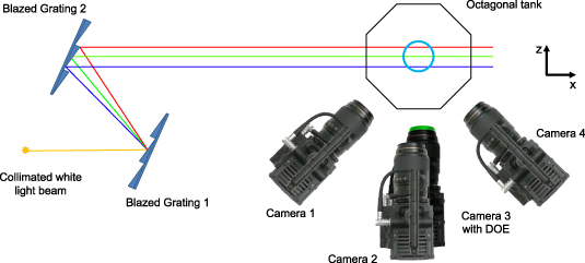
Figure 1. Schematic diagram for the experimental setup. Two blazed gratings are used to generate a size-controlled rainbow. Four cameras are utilized for Tomo-PIV measurement, of which the third camera, with custom designed DOE (diffractive optical element) for all-in-focus imaging, is also used for RainbowPIV.
Download figure:
Standard image High-resolution imageAnother notable element is the illumination system (rainbow generation). The physical size of the measured volume is dependent on the field-of-view of the camera (x-y) and the illumination width (z), corresponding to the rainbow width. In order to generate a collimated rainbow beam with a controllable depth, we utilize two blazed gratings and place them parallel to each other at the blazing angle. A white light beam (produced by a Sumita LS M350 light engine with a power consumption of 450 W) entering the setup is separated into a collimated set of monochromatic light sheets, forming a rainbow. The thickness of this rainbow can be adjusted by altering the distance between two gratings. In the experiment, we work on a 25 mm rainbow with wavelength ranging from 480 nm to 680 nm. The size of the x-y plane observed by the camera is 50 mm × 35 mm.
White Polyethylene Microspheres, with a diameter in the range [90, 106 µm] are used in the experiments. We place a vortex ring generator (figure 2) beneath the tank to produce specific flow scenarios for measurements. This is composed of a cylindrical chamber, with an elastic latex membrane in the lower third. At the top, the cylinder is covered with a 3D printed cap with a circular aperture. An air pulse enters the bottom chamber and pressurizes the membrane upwards, driving water out of the top chamber through the aperture, and finally generating the desired vortex rings.
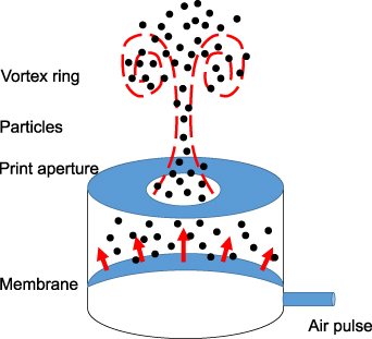
Figure 2. Schematic diagram for the vortex ring generator.
Download figure:
Standard image High-resolution imageFor Tomo-PIV processing, by converting the RGB images to 8-bit grayscale images, a 1120 × 780 × 560 particle intensity field is reconstructed using the MART method, followed by a multi-pass cross-correlation with reduced interrogation window size and 75% overlap. The reconstructed velocity field has a size of 50 × 35 × 25, resulting in a spatial resolution of 1 mm along all 3 axes. All of the algorithms employed here are constructed using LaVision Davis software.
3. RainbowPIV tracking and reconstruction
3.1. Joint optimization framework
In order to fully reconstruct dense 3D-3C velocity fields, prior work has utilized a pipeline approach that first estimates the particle distribution fields at successive time steps, and then reconstructs the corresponding flow fields using the estimated particle distributions. Separating particle distribution field and velocity field reconstructions neglects temporal coherence as a strong physical cue. Specifically, particles present at one time step should also be present at the next, as well as the previous time steps (excluding a small number of particles entering or leaving the observation volume), and their location should be consistent with the estimated 3D-3C flow fields. RainbowPIV was the first approach to utilize a joint optimization framework for the reconstruction of particle distribution fields and fluid velocity vector fields on sequentially captured video frames. As illustrated in [26], the benefit of this prior information is the refinement of any ambiguous particles computed from a single frame, resulting in more precise flow fields. This joint optimization framework has also been utilized for multi-camera 3D Fluid Flow Estimation [9] and x-ray computed tomographic applications [29], and has demonstrated improved reconstruction quality in the respective works. Specifically, the integrated optimization problem for RainbowPIV can be expressed as:
where  and
and  denote the target particle distribution field and the fluid velocity vector field, respectively. The above energy function is minimized using a coordinate descent method, alternating on these two variables. Specifically, we alternate between keeping
  fixed, and solving for
  , then fixing
  and solving for
  . The following sections provide intuitive motivations and explanations for the above optimization problem. More detailed derivations and solutions for this issue can be found in [26].
3.2. Particle distribution ( ) reconstruction

From a starting point of extracting particle distributions from a single RGB image, straightforward approaches have been proposed in [11, 23], which relate hue values of the captured image to particle depths in the volume. This type of approach, as discussed before, cannot correctly extract the locations of overlapped particles due to color mixing. Instead, we express the imaging system as a forward model (illustrated in figure 3), written by  , with
  being the coefficient matrix, and
  being the particle distribution field at time step t (1 ≤ t ≤ T). Denoting the corresponding captured image as
  , ideally, we have
  . However, this linear system is under-determined (or ill-posed), since we have fewer constraints than unknown variables.
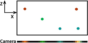
Figure 3. Image formation model illustration. Particles in different depths will be illuminated by different colors, leading to a corresponding camera response on the sensor (various point spread functions (PSFs)). The response of overlapped particles will be mixed.
Download figure:
Standard image High-resolution imageIntroducing regularization terms and constructing a minimization problem are common strategies to tackle this kind of problem. A sparse distribution of particles in the volume is expected, and the value of the particle distribution fields should be within the range of 0 and 1. These two constraints account for the second and third terms in line 2 of equation (1), where  is the L1 norm, and κ1 is the penalty parameter enforcing the sparsity. Here,
  denotes the weights compensating the sensor sensitivity to different wavelengths [25]; Π[0,1] is the operator projecting the value to the convex set [0, 1]. The fourth summation term in equation (1), referred to as the particle occupancy consistency, incorporates temporal coherence into the minimization problem, where
  indicates the advection of the particle distribution fields at time step t + 1 under flow field
  by −Δt units of time. Note that this term is also used for reconstructing velocity fields.
3.3. Velocity field () reconstruction

Having captured the particle fields in sequential time steps, we can then perform velocity estimation, in order to generate time-resolved velocity fields. A common method for such velocity estimation is Digital Volume Correlation (DVC), based on the cross-correlation of volume neighborhoods, or windows [14]. However, the selection of an appropriate window size can be difficult, since large windows result in overly smooth flow fields, while small windows can result in incorrect matches, particularly in the case of noisy, low-light images. Furthermore, such algorithms require a sufficiently high density of particles, which cannot always be satisfied for every flow scenario, especially in 3D measurements. Moreover, the cross-correlation based framework does not easily support adding extra physical constraints, such as divergence free flows in the case of incompressible fluids.
An alternative method is therefore adopted from the computer vision community, which solves the variational 'optical flow' problem (corresponding to 2D digital image correlation), by finding the correspondence between two successive particle distribution fields. The Horn-Schunck algorithm is the most widely used global variational optical flow method; this assumes a consistency of brightness between successive images, together with the smoothness of the flow vectors in the spatial domain. Here, instead of assuming the photo-consistency of 2D image intensities (the brightness consistency constraint does not hold, since the color of particles will change when they traverse different depth levels in axial direction), our 3D version of Horn-Schunck assumes a consistency of particle distribution fields  , as described in section 3.2. In this way, the particle occupancy consistency term ties particle and velocity reconstruction together into a joint optimization problem.
The framework described above is also amenable to the easy incorporation of the physical parameters of a given fluid. A number of works have already taken the physical constraints governed by Navier–Stokes equations into account when computing flows [6, 7, 16, 22, 26, 28]. In this work, we consider the fluids to be nonviscous and incompressible, which indicates zero divergence in the flow vectors. Moreover, the incompressible Navier–Stokes equation describes the time evolution of fluid flows. These two physical parameters account for the last two terms of equation (1). Here,  is the operation to project arbitrary flow vector fields onto a space having a divergence-free velocity field, where
  and
and  approximate the time evolution of the flow vector fields backward and forward, respectively. Note that we are not using the Navier–Stokes Equations to simulate flows; instead, we are incorporating them into the optimization problem as regularization terms.
A coarse-to-fine strategy is applied in our flow computation framework to solve large displacements. Roughly computed flow fields in the coarsest level are transmitted into finer levels as an initial guess, and are then iteratively updated, based on the fixed-point theorem (here, a pyramid of four levels and 10 inner iterations are applied). The algorithm stops when it reaches the finest level,where one vector per voxel is achieved.
3.4. Depth super-resolution
The depth resolution of the RainbowPIV system is dependent on the number of discretized depth levels, which is basically the number of PSFs. In our implementation, PSFs are expressed by a batch of 3 × 5 × 5 matrices, representing three color channels and a 5 × 5 spatial window. Owing to the relatively low sensitivity of the camera sensor to subtle wavelength shifts, only a limited number of PSFs is calibrated in the original RainbowPIV system, resulting in a relatively low depth resolution.
Specifically, the axial reconstruction accuracy relies on two factors: the camera's wavelength sensitivity, and the quantization error. The sparser the sampled signal, the larger the resulting quantization error. In this work, we show that it is feasible to reduce the quantization error by increasing the number of PSFs, using a simple linear interpolation scheme to generate in-between PSFs. As indicated in figure 4, in the prior implementation of RainbowPIV, the sampling rate in the axial direction is far lower than that in lateral directions, giving rise to a relatively large quantization error. With the proposed interpolation scheme, the same sampling rate can be achieved in all directions. While this change in PSF with wavelength is not linear over a large spectral range, piecewise linear approximations such as ours provide a good model of the true intensity change in each RGB color channel (see figure 5) over small spectral bands. With this simple digital adaptation (no hardware adjustment is required), we are able to generate super-depth particle distribution fields and flow vectors with reduced axial quantization errors. A similar interpolation scheme is also applied to reconstruct subpixel flow vectors between two images [8].
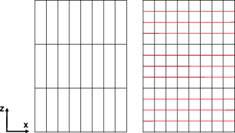
Figure 4. Discretization scheme for the precedent RainbowPIV (left) and the proposed strategy (right).
Download figure:
Standard image High-resolution image
Figure 5. Calibrated curves for the normalized camera response to different depth levels (0 - 25 mm) for red, green and blue channels. Spectral responses to 20 depth levels are obtained from calibration, and the curves are generated by linear fitting. These curves match well with the camera's spectral sensitivity curve with respect to wavelengths. Within a small spectral band, linear curve fitting is a simple, yet effective model for approximating camera response.
Download figure:
Standard image High-resolution imageWe now assess the effectiveness of this interpolation scheme on simulated data. Here, we simulate a volume with a fixed lateral dimension of 20 mm × 20 mm, and various axial dimensions (2 mm, 4 mm, 8 mm, 16 mm), yielding different depth-to-width ratios. We use the calibrated PSFs to model the camera's response to different depth levels. The lateral dimension is discretized by a size of 200 × 200, yielding a spacing of 0.1 mm. A random particle distribution of ppp = 0.05 is generated, and is advected following simulated flow velocities, as described in [26]. We compare the reconstruction errors of the flow vectors in the axial direction (referring to  ) for both standard RainbowPIV and the proposed depth super-resolved RainbowPIV. The results are shown in figure 6. When the depth-to-width ratio is 0.1, RainbowPIV and the new proposed approach are identical, as they have the same axial spacing. When the depth-to-width ratio increases, RainbowPIV samples the volume more sparsely in the axial direction, yielding increased axial reconstruction errors (almost linear to the depth-to-width ratio). Using the interpolated scheme, the axial reconstruction accuracy is significantly improved, based on the simulated results; errorsare reduced by roughly half when the depth-to-width ratio reaches 0.8. The accuracy of the reconstructed flow vectors using this approach is further experimentally validated below.
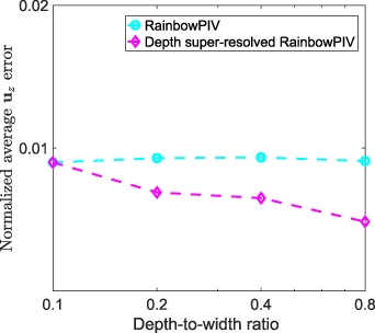
Figure 6. Averaged errors for reconstructed flow velocities in the axial direction with respect to various depth-to-width ratios. The error is normalized by dividing the volume depth.
Download figure:
Standard image High-resolution image4. Experimental results
4.1. Validation experiments
Here, we validate the proposed strategy using experimental data, including information relating to ground truth motion, based on the approach in [26]. We immerse the particles into a tank containing high viscosity liquid to "freeze" them. The tank is then put on a multi-dimensional rotation/translation stage. The true movement of particles can thus be managed by manipulating the stage. We move the tank in x and z directions, respectively, so as to compare the accuracy of both lateral and longitudinal reconstruction . A translation of 0.2 mm in the x direction and 0.5 mm in the z direction is applied. As a result, the standard RainbowPIV implementation [26] recovers a motion vector of 0.18 mm/time units, the mean value of the norm of the reconstructed velocity in the lateral translation, with a standard deviation of 0.015 (mm/time unit), and the proposed method delivers a similar reconstruction accuracy, 0.18 mm/time unit with standard deviation of 0.014 (mm/time unit). With regard to the longitudinal translation, 0.35 mm/time unit, with a standard deviation of 0.079 (mm/time unit) is achieved by the original RainbowPIV, while our super-resolved approach achieves 0.42 mm/time unit with a standard deviation of 0.045 (mm/time unit). We therefore observe a significant improvement with respect to axial reconstruction accuracy in this simple scenario, while the lateral reconstruction accuracy is unaffected.
In both implementations, the recovered lateral flows exhibit greater accuracy than the axial flows. As explained in section 3.4, quantization errors and camera wavelength sensitivity both affect the axial resolution. In the case of the original RainbowPIV, the sampling rate along the axial direction is lower than the lateral sampling rate, resulting in larger quantization errors. The super-resolved approach, in contrast, achieves an identical sampling rate in lateral and axial directions; however, the camera is more sensitive to lateral particle motions (changes in pixel positions) than axial motions (changes in wavelength). This fact brings in a great degree of uncertainty in relation to the estimation of axial flows.
4.2. RainbowPIV and Tomo-PIV
We further validate our method by directly comparing it with a four-camera Tomo-PIV system in relation to practical fluid flow phenomena. The simultaneous experimental setup for four-camera Tomo-PIV and single-camera RainbowPIV is shown in figure 7. The effective resolution of the captured RainbowPIV images is 1600 × 1120 (pixels). We downsample the images by a factor of 8 in both dimensions (no further image preprocessing required), resulting in 200 × 140 (pixels) images, and each particle occupies roughly 3 × 3 pixels. The depth dimension is discretized into 100 levels in order to obtain regular voxels, where the PSFs of 20 levels (1.25 mm per level) are obtained by calibration, and the intermediate PSFs are digitally generated by linear interpolation, based on the calibrated neighbor PSFs. Therefore, the size of the reconstruction grid is 200 × 140 × 100, with a voxel spacing of 0.25 mm along all three axes. One vector per voxel will be generated by the proposed algorithm; therefore, the reconstructed velocity field has the same dimensional size and spatial resolution as the grids (200 × 140 × 100). The particle image density is roughly 0.05 ppp (particles per pixel), and one example of the captured RainbowPIV image at this particle density is shown in figure 8. A qualitative comparison of the reconstructed velocity fields for the introduced vortex ring at one time step is presented in figure 9. Two sliced views (one perpendicular and the other parallel to the image plane) of the reconstructed flow vectors and the color-coded vorticity magnitude are visualized. The overall flow structure obtained by RainbowPIV agrees well with that computed by Tomo-PIV. Nevertheless, with its multiple perspectives, Tomo-PIV demonstrates greater depth resolving capability than the proposed single view approach. We can observe that the reconstructed flow vectors from RainbowPIV with a large z component are noisier than flow vectors in the x − y plane. As discussed in section 3.4, this is due to the relatively lower sensitivity of the camera to the wavelength change, so that the camera is less sensitive to particle motions in the axial direction than to in-plane motions. Quantitative comparisons between Tomo-PIV and RainbowPIV show an average difference of about 0.05 m s−1 for flow vector components in the x − y plane, and 0.1 m s−1 for vector components in the z direction, with a maximum flow magnitude of 0.53 m s−1. In comparison, the original RainbowPIV implementation has the same in-plane average difference, whereas the out-of plane difference is 0.21 m s−1. Although the uncertainty of the axial flow vectors is still larger than for the lateral flow vectors, these results affirm the improved axial resolution.

Figure 7. Experimental setup for both Tomo-PIV and RainbowPIV.
Download figure:
Standard image High-resolution image
Figure 8. A single captured RainbowPIV image with ppp = 0.05. Note that with the employment of the specifically designed diffractive optical element, different colored particles share a similar level of focus with the maximum aperture (f/1.8), even though they have different object distances.
Download figure:
Standard image High-resolution image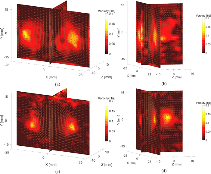
Figure 9. (a)–(b): Reconstructed flow vectors and vorticity magnitudes using RainbowPIV (the vector fields are shown every other 4 vectors for visualization purposes). (c)–(d): Reconstructed flow vectors and vorticity magnitude using Tomo-PIV. This simultaneous measurement is conducted at ppp = 0.05. The length of the arrow indicates the magnitude of the flow vectors. All the plots are in the same length scale.
Download figure:
Standard image High-resolution imageAn additional comparison is conducted by visualizing the isosurface of the vorticity magnitude, as shown at the top of figure 10. The figures reveal the similarity of the core structures reconstructed by these two measurement technologies. We further verify the mass conservation properties of the reconstructed flow fields, which should comply with their physical properties. The divergence of the computed flows is shown in the bottom of figure 10. Zero divergence is expected everywhere for incompressible fluids. This divergence-free property is explicitly enforced by our reconstruction method, whereas Tomo-PIV fails to generate flow fields obeying this physical property, and in addition does not readily support the addition of this constraint during computation. This result demonstrates that, despite the overall high quality and detail of the Tomo-PIV solution, it can in fact not be considered as a ground-truth solution.
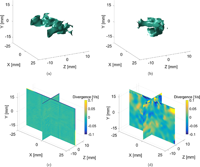
Figure 10. Isosurface visualization for the vorticity magnitude computed from RainbowPIV (a) and Tomo-PIV (b) at ppp = 0.05; The divergence of the velocity fields ( ) by RainbowPIV (c) and Tomo-PIV (d).
Download figure:
Standard image High-resolution image4.3. Low particle seeding density
Next, we evaluate the RainbowPIV system in low particle density situations, which are far below the desired particle density required by Tomo-PIV. The correlation-based algorithms applied in Tomo-PIV require sufficiently dense seeding particles to extract accurate flow fields, and usually perform poorly at low particle densities. The variant of the optical flow method presented here, however, ameliorates this issue by exploiting a local constraint (particle occupancy consistency), which ensures that in those regions where particles are present, the reconstructed local flow vectors match with the practical particle motion, and two global constraints (global smoothness constraint and temporal coherence), transmitting the accurate local flow vectors to those regions where particles are not present. Moreover, the physical properties are always satisfied, regardless of the particle density.
The tested particle image densities are roughly calculated as 0.005 and 0.015 ppp, and the captured images for these are shown in figure 12. The reconstructed flow vectors and vorticity magnitude are also visualized in figure 11, which demonstrates that RainbowPIV successfully captures the expected flow structures for vortex rings at various low density levels. Owing to its use of both local and global constraints, the proposed method delivers decent results at rather low particle densities. Under such conditions, particle tracking systems would be preferable to Tomo-PIV. However, this generates Lagrangian flow vectors with sparse descriptors, rather than the desired Eulerian vector fields. As a result, we believe that RainbowPIV can also be very competitive in experiments where uniform particle seeding is difficult or impossible.

Figure 11. Reconstructed flow vectors and vorticity magnitude from RainbowPIV at ppp = 0.015 (a)–(b) and ppp = 0.005 (c)–(d).
Download figure:
Standard image High-resolution image
Figure 12. Captured RainbowPIV images, where ppp = 0.015 (a) and ppp = 0.005 (b), respectively.
Download figure:
Standard image High-resolution image
5. Discussions
Depending on the setup, there are a number of possible alternatives for illumination, including high power white LEDs, or even super-continuum lasers. The volume size will determine the total light output required, but also the amount of spatial coherence or beam divergence of the rainbow. This then determines the choice of light source.
Currently, the reconstruction algorithm assumes a single exposure per video frame. Pulsed illumination at one pulse per frame could be used to suppress motion blur, without any changes to the software. However, multiple exposures per frame would require changes to the reconstruction; this may be a fruitful avenue for future research.
The maximum flow velocity retrieved by our technique is constrained by two factors: from the algorithmic perspective, the maximum flow vectors which can reliably be generated are 8 voxels (0.24 m s−1) between consecutive time steps (a coarse-to-fine strategy is applied to tackle the issue of large displacements). From the image quality perspective, like all other PIV measurement systems, fast-moving particles (along the lateral directions) cause severe motion blur in the captured images, which downgrades the reconstruction accuracy.
As indicated in figure 5, the sensitivity of the color-based depth-encoding scheme is non-uniform along the depth axis. However, we did not observe correlations between the flow reconstruction accuracy and depth-encoding sensitivity. The main reason for this is that our flow estimation framework is composed of both local and global constraints (elaborated in section 4.3). The sensitivity of the depth-encoding scheme only accounts for the local constraint, and the reconstructed flows are also managed by the other global constraints.
6. Conclusion
In this article, we have proposed a depth super-resolved RainbowPIV system which overcomes the limitations of axial resolution inherent in the precedent RainbowPIV system. A comprehensive study has been conducted to compare RainbowPIV with the well developed four-camera Tomo-PIV approach, using a simultaneous measurement setup. Both qualitative and quantitative results demonstrate the good agreement achieved by these two systems. In addition to velocity consistency, due to the physically-constrained velocity estimation model, RainbowPIV delivers divergence-free velocity fields for the measured incompressible fluids, whereas Tomo-PIV fails. Moreover, with the employment of both local and global constraints, RainbowPIV successfully reconstructs velocity fields at rather low particle densities, which is restricted using Tomo-PIV. All the observations confirm the potential application of RainbowPIV in 3D volumetric velocity measurements, particularly in applications with limited optical access and low or non-uniform particle densities.
Acknowledgment
This work was supported by the King Abdullah University of Science and Technology, via the CRG grant program, as well as individual baseline funding.