
Abstract
We propose a new frustrated Heisenberg antiferromagnetic model with spatially anisotropic exchange parameters Jc, Ja, and Jac, extending along the c, a, and a ± c (c–a–ca model) lattice directions, and apply it to describe the fascinating physics of copper carbodiimide, CuNCN, assuming the resonating valence bond (RVB) type of its phases. This explains within a unified picture the intriguing absence of magnetic order in CuNCN. We further present a parameters–temperature phase diagram of the c–a–ca-RVB model in the high-temperature approximation. Eight different phases including Curie and Pauli paramagnets (respectively, in disordered and 1D- or Q1D-RVB phases) and (pseudo)gapped (quasi-Arrhenius) paramagnets (2D-RVB phases) are possible. By adding magnetostriction and elastic terms to the model, we derive possible structural manifestations of RVB phase transitions. Assuming a sequence of RVB phase transitions to occur in CuNCN with decreasing temperature, several anomalies observed in the temperature course of the lattice constants are explained.
Export citation and abstract BibTeX RIS
1. Introduction
Among the materials of the MNCN series (M =Mn, Fe, Co, Ni), the phase CuNCN is the most peculiar example [1]. In variance with other members of the series exhibiting more or less standard antiferromagnetic behavior, CuNCN is a temperature independent (quasi-Pauli, see below) paramagnet at room temperature and, at lower temperatures, switches to a gapped (quasi-Arrhenius) temperature dependence. Nonetheless, it is not metallic in the temperature range where the Pauli paramagnetism occurs, hence no metal–insulator transition can be responsible for the quasi-Arrhenius behavior. It also does not manifest any magnetic neutron scattering [2] so that no long-range magnetically ordered (LRMO) state appears to which one could ascribe the susceptibility drop. These findings brought us [3–6] to the idea that CuNCN may form resonating valence bond (RVB) phases of the Cu2+ local spin 1/2 which are unequivocally observed in the Pauli paramagnetic phase with use of EPR [4]. This idea allowed us [3–6] to explain the magnetic and polarized neutron experiments by further assuming that the RVB phases are those of an anisotropic triangular antiferromagnetic Heisenberg model evolving in the ab crystallographic plane (figure 1). Can one expect structural manifestations of the conjectured transition between the RVB phases? Yes, because instead of the typical decrease of the unit cell dimensions one detects an anomalous temperature dependence of the lattice parameter a in synchrotron experiments, to be related with the 1D-RVB to 2D-RVB phase transition of the anisotropic triangular Heisenberg model which opens the gap in the quasiparticle spectrum along the a direction [5, 6].
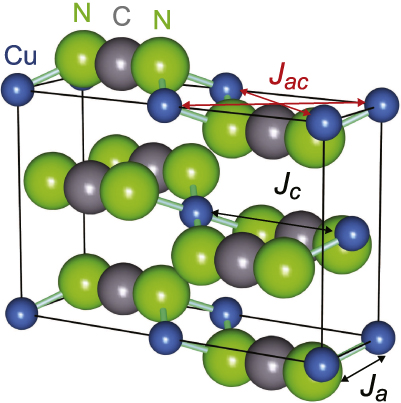
Figure 1. Crystal structure (unit cell) of CuNCN and exchange parameters included in the consideration. Those in the ac crystallographic plane are taken into consideration. The interactions are always mediated by the NCN2− moieties. Two stronger interactions (Jc and Jac) are mediated by the π-system of NCN2− and extend, respectively, in the c and c ± a directions; they in fact couple the Cu2+ ions shifted by one half of the lattice parameter in the c direction; somewhat weaker Ja contributed by a ferromagnetic counterpoise term dependent on the hybridization at the N atoms extends in the a direction.
Download figure:
Standard image High-resolution imagePuzzlingly, the experiment [6] also shows some irregularities for the lattice parameter c at about the same temperature (80–100 K) as for the lattice parameter a, and there are more irregularities in either the a- or the c-direction at about 30 K (see figure 2).
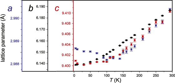
Figure 2. Course of the lattice parameters a,b, and c of CuNCN as a function of the temperature (see [6] where the experimental details can be found). Data for the first run (λ = 0.501 95 Å) are given by squares and those for the second run (λ = 0.503 50 Å) by bullets. One can see that the temperature course of the b parameter (black) shows no anomaly, whereas both the a and the c parameter (respectively, blue and red) go in opposite directions below 100 K and exhibit other anomalies at about 30 K.
Download figure:
Standard image High-resolution imageThe hypothesis of the triangular lattice is also not easy to reconcile with the intuitive picture [7] of the most important couplings extending along a and c. This brings us to the idea of considering more antiferromagnetic couplings and of formulating the Heisenberg model with the Hamiltonian

where the translation vector τ takes four values τi,i = 1–4: τ1 = (a,0);τ2 = (0,c);τ3 = (a,c);τ4 = (a, − c), with an interaction of strength Ja along the lattice vector τ1 (two neighbors), an interaction of strength Jc along the lattice vector τ2 (two neighbors as well), and an interaction of strength Jac along the lattice vectors τ3 and τ4 (two neighbors along each)—see figure 1. Either interactions along τ1 and τ2 or those along τ3 and τ4 taken separately must lead to an antiferromagnetic state. However, when considered simultaneously they interfere leading to a frustration not allowing the spins to arrange in any LRMO state. For similar systems a variety of RVB states have been proposed [8, 9]. Ground states of a similar, but spatially isotropic J1J2J3 model have been treated recently by various methods, and it has been shown that spin-liquid (RVB) states are very probable [10]. This generalizes the known Nersesyan–Tsvelik model [11] which derives from ours by setting Ja = Jc, which is clearly not the case for CuNCN. In this paper, we consider in detail the RVB states of the above model in the mean-field approximation and apply this approximation to analyze the experimental data so far obtained for CuNCN.
2. RVB mean-field analysis of the model
2.1. Quasiparticle spectrum
Following the method [12] we use the fermion (spinon) representation of the spins,

where  are the fermion creation (annihilation) operators; σαβ are the elements of the Pauli matrices and summation over repeating indices is assumed. Applying the technique as described in appendix A (this method widely applies to various layered cuprates and is a standard treatment) we arrive at the quasiparticle spectrum,

where we set x = kx,z = kz and introduce effective order parameters (OPs) ζa,ζc, and ζac describing the states of the model.
The spectrum (3) is depicted in figure 3. It shows three principal regimes: (i) one with two pairs of lines of nodes (gapless 2D-RVB), (ii) one with a pair of lines of nodes (termed as 1D- and Q1D-RVB states), and (iii) one with two pseudogaps and four nodal points (pseudogapped 2D-RVB)—for the naming of the states see below.

Figure 3. Dispersion laws (quasiparticle energy—applicata, versus 2D-wavevector in the Brillouin zone k∈[ − π,π] × [ − π,π]—abscissa and ordinate) of the c–a–ca-RVB model for several characteristic values of the OPs ζa,ζc, and ζac indicating key features of the quasiparticle spectrum in different RVB states and the sketches of the relevant qDoS—normalized number of states versus quasiparticle energy ε (see text for details).
Download figure:
Standard image High-resolution imageIf either of the OPs ζa or ζc is the only nonvanishing OP, the quasiparticle spectrum acquires corresponding lines of nodes  (or
(or  ) where the quasiparticles have zero energy. We call these states one-dimensional (1D-RVB) states since the dispersion of quasiparticles occurs in only one crystallographic direction (a or c—see, however, below). The quasiparticle density of states (qDoS) in the 1D-RVB states is constant at zero energy, but it diverges at the ceiling of the quasiparticle band due to the dispersionless ridge in the spectrum [3], similarly to the 1D-RVB state of the anisotropic triangular Heisenberg model found in [13]. If both OPs ζa,c vanish and the OP ζac does not, two pairs of nodal lines exist along which the quasiparticles have zero energy. In this state the qDoS diverges logarithmically at zero energy.
If either of the nonvanishing OPs ζa,c is complemented by the nonvanishing OP ζac, quasi-1D-RVB (Q1D-RVB) states appear. The difference from the true 1D-RVB states is that in the Q1D-RVB states one finds a nonvanishing dispersion transverse to the node lines, so that the quasiparticle spectra have local maxima and saddle points instead of a ridge. Thus, the qDoS develops a finite hop at the ceiling of the quasiparticle band and a logarithmic singularity at the pseudogap. By contrast, if the nonvanishing OPs are ζc and ζa, then (irrespective of the OP ζac) there are no lines of nodes, but four nodal points ( ) of vanishing quasiparticle energies. The two possible states of this type are called 2D-RVB. The qDoS in 2D-RVB states vanishes at zero energy, being proportional to the energy well below the smaller pseudogap. Otherwise the quasiparticle dispersion law has saddle points at the two pseudogap energies and, thus, the qDoS of the 2D-RVB state develops two logarithmic singularities at the corresponding pseudogaps. In the Nersesyan–Tsvelik model (Ja = Jc) two logarithmic peaks coalesce and only one pseudogap is manifested. The exact forms of the qDoS of all RVB phases of the model are given in table C.1, appendix C. In the last column of table C.1 we show the analytical forms of the qDoS characteristic for the respective forms of the quasiparticle spectrum. It turned out quite unexpectedly that these qDoS can be found analytically for all phases of the c–a–ca-RVB model. Leaving the details of the derivation for a further publication we provide its sketch in appendix C.
2.2. Free energy and phase diagram of the model
The thermal behavior of the c–a–ca model derives from its free energy which can be written immediately [9] as
where θ = kBT and BZ stands for integration over the Brillouin zone. The minima of the free energy (4) with respect to the ζs correspond to possible phases of the system. The study of the ground state (zero-temperature limit) of the present model will be published elsewhere [14]. Here we focus on the results which can be obtained with use of the high-temperature expansion (technicalities are explained in appendix B). Minimizing the high-temperature expansion of (4) with respect to the OPs, we obtain the parameter phase diagram shown in figure 4 for the triple of the reduced exchange parameters subject to the condition  and a series of reduced temperatures θ* between 0.4 and 0.01 (the fractions of the above sum of the reduced exchange parameters are meant). Eight phases are possible. For the temperature above either of three critical ones,

the 'gray' phase persists in which all three OPs are equal to zero.
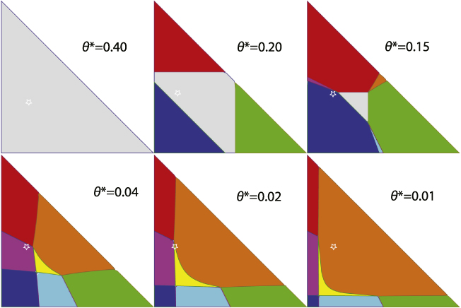
Figure 4. Parameter phase diagrams for the c–a–ca-RVB model in the high-temperature approximation. The abscissa and ordinate represent the reduced parameters  and
and  ; these parameters, respectively, are equal to unity in the lower right and upper left corners; the entire set of reduced parameters is subject to the condition
  . The reduced temperatures θ* are fractions of
  . The color coding for phases is as follows: Curie paramagnetic, with all OPs zero =gray, only one nonvanishing OP =red or green (1D-RVB, Pauli paramagnet), = blue for ζc,ζa,ζac ≠ 0, respectively; one OP vanishing= magenta, cyan (Q1D-RVB, Pauli paramagnet), =orange for ζa, or ζc, or ζac = 0, respectively—observe the order of the list; yellow codes the phase with three nonvanishing OPs. Orange and yellow phases (2D-RVB) feature a combination of the gapped Arrhenius-like temperature dependence of magnetic susceptibility and its linear dependence well below the pseudogap. The small star shows the tentative position of CuNCN on the parameter phase diagram.
Download figure:
Standard image High-resolution imageBelow these temperatures, gapless phases appear in respective corners of the parameter phase diagram. There are two 1D-RVB phases with OPs ζc or ζa ≠ 0 (red and green areas in figure 4). The gapless 2D-RVB phase with only one OP ζac ≠ 0 occupies the blue area in figure 4.
Below the critical temperatures

the corresponding phases with two nonvanishing OPs ζτ and ζτ' appear (the notation refers to a transition from the state with one nonvanishing OP, ζτ ≠ 0, to a state with two nonvanishing OPs, ζτ,ζτ' ≠ 0). The phases with two nonvanishing OPs are different as well. If one of the nonvanishing OPs is ζac (magenta and cyan areas in figure 4) these are Q1D-RVB phases. If the two nonvanishing OPs are ζc and ζa, a 2D-RVB phase (orange) appears from the 1D-RVB phases (red and green).
The phase with three nonvanishing OPs (yellow) can only appear below the octal point  where the phase with three vanishing OPs (gray) completely disappears and shows up from the above Q1D-RVB phases (magenta or cyan) at the critical temperatures

( for τ = a,c). It is transient and exists only above the critical temperature of

where it switches to the 2D-RVB phase with two nonvanishing OPs (orange). The only difference between the dispersion laws in these two 2D-RVB phases is somewhat more pronounced dispersion along a 'ridge' in the case of the phase with three nonvanishing OPs. Otherwise both pseudogapped 2D-RVB phases have a qDoS with two van Hove singularities at the energies of their characteristic pseudogaps, and their physics has to be pretty similar. All phase transitions are of second order, that is to say that the OPs split from zero continuously at the corresponding transition temperatures. Obviously, in the high-temperature approximation only the classical value of the critical exponent  can appear.
In general, one can expect that the high-temperature expansion will be valid down to temperatures of the order of J. This is, however, a too conservative estimate. It had been shown in [9] that the high-temperature estimate for the critical temperature of the transition between the Curie and Pauli paramagnetic phases of the anisotropic triangular Heisenberg model, which coincides with (5), precisely reproduces the numerical result, showing by this that the high-temperature expansion in a frustrated system remains valid for temperatures reasonably below 0.5J. Furthermore, the lower critical temperature given by (6) as well is in fair agreement with the numerical result of [12] for the anisotropic triangular Heisenberg model as shown in [3, 5]. This shows that the validity range of the high-temperature expansion in fact extends down to about 0.1J', where J' < J is a smaller (oblique) exchange parameter of the anisotropic triangular Heisenberg model. Thus at least in the most studied frustrated model the number and approximate positions of critical points are semiquantitatively reproduced by the high-temperature expansion which in that sense remains valid down to a pretty low temperature. This turns out to be true for a frustrated system—where the motions remain chaotic due to the frustration. That is why we cautiously rely on this method for our new frustrated Hamiltonian.
In order to make the not particularly intuitively clear minima of the free energy (4) more comprehensible we on the basis of the analysis of [9] represent pictorially the characteristic microstates contributing to the respective phases in figure 5. According to [9] the RVB wavefunction is a superposition (linear combination/resonance) of microstates written with respect to individual spins residing in the vertices of a lattice. In the case of the c–a–ca model these are the vertices of a rectangular lattice with the constants a (horizontal in figure 5) and c (vertical in figure 5). In the microstates all spins form singlet pairs (valence bonds) of the form  . The microstates are thus the products of valence bonds for different pairs of vertices rr' such that in a given microstate each spin enters in one and only one valence bond. Being summed with different amplitudes controlled in their turn by the values of the OPs symbolized by the ⊕ sign, the microstates produce specific RVB states. The states with a single nonvanishing OP are easiest to understand. These are the gapless 2D- and 1D-RVB states shown in two leftmost panels of figure 5. In these states the bonds appear only along the directions where the OPs are nonvanishing. Thus the 1D-RVB states differ, as one can imagine, by the directions (a or c) in which the bonds extend. Formally, being directed in, say, the c direction means that for all bonds the following holds: r = r' + nc, with an integer n, and analogously for the 1D-RVB state extended in the a direction. We use the color code of the respective phases in figure 4 to render the bonds extended in the corresponding directions. In the Q1D-RVB states the bonds extended in one of the lattice directions are complemented by those coupling the spins along the geometric diagonals: a ± c. In the (pseudo)gapped 2D-RVB states the bonds extend in either direction along the crystallographic axes. The 2D-RVB state with all three nonvanishing OPs (yellow) contains all possible bonds, whereas the 2D-RVB state with vanishing ζac (orange) misses the bonds extended along the geometric diagonals, as can be seen in the two rightmost panels. The above considerations apply to the pure RVB states, i.e. at zero temperature. For the respective RVB phases at finite temperature the depicted ground states of each type are accompanied by excited states taken with respective statistical weights, in which some temperature dependent fraction part of the bonds is broken.

Figure 5. Characteristic spin-pairing (valence bond) contributing to produce various RVB states. See text for details.
Download figure:
Standard image High-resolution image3. Physical properties of CuNCN viewed through the model
As mentioned above and previously [3–5], the absence of magnetic scattering in CuNCN is perfectly explained by the hypothesis of the RVB character of its phases. The magnetic properties (qualitative behavior of the susceptibility as a function of temperature) as deriving from the characteristic features of the qDoS are designated in the first column of table C.1. It is not surprising that the temperature-independent paramagnetism (conditionally denoted as 'Pauli', although it goes about spinons rather than conductivity electrons) occurs in the (Q)1D-RVB phases with a constant qDoS at zero energy. The 'blue' gapless 2D-RVB phase with two pairs of intersecting node lines is manifested as a logarithmic singularity in the qDoS at zero energy. This singularity integrates and produces a logarithmic divergence of the susceptibility at zero temperature which qualitatively would be difficult to distinguish from the Curie paramagnetism. For two pseudogapped 2D-RVB phases (yellow and orange) with nodal points in the dispersion law and linear dependence of the qDoS in the low-energy range one has also to expect a linear temperature dependence of the susceptibility in the low-temperature region (well below the smaller pseudogap) superimposed with a quasi-Arrhenius behavior with characteristic energy of the pseudogap at higher temperature. This rich variety of possible phases in the c–a–ca-RVB model allows us to eventually explain the magnetic behavior of CuNCN. As previously, we assume that the (Q)1D-RVB phase sets in at some fairly high temperature which cannot be directly checked due to decomposition of the material [4]. Incidentally, Curie paramagnetism is not observed in CuNCN in the range of its thermal stability. The same applies to the gapless 2D-RVB phase with logarithmically divergent susceptibility. The Pauli paramagnetism, which changes to the quasi-Arrhenius gapped regime, is thus logically attributable to the (Q)1D-RVB phases, transforming to the pseudogapped 2D-RVB phases at lower temperatures. By this, the entire picture of the magnetic properties of CuNCN is qualitatively reproduced.
The observed magnetic behavior qualitatively reconciles with the temperature course of the lattice parameters a and c (figure 2). The sequence of the parameter phase diagrams shows which specific RVB phases emerge at the specified temperatures in the respective areas of the parameter space. The CuNCN species is characterized by a specific set of parameter values derived in appendix D (see also below), mapping to one point in the parameter space marked by the star. At different temperatures various phases occupy slightly different areas of the parameter space. In the lower row of figure 4 we can see how the point representing CuNCN while staying in its original place effectively moves from one phase to another: subsequently changing from the Q1D-RVB (magenta) to the transient 2D-RVB (yellow) and finally to the low-temperature 2D-RVB (orange).
Below the octal point θ* = 1/8 (the lower row of ternary diagrams in figure 4), the thermal evolution consists en gros in squeezing out all the phases by the 2D-RVB phase with vanishing ζac (orange). The 2D-RVB phase with three nonvanishing OPs (yellow) is transient, so its parameter area is never large and it is subject to deformations and displacements under the 'pressure' of the orange phase. The parameter estimate of appendix D positions CuNCN on the parameter phase diagram (figure 4) at the point with the reduced parameters (barycentric coordinates)  , i.e., within the magenta phase, but close to and somewhat below the quadruple point of the red, magenta, orange, and yellow phases in the leftmost graph in the lower row. In this row one can observe the following sequence of transitions between the RVB phases:
upon decreasing temperature. The thermal dependence of the OPs within these phases is described by the expressions given in table 1. One should not expect that these expressions derived from the high-temperature expansion for the free energy will be exactly valid at low temperature. Specifically, the prefactors θ should not be taken seriously since it has been shown [14] that the exact ζa,c OPs flow to some finite values as the temperature flows to zero. Thus, the OPs split from zero values at the critical temperatures given next to them. Since the exchange parameters satisfy the condition Jac⪆Jc, the OP ζac is always small and decreases with decreasing temperature, thus we do not consider it explicitly further. The OP ζc increases either in the magenta or in the yellow phase according to the same law (the reference/critical temperatures for this OP in these two phases are equal), but we assume that in the interesting temperature range  it has almost reached its zero-temperature limit and does not significantly change any more1. The OP ζa splits from zero at the critical temperature of
  (transition to the yellow phase). Finally, at the lowest accessible critical temperature
  (8) a transition to the orange phase takes place2. The transition to the orange phase (evanescence of ζac) at
  whatever it is affects neither the bandwidth, since this OP is never large, nor the character of the temperature dependence of ζa, although some variation of its slope can be expected. At this phase transition, however, a remarkable change can be expected in the character of the temperature dependence of ζc. Namely, it switches from an increase to a decrease when the temperature decreases. This happens because of an instantaneous change of its reference temperature shown in table 1 from positive
  in the yellow phase to
  in the orange phase, which is negative in the relevant area (Jac⪆Jc > Ja) of the exchange parameter space. Changing the sign of the reference temperature causes the change of the temperature course of the OP ζc which, in the orange phase, starts to decrease with temperature decrease instead of being constant (or very slowly growing) in the yellow phase.
Table 1. Temperature dependences of the OPs for possible phases of CuNCN in the high-temperature approximation of the c–a–ca-RVB model. The areas of existence of the corresponding phases are given by the condition of positiveness of the expressions under the square roots.
| Color code | OPs versus θ |
|---|---|
| Blue |
|
| Magenta |

|
| Yellow |

|
| Orange |

|
Previously [5, 6], we were able to explain the temperature anomaly of the a lattice parameter by attributing it to opening a gap in the quasiparticle spectrum in the crystallographic direction a and formation of a gapped 2D-RVB state in the triangular anisotropic Heisenberg model. This is accompanied by the split of an RVB OP from zero, which is coupled to the lattice constant through 'magnetostriction' terms. Although the previous model (triangular anisotropic Heisenberg lattice) could not be fully substantiated, similar moves absolutely apply in the present model with three exchange parameters and respective OPs. We assume as previously a linear relationship between the exchange parameters Jτ and geometry parameters ρλ,

Following [15] we assume that zero values of ρs correspond to a hypothetical structure, which the CuNCN crystal would have provided the exchange interactions Jτ were turned off. The observed geometry of the crystal where the exchange interactions result in the formation of one of the RVB phases corresponds to the minimum with respect to ρλ of the free energy (4) to which the elastic energy (E.1) is added, and the exchange parameters are replaced according to the recipe (10). Using the special form of the RVB free energy (4) we arrive at the explicit expression (for details see appendix E)
the sought relation between the RVB OPs and their structure manifestations (Aτ are the numerical coefficients: 3 for τ = a,c; 6 for τ = ac) which further generalizes the famous bond-length–bond-order relation to the RVB states.
The temperature dependence of the structure described by the parameters ρλ is thus that of the relevant combination of the squares of the corresponding OPs. In the magenta and yellow phases the OP ζc is (almost) temperature independent, thus  does not contribute to the visible variation of the lattice constants; therefore we focus first on the contribution of the OP ζa (our previous consideration allows us to neglect the OP ζac).
Before switching to rationalizing the low-temperature behavior of the lattice parameters shown in more detail in figure 6, we stress once again that our purpose is to provide a unified view of the data obtained in polarized neutron scattering [2], susceptibility [1, 4], and structure (synchrotron [6] and neutron [16]) experiments. Thus, in our reasoning we follow the above unifying concept in the hope that minor inconsistencies (possibly coming from the uncertainty in the measurements or sample irregularities) can be resolved in the future. In order to proceed we introduce geometry variables ρa = δa = (a − a0), 2ρc = δc = (c − c0), and assume that the exchange constant Ja is independent of the deformation in the c-direction (see below). Thus,  , and we apply the general relation (11). In this setting the variation of two lattice parameters is
where |K| is the determinant of the 2 × 2 matrix of the force constants. Clearly, the off-diagonal force constant Kac makes the lattice parameter c sensitive to variations of the OP ζa. Moreover, the effect on c is predicted to have the opposite sign to that on a (a increases, c decreases, and vice versa). When the pseudogap opens in the a direction (about 100 K), two lattice parameters have to start changing in opposite directions, as observed. The same behavior can be traced in the neutron scattering data [16] which are going to be analyzed in detail in a forthcoming publication.

Figure 6. The temperature dependence of the lattice parameters in the low-temperature range as extracted from synchrotron diffraction data [6] (red dashes with error bars). (a) The temperature course of the a lattice parameter. The linear models with the slopes −7 × 10⁻⁶ Å K−1 (in the 2D-RVB phase with three nonvanishing OPs—green line) and −5 × 10⁻⁶ Å K−1 (in the 2D-RVB phase with two nonvanishing OPs—blue line). (b) The temperature course of the c lattice parameter. The linear models here are largely guides to the eye, but the corresponding slopes are −13 × 10−6 Å K−1 (blue line) and 17 × 10−6 Å K−1 (green line).
Download figure:
Standard image High-resolution imageThe crucial point is the sign of the effect. At first glance the situation seems to be counterintuitive since in order to conform with the experimental increase of the a-parameter in the 2D-RVB phase with two pseudogaps (orange or yellow) as compared to the (Q)1D-RVB phase (red or magenta) the exchange parameter Ja has to increase with an increasing Cu–Cu interatomic separation. However, the effective value of the (antiferromagnetic) exchange parameter Ja is a sum of contributions of different signs,

where both Ja(antiferro) and Ja(ferro) are positive. The antiferromagnetic contribution is accumulated on numerous superexchange paths and is weakly affected by the Cu–Cu interatomic separation since no direct matrix elements between the states of the two Cu atoms affect Ja(antiferro) 3. By contrast, the ferromagnetic contribution strongly depends on the angle  (see [7, 17]), and in the range of
  , which is the case for CuNCN, decreases, while the
  angle and thus the Cu–Cu separation increases. Likewise, the overall effective antiferromagnetic exchange parameter Ja increases while the counterpoising ferromagnetic contribution decreases in absolute value. This explains the overall positive sign of
  and, thus, the experimental fact of increasing lattice parameter a in the phase with the pseudogap developing along the a-direction. Due the above sign relation between the effect of the a-pseudogap opening on the a- and c-lattice parameters, the experimentally observed extra decrease of the c lattice parameter at 100 K is explained as well.
The available data are insufficient to solve the subtle question of the critical exponents of the OPs. However, assuming the classical value of the critical exponent  prescribed by the high-temperature expansion as a plausible interpolation in a way confirmed by fitting the susceptibility run in the 2D-RVB phases (see appendix D), the lattice parameters must obey the linear temperature evolution, i.e., one with the exponent 2β. The latter is approximately observed for the lattice parameter a in a wide range below the (Q)1D- to 2D-RVB transition at about 100 K which, however, changes to a somewhat more chaotic behavior at about 30 K. It incidentally corroborates with the temperature course of the c lattice parameter measured in the synchrotron experiment [6] (figure 6(b)) which has not received due attention so far. As one can see, the lattice parameter c generally decreases with temperature. This behavior is in line with the usual thermal expansion and thus does not require any special explanation. It shows noticeable irregularities (not changing the sense of the course) at about 80–100 K, where the magnetic susceptibility changes from the quasi-Pauli to the quasi-Arrhenius regime, which has been explained above through its interplay with the opening of the pseudogap in the a-direction right in this temperature range. The sense of the temperature course of c changes at 30 K where the lattice parameter a starts to show irregularities in its turn. This, however, nicely fits in the above picture of the RVB phase transitions. Since the available amount of experimental data does not suffice to reliably estimate quite a few magnetostriction and other parameters required for the quantitative description, we try to derive a qualitative description in terms of the slopes of the lattice parameters versus temperature at critical points. In the minimal setting (i.e. neglecting the off-diagonal force constants and magnetostriction terms) we immediately obtain for the slope of c versus θ

At the transition from the yellow to the orange phase this slope has to change its sign since that of θcrit instantaneously changes from positive in the yellow to negative in the orange phase, as explained above, and that is precisely what happens. We also conclude that the magnetostriction parameter  has an intuitively understandable sign: it is negative since this exchange parameter is dominated by the electron transfers through the π-systems of the NCN2− units which in their turn strongly depend on the Cu–N interatomic separations affected by the deformation in the c-direction (see footnote 3). The temperature slope must therefore be negative in the orange (low-temperature) phase and positive in the yellow (transient) one, and that is again what happens.
In a more general setting the contribution of the OP ζc to the slopes of the lattice parameters versus temperature is
so that it is clear that the contribution of the variation of the OP ζc to the slope of a versus θ changes its sign when going from the yellow to the orange phase. The visible decrease of the negative slope of a in absolute value as seen below 30 K (in the orange phase as compared to the yellow phase) requires that the addition to it coming from ζc is positive. Semiquantitatively, this requires that  since in the orange phase θcrit in the above expression equals the negative
  . Incidentally, the term
  has the required sign as estimated above. Thus,
  has to be either positive, which is in principle conceivable as the above example of
  shows, or at least not too strongly negative. This tentatively explains the anomalies observed in figure 6.
4. Conclusion
A new form of the frustrated spatially anisotropic antiferromagnetic Heisenberg Hamiltonian close to the popular J1J2J3 model with exchange parameters Jc, Ja, and Jac extending along the c,a, and a ± c directions of a two-dimensional rectangular lattice is proposed. When applied to model the fascinating physics of copper carbodiimide (CuNCN) it explains the absence of magnetic order in CuNCN down to 4 K by assuming a resonating valence bond (RVB) character of its emerging phases. The quasiparticle spectrum of the RVB model of the proposed Hamiltonian shows three principal regimes: (i) a state with two pairs of lines of nodes, (ii) states with a pair of lines of nodes (termed as 1D- and Q1D-RVB states), and (iii) states with two pseudogaps and four nodal points (2D-RVB states). The extraordinarily rich parameters–temperature phase diagram of the model contains eight different phases whose magnetic behavior includes Curie and quasi-Pauli paramagnetism (1D- and Q1D-RVB phases), and (pseudo)gapped (quasi-Arrhenius) paramagnetism (2D-RVB phases). Both the quasi-Pauli and quasi-Arrhenius regimes are reliably observed in experiment. By adding magnetostriction and elastic terms to the free energy of the model, the temperature dependence of the CuNCN crystal structure is explained through a sequence of transitions between different RVB phases when the temperature decreases. Confronting the model with magnetic susceptibility and structure data recorded as functions of temperature between about 10 and 200 K, one finds remarkably good agreement between the theoretical predictions and the experiments.
Although structural manifestations are well known to accompany various magnetic transitions, e.g. [19], the specific result of this work is the unified description of the somewhat contradictory combination of absence of magnetic order, nongapped (Pauli) and gapped (Arrhenius) temperature courses of the magnetic susceptibility in the respective temperature ranges and structural effects coupled to the latter. The RVB hypothesis has a crucial importance not for the structural effects themselves, although we concentrate on them in this paper, but as an 'integrating factor' allowing us to explain from a unified viewpoint the facts coming from different experimental methods.
The spin-Peierls state in the c-direction could be a good ground state candidate within the picture of a strong exchange extended in this direction mediated by the NCN2− units. Had the spin-Peierls be there it would explain at least two key features of CuNCN: the activation dependence of the susceptibility due to opening of the spin-Peierls gap and the absence of magnetic long-range order visible in the neutron experiments due to the formation of alternating Cu–Cu spin pairings along the c-direction. Unfortunately, this intellectually attractive picture has to be abandoned for the time being since no signature of superstructure in either direction could be traced in the available structural data.
Acknowledgments
This work has been performed with the support of the DFG. Dr Andrej Zorko of Jožef Stefan Institute (Ljubljana, Slovenia) is acknowledged for sending numerical data on the ESR susceptibility [4]; Dr Wouter van Beek of Swiss–Norwegian Beamlines at ESRF and Professor Dr Uwe Ruschewitz of the Institute of Inorganic Chemistry, University of Cologne are acknowledged for sending the structure data of [6] in numerical form. The referees are acknowledged for instructive comments and suggestions.
Appendix A.: Equations of motion and self-consistency equations
The equations of motion are based on the Heisenberg representation in which each operator obeys

where [...,...] stands for the commutator and the ' ' for the time derivative. Applying this to the creation and annihilation operators
  and performing commutation, mean-field decoupling and Fourier transformation as done previously [3] results in their mean-field equations of motion,
The latter reduce to the set of 2 × 2 eigenvalue problems for each wavevector k,
with
The summation over τ extends to τi;i = 1–4, which results in the eigenvalues
whose eigenvectors are combinations of the annihilation and creation operators with the coefficients uk,vk. This set of equations is closed by the self-consistency conditions
for the order parameters (OPs). The lattice-symmetry considerations allow us to restrict ourselves to the OPs: ξa,ξc,ξac;Δa,Δc,Δac. For the complex OPs we introduce a polar representation,

The standard moves foreseen for the SU(2) symmetric solutions are used to exclude the cross terms in the OPs from  , which leads to the system of three equations

Introducing the relative phases as θa = φa − φac, θc = φc − φac, we arrive at equations of the form4
similar to those derived in [8] which can be satisfied, e.g., by setting
Of course, the OPs can also be vanishing.
Under the above conditions the spectrum of quasiparticles acquires the form

where we set x = kx;z = kz. Obviously, the solutions of the problem depend only on the effective OPs  ,
,  , and
, and  .
.
Appendix B.: High-temperature expansion
At high temperature we can use the expansion
which, when inserted in the formula (4), integrates explicitly. For determining the critical temperatures to the first approximation it suffices to restrict ourselves to the second-power terms. This results in an expression quadratic in ζτ. Combining the thus obtained 'kinetic' energy

with the potential energy terms from equation (4), we arrive at

This result can be improved with use of the Ginzburg–Landau approximate free energy FGL(ζτ,θ), which involves the terms up to the fourth power in ζτs. They appear from the integration of the fourth power of the spectrum which is performed explicitly and yields the 'kinetic' energy of the form
which together with the potential energy yields the free energy FGL(ζτ,θ) used for further analysis.
Appendix C.: Quasiparticle densities of states in various RVB phases
In section 2.2 we gave an impression of the complexity of the phase diagram of the RVB model with three exchange parameters. We also gave a brief description of the most characteristic features of the qDoS in various RVB phases. Here we provide a brief sketch of the derivation of the qDoS given in table C.1.
Table C.1. The qDoS in the possible phases of the c–a–ca-RVB model in the high-temperature approximation. Their characteristic graphs are given in figure 3. The pseudogap/bandwidth parameters in this table are A = 3Jaζa, C = 3Jcζc, B = 3Jacζac. In the last column K stands for the complete elliptic integral of the first kind. Details of the derivation will be communicated elsewhere.
| Character | Color code | g(ε) |
|---|---|---|
| Curie | Gray | δ(ε) |
| Pauli | Red |

|
| Pauli | Green |

|

|
Blue |

|
| Pauli | Magenta |

|
| Pauli | Cyan |
|
| Arrhenius | Orange |

|
| Arrhenius | Yellow |

|
The definition of the qDoS reads

Following [20] we insert the integral representation for the Dirac δ-function,
For all phases having lines of nodes the integration over one of the components of the wavevector k in the BZ is performed and yields an intermediate result in terms of the Bessel and Struve functions of arguments dependent on the Fourier transformation variable t and the remaining component of the wavevector k. The Fourier transforms with respect to t can be performed for the intermediate answers of that form. The integration yields integrands of the elliptic integrals over the remaining component of the wavevector k. This solves the problem of calculating the qDoS for the dispersion laws with the lines of nodes in the BZ. The results are given in the respective cells of table C.1.
In order to cope with the remaining two phases whose spectra contain only nodal points one more trick solves the problem, namely performing the previous moves for the squared spectrum and thus obtaining the distribution of the states as a function of their squared energy. The distribution of squares of the quasiparticle energies is

Then the sought qDoS is given by [21]

To obtain ϱ(ε2) we again use the integral representation of the Dirac δ-function,
Remarkably enough, sequential integrations of the squared spectrum over one of the components of the wavevector k and Fourier transformation with respect to t yield expressions of the same form as integration of the spectrum itself: the Bessel function and an integrand of the elliptic integral. Thus, the final integration over the remaining component of the wavevector k yields some elliptic integrals given in the respective cells of table C.1.
Appendix D.: Magnetic susceptibility and estimates of the model parameters
For the semiquantitative treatment we use the standard definition of the magnetic susceptibility per spin,
where f(...) is the Fermi distribution function. For a pseudogap to open in a state with, say, nonvanishing ζc (red or magenta phase) one needs that at an observable critical temperature the OP ζa splits from zero (orange or yellow phase) at some observable temperature. We model the temperature dependence of the pseudogap
so that it appears below the critical temperature θcrit (where by θcrit one of the temperatures  or
or  is meant) and perform the numerical integration of the expression (D.1) for the susceptibility with the qDoS for the RVB phase with two pseudogaps where we also set ζac = 0.5
The values of θcrit ( or
or  ), 3Jaζa(θ → 0), 3Jcζc(θ → 0), and β can be adjusted to reproduce the experimental course of the susceptibility [4] shown in figure D.1. The scale of 3Jcζc(θ → 0) is given by the magnitude of the Pauli paramagnetic susceptibility at a higher temperature and yields the parameters of the original model (1). The fact that the classical exponent
  coming from our simple high-temperature treatment allows for an acceptable fit of the experimental susceptibility is pretty remarkable. However, one has to realize that this is not the true critical exponent (for which as we noticed above we do not have enough data), but rather a value permitting us to interpolate the susceptibility and thus the OP in a wider range of temperatures. For the sake of simplicity we assume that the phase with the finite qDoS at zero energy is the 1D-RVB one with nonvanishing ζc. Then, using the zero temperature limiting value of this OP,
  [3], we get Jc = 1310 K. This nicely agrees with the original estimate of [1] (about 1000 K). It is also what one can intuitively expect relying on the Goodenough–Kanamori rules [7]6. Using it in the high-temperature estimate for the critical temperature (5) we obtain for the highest critical temperature (that of the transition from the Curie paramagnetic to the 1D-RVB state) the value
  , which lies a fair amount above the decomposition temperature [1]. In the case where the Q1D-RVB phase is assumed to be responsible for the Pauli paramagnetism we take Jac = 1400 K as a plausible estimate. By doing so the critical temperatures
  and
and  derive to be considerably higher than the decomposition temperatures. In that sense these estimates are consistent (neither of phases with divergent paramagnetic susceptibility is observed). For the exchange parameter Ja we notice that its values are pretty stable. Considering the fitted critical value θcrit as the critical temperature
  given by (7) yields Ja = 560 K. Combining this with the zero-temperature limit of the pseudogap, 3Jaζa(θ → 0) = 140 K, we get ζa(θ → 0) = 0.08.

Figure D.1. EPR magnetic susceptibility of CuNCN [4] (blue dots) as compared with the results of numerical integration with the qDoS for the 2D-RVB phase. One can easily see the linear tail in the low temperature range with no experimental points. Otherwise the parameters are θcrit = 100 K,β = 0.5,3Jaζa(θ → 0) = 140 K, 3Jcζc(θ → 0) = 1250 K (red line).
Download figure:
Standard image High-resolution imageThe semiquantitative agreement of the data shown in figure 6(a) is achieved by confronting the slope of a versus θ in the yellow phase, −7 × 10⁻⁶ Å K−1 (green line), with the model (12), which yields for the slope

(θcrit = 100 K). Then the ratio of parameters describing the spin–phonon coupling,  , seems to fairly fit the expectations.
Appendix E.: Theory of the structural manifestations of the RVB states
The observed geometry of the crystal with RVB phases corresponds to the minimum with respect to ρλ of the free energy (4) to which the elastic energy necessary to deform the hypothetical structure with no exchange interaction
for each nearest neighbor Cu–Cu pair is added and the exchange parameters are replaced according to the recipe (10). This yields the mechanic equilibrium condition of the crystal in an RVB phase,
We notice that the free energy F given by expression (4) has a special form. The first term ('kinetic' energy) is an integral of a function of the dispersion law Ek whose argument has the form

where Aτ are numerical coefficients (3 for τ = a,c; 6 for τ = ac); fτ(k) are trigonometrical expressions (coskτ for τ = a,c; coskacoskc for τ = ac). The 'potential' energy contribution to the free energy (4) is

Due to the above special form of the 'kinetic' and 'potential' energies, the self-consistency equations for ζτ each have the form
to be solved simultaneously for all τ. Apparently, whatever (sub)set of ζτ = 0 satisfies the equations, for the nonvanishing OPs the self-consistency equations acquire the form

Now we can turn to the structure determination. The derivative of the kinetic energy with respect to the geometry parameters ρλ reads
The value of the above integral for the equilibrium values of the OPs is given by the self-consistency conditions (E.5). Thus, the derivative of the kinetic energy is rewritten as

Combining this with the derivative of the potential energy and that of the elastic energy, we get
The terms including the derivative  stemming from the kinetic and potential energies cancel each other, a remarkable consequence of the Hellmann–Feynman and virial theorems, which immediately results in

which after some trivial algebra results in
For the lattice parameters a and c, we introduce the geometry variables ρa = δa = (a − a0), 2ρc = δc = (c − c0) and apply the general relation (11). Then the variation of the two lattice parameters is
where we denote by |K| the determinant of the 2 × 2 matrix of the force constants and make use of our previous consideration allowing us to neglect the OP ζac. It seems, however, to be reasonable that the exchange constant Ja is independent of the deformation in the c-direction and, thus,  . We may therefore write
Turning to the temperature dependence of the lattice parameters as given by their slopes versus temperature at the respective critical points, we notice that assuming a power law for the OPs like in the interpolation formula (D.2),
where the  s are smooth in
  and
and  are the reference temperatures given in table 1 for the corresponding OPs in the relevant phases, immediately yields
which for the interpolated value of the exponent β = 0.5 provides the results used in our analysis.
Footnotes
- 1
A possible minor increase of ζc produces no visible temperature dependence of the Q1D-RVB quasiparticle bandwidth due to decrease of ζac, so that these two contributions changing in opposite directions compensate each other.
- 2
A word of caution needs to be given here: the present set of exchange parameters yields a very narrow temperature range where the transient (yellow) phase can exist. We assume that (8) strongly overestimates this temperature (92 K), which must be considerably lower (about 30 K) since one cannot rely upon the results of the high-temperature expansion any more. To obtain more reliable estimates one needs to know at least the zero-temperature limit of the a–c–ca model which is yet to be found. However, we assume that the general shape of the phase diagram is correctly reproduced by the high-temperature expansion and proceed within this setting.
- 3
Although the question of determining the parameters is beyond the scope of this paper some comments are worth adding. For the parameter Jc the situation is transparent: this interaction is mediated by the π-orbitals of the NCN2− units (the geometry dependence of Jac seems to be of smaller importance due to the smallness of the conjugate OP ζac). Since singly occupied d-orbitals on the connected Cu2+ sites overlap with the same mediating orbitals of the NCN2− units, charge transfer between the Cu2+ ions is possible, which can be considered as an analog of the O2− bridge in the 180° geometry. Thus, the Jc interaction is according to the Goodenough–Kanamori rules [7] antiferromagnetic and is expected to strongly depend on the Cu–N interatomic separations which in their turn are sensitive to the variations of the c lattice parameter; it decreases as c increases:
 . The Ja parameter is mediated by the lone pairs of N atoms analogously to the O2− bridge in the geometry intermediate between 90° and 180°. For the 90° geometry the singly occupied orbitals of interacting Cu2+ sites overlap with the mutually orthogonal orbitals of the bridge, charge transfer between them is not possible and the dominant interaction is according to the Goodenough–Kanamori rules [7] ferromagnetic. As shown in [17] for the intermediate geometries the singly occupied orbitals of the magnetic ions overlap either with the same or also with orthogonal orbitals of the bridge, which produces contributions of both signs to the total effective exchange parameter. The ferromagnetic contribution was shown to be strongly angle dependent, eventually vanishing for the 180° geometry, which was recently confirmed by our direct calculations [18]. These are arguments in favor of our assumption that .
 - 4
The consequences of setting θc = φac − φc and thus having the first equation in the form ξaξc + ηaηccos(θa + θc) = 0, which exactly coincides with [8], have yet to be studied. Most probably it brings up more degenerate phases with various phase angles.
- 5
We notice that due to the character of the dependence of the OP ζac on the model parameters shown in table C.1 and the plausible assumption of the relation Jac⪆Jc between the exchange parameters, this OP can never be large. Thus the characteristics of the system are basically not affected by the specific value of the Jac since its contribution is scaled down by the small value of ζac.
- 6
Our previous estimate [4] of 2300 K looks to be somewhat exaggerated.

