
Abstract
We present calculations on the atomic delay in photoionzation obtained with different combinations of linearly and circularly polarized light, and show how a tensor operator approach can be used to readily obtain results for any combination from a single calculation of the radial integrals. We find that for certain choices of polarization and detection geometry a single time-delay measurement is enough to extract the atomic delay since the relative phase in a RABBIT type measurement will be imprinted on the photo electron anisotropy. We show further that the full angular dependence can be qualitatively understood from a plane wave analysis. The results are illustrated by many-body calculations of two-photon above threshold ionization on argon.
Export citation and abstract BibTeX RIS

Original content from this work may be used under the terms of the Creative Commons Attribution 4.0 licence. Any further distribution of this work must maintain attribution to the author(s) and the title of the work, journal citation and DOI.
1. Introduction
Attosecond techniques such as the reconstruction of attosecond beatings by interference of two-photon transitions (RABBIT) [1] or the attosecond streak camera [2], have demonstrated how ultrafast electronic dynamics can be probed through modulations in photoelectron spectra [3–11]. These modulations are fingerprints of the phase of the escaping wave packet and arise since the interaction with the ionizing attosecond pulse (or pulse train) takes place in the presence of a laser field that is phase-locked to the attosecond light field(s). The time it takes for an electron to escape an atomic potential, the delay in photoionization, has been an important target for these studies. The absolute photo emission time delays cannot be extracted, but relative timing information between electrons originating from different states within the same atom [3, 4], from different atoms [6–8, 12], or from the same state but at different emission angles [11, 13] has been obtained. These measured atomic delays, τA , can to a good approximation [14–16] be separated, τA ≈ τW + τcc , into a Wigner-like delay associated with the one-photon extreme ultraviolet (XUV) ionization process, τW , and a contribution from the interaction with the infrared (IR) laser-field in the presence of the atomic potential, called the continuum–continuum delay, τcc (or Coulomb-laser coupling delay in the context of streaking). While the τcc is induced by the measurement, τW is an interesting physical quantity, intrinsic to the studied system and studied theoretically by several authors, e.g. in [17–20]. For atoms the contribution from the IR-photon is to a large extent universal [21] in the sense that it depends only on the kinetic energy of the photoelectron, the photon energy of the laser field and the charge of the remaining ion. Here calculations of the τcc , tested on simple systems, can thus be used to extract the Wigner delay. The situation is, however, rather more complicated for molecules as has been discussed by Baykusheva and Wörner [22].
Conventional RABBIT studies use parallel linearly polarized light fields. The investigation of the possibilities with other kinds of polarization has only just begun, experimentally [23] as well as theoretically [24–26]. One question that has then been highlighted is the hope that it should be possible to use the polarization for a better selectivity, for example to disentangle the Wigner delay and the continuum–continuum delay [24].
We have previously discussed [21, 27, 28] how the atomic delay, due to the full two-photon process, can be calculated from the two-photon matrix elements describing the many-body response to the ionizing XUV field within the random-phase approximation with exchange (RPAE) [29], and the subsequent absorption or emission of an IR photon by the already released electron. This method shows good quantitative agreement with experiment [6, 10, 11, 13] in the general case, i.e. when resonances and shake-processes do not have to be taken into account. Here we extend this treatment to light fields of arbitrary polarization and investigate the new possibilities which then open.
2. Theory
We briefly discuss the calculation of the two-photon matrix elements needed for a quantitative description of the delays in laser-assisted photoionization. More detailed descriptions can be found in [27, 28].
We consider measurements that employ the RABBIT technique [1], where an XUV comb of odd-order harmonics, Ω = (2n + 1)ω, of a fundamental laser field with angular frequency ω, is combined with a synchronized, weak laser field with the same angular frequency. In RABBIT, the one-photon ionization process is assisted by an IR photon that is either absorbed or emitted. This gives rise to sidebands in the photoelectron spectrum at energies corresponding to the absorption of an even number of IR photons. Schematically the intensity of such a sideband can be written as [30]

where Aa/e are the complex quantum amplitudes for the two-photon processes involving absorption (a) or emission (e) of an IR photon, and leading to the same final energy. The last term in (1) gives rise to oscillations in the sideband intensity and it is these that hold information about the phase of the escaping wave packet. It can be shown that the sideband modulations are governed by the delay between the IR and XUV pulses (τ), the group delay of the attosecond pulses (τXUV ) and by a contribution from the atomic system (ηA ):

The latter is due the phase difference between the emission and the absorption paths. It can be interpreted as an atomic delay: τA = ηA /2ω. Since the delay between the two light fields is controlled in the experiments and the light field group delay can be canceled through relative measurements, the atomic contribution can be extracted. A recent review of the experimental method can be found in [31].
For the purpose of calculating the phase and amplitude of the two-photon processes that determine the atomic delay and thereby the oscillations of the sidebands, we consider an N-electron atom that first absorbs an XUV photon, thereby releasing one electron into the continuum, which subsequently interacts with the laser field by emitting or absorbing a laser photon. This second photon carries much less energy and cannot by itself ionize the atom. The contribution from the reversed time-order, where the laser photon is absorbed or emitted first and the XUV photon later, is insignificant as long as the laser-matter interaction is expressed in length gauge [28], and only the dominating time-order will be treated here.
The outgoing radial wave function, after interaction with both photons, will asymptotically be described by an outgoing phase-shifted Coulomb wave with the form

where M(2)(p, ω, Ω, b) is the complex two-photon matrix element connecting the initially occupied orbital b with a final continuum state, p. σZ,k,ℓ is the Coulomb phase for a photoelectron with wave number k and angular momentum quantum number ℓ in the field from the charge Ze:

The phase δk,ℓ in (3) denotes the additional shift induced by the atomic potential at short range.
In a single active particle approximation the two-photon matrix element can be calculated as:

where b is the initial state, p is the final continuum state, and  is the dipole operator. EΩ and Eω
are field amplitudes for the XUV and IR light, respectively. The sum over intermediate states s runs over all available states both bound and in the continuum. The generalization to many-electron systems is discussed in [27, 28]. This will not be discussed further here since the changes needed to account for arbitrary light polarization is the same for single and multi-electron systems.
is the dipole operator. EΩ and Eω
are field amplitudes for the XUV and IR light, respectively. The sum over intermediate states s runs over all available states both bound and in the continuum. The generalization to many-electron systems is discussed in [27, 28]. This will not be discussed further here since the changes needed to account for arbitrary light polarization is the same for single and multi-electron systems.
Each sideband in the RABBIT photoelectron spectra is governed by amplitudes for two processes, one where a harmonic, Ω<, is combined with the absorption of a laser photon and, one where the next harmonic, Ω>, is combined with emission of a laser photon, leading to the same final energy of the outgoing electron. In the following we use a simplified notation for the two-photon matrix elements in (3) and (5):

where a and e stand for absorption and emission and ℓ and m are the final quantum numbers for the photoelectron after the interaction with two photons: the complex amplitudes of the photoelectron waves in specific polar (θ) and azimuthal (ϕ) angles can be written as:
for the absorbtion and emission process respectively. Here the spherical harmonics have been separated into the the θ and the ϕ-dependent parts,  , and the final short-hand notation separates the ϕ-dependence from the rest.
Since the atomic contribution to the modulation of the sideband signal is given by the phase difference of the two amplitudes, cf (2), it is convenient to define the phase difference of the ϕ-independent part:

If there is no ϕ-dependence  is exactly ηA
in (2). This is the situation with linearly polarized light since then cylinder symmetry prevails and there is no azimuthal dependence with respect to the polarization axis. With a general polarization of the light the cylinder symmetry is lifted and the signal will depend on the azimuthal angle. For a practical description of this general situation we will use traditional tensor-operator formalism and angular momentum theory [32, 33].
is exactly ηA
in (2). This is the situation with linearly polarized light since then cylinder symmetry prevails and there is no azimuthal dependence with respect to the polarization axis. With a general polarization of the light the cylinder symmetry is lifted and the signal will depend on the azimuthal angle. For a practical description of this general situation we will use traditional tensor-operator formalism and angular momentum theory [32, 33].
2.1. Effective two-photon operators
The interaction of an electromagnetic field within the dipole approximation is described by a tensor operator, tk
of rank one (k = 1) and odd parity. The components give the polarization, with q = 0 corresponding to linearly polarized light, and q = ±1 to right- and left-handed circularly polarized light, respectively. The two-photon interaction is due to two such operators and it is convenient to describe the total interaction in terms of three effective two-photon operators with rank zero, one and two respectively, all of even parity. We note first that interaction with components  and
and  can bring an electron from an orbital with angular momentum ℓm to one with angular momentum ℓ'm', where m' = m + q1 + q2 via intermediate states with angular momentum ℓ''m'', and use now standard angular momentum theory, detailed e.g. in [33], to obtain the effective operators of rank K:
where γ denotes all other quantum numbers of the orbital. The first equality is easily obtained through the Wigner–Eckart theorem, and the second relies on the properties of 3j- and 6j-symbols. The sum over K is restricted by the 6j-symbol to K = 0, 1, 2 when k = 1. On the second last line we recognize the reduced matrix element of the combined operator, given for example by Edmonds [32]
According to the Wigner–Eckart theorem this reduced matrix element is connected to the full matrix element through the first phase and 3j-symbol on the last line of (9):

The three last factors of (9) constitute finally the Clebsch–Gordan coefficient for the coupled operators ⟨kq2 kq1|KQ⟩, where Q = q1 + q2. We see thus that it is possible to solve the many-body problem for the reduced matrix elements from (10), i.e. with K = 0, 1, 2, and leave the effects of the polarization of the two fields (q1 and q2) as well as the m-value of the outgoing electron until afterwards. It is worth noting that for linearly polarized light there is no contribution from the K = 1 operator since when q1 = q2 = Q = 0 the last 3j-symbol in (9) is zero for an odd K.
Equation (9) holds for all tensor operators and can thus be used in both length and velocity gauge. Here we have used length gauge and set tk=1 = r C1, with the components,
where Ck denotes the tensor-operator form of the spherical harmonics as introduced by Racah [34].
2.2. On the summation over m-quantum numbers
The sideband signal, (1), depends on the square of the sum of the amplitudes, and the modulations in particular on the term 2|Aa Ae |. Generally the amplitudes for both the absorption and the emission path consist of many terms with several different angular momentum quantum numbers, ℓ, m. Since each such term comes with a spherical harmonic, cf (7), all cross terms between different ℓ or m will, however, vanish if the angular integrated signal is studied. In angular resolved experiments the emission angle of the photoelectron is measured, but since the remaining ion is not detected an implicit integration over all its angles is performed. The remaining ion in the interfering absorption and emission paths need thus to have the same total azimuthal quantum number and this restricts the contributing m-quantum numbers for the photoelectron since the difference between the m-quantum number of the ion and the electron is given directly by the light polarization. If the electron before it interacted with the light fields was in state mi the remaining ion will be in the state M − mi where M is the total magnetic quantum number of the ground state. There will thus only be contributions from absorption and emission paths starting from the same electronic state mi .
Consider first linearly polarized light. The photons are not able to change the m-quantum number and the magnetic quantum number of the photoelectron will be mi . Following (1) and (7), we find the atomic contribution to the sideband modulation:
While the ℓ-sum is done coherently the m sum is outside the product and the ϕ-dependence disappears as expected.
Consider now instead the situation when the XUV photon is still linearly polarized, while the IR field is right-handed circularly polarized (from the point of view of the source) in the perpendicular plane, cf figure 1.
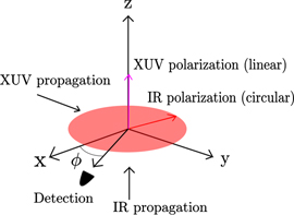
Figure 1. A schematic set-up with a linearly polarized XUV field in the z-direction and a circularly polarized IR filed in xy-plane.
Download figure:
Standard image High-resolution imageWhen such a photon is absorbed the photoelectron increases its m-value m → m + 1, and when it is emitted m → m − 1. The remaining ion will in both cases be in the state M − mi and the term determining the sideband modulation will be
If instead left-handed circularly polarized IR light is used the ϕ term in the argument will change sign. We note first that if we integrate over the azimuthal angle in (14), corresponding to full 2π detection, the signal will vanish. On the other hand a ϕ-resolved detection can replace the scan over different delays between the two light fields as a method to extract the atomic phase and attochirp [compare with (2)]. This since the atomic phase,  , will phase shift the ϕ-modulation and a comparison between atomic states or systems will reveal their relative atomic phases.
In the following we will discuss different combinations of the polarizations of the two light fields and different beam and detection geometries.
3. Results
For the numerical investigation we have used ionization from Ar(3p), and a fundamental laser frequency of ℏω = 1.55 eV, as our test case. The reduced matrix elements in (10) has been calculated using RPAE as described in references [27, 28] where it was used together with linearly polarized light.
3.1. Crossed beams
Figure 2 shows the full ϕ and θ dependence of the two-photon amplitudes with the crossed beams geometry depicted in figure 1 and discussed around equation (14). For low kinetic energies there is a node at θ = π/2, i.e. in the direction perpendicular to the XUV-polarization. For higher energies this node disappears, but reappear again for even higher energies. This is due to the Cooper minimum [35] (reached by XUV energies of ∼50 eV). Here the 3p → d one-photon channel disappears and the 3p → s one-photon channel dominates. This path is only open for electrons starting in 3pm=0 and after the subsequent interaction with a circularly polarized IR photon the final state will be exclusively of m = ±1 character, and thus with a maximum for θ = π/2.

Figure 2. The ϕ- and θ-dependence of the photoelectron amplitude for a selection of kinetic energies. The results are normalized so that the largest value in each plot is the brightest. The simulation used an XUV photon linearly polarized along the z-axis and an IR photon circularly polarized in the xy-plane, cf figure 1. The node at θ = π/2 (clearly visible in the upper left panel), i.e. for the direction perpendicular to the XUV-polarization, disappears in a broad region around the Cooper minimum (second and third upper panel). Close to the Cooper minimum the 3p → d one-photon channel disappears and the 3p → s one-photon channel dominates. This path is only open for the m = 0 state and after the subsequent interaction with a circularly polarized IR photon the final state will be exclusively of m = ±1 character, and thus with a maximum for θ = π/2.
Download figure:
Standard image High-resolution imageThe crossed-beam geometry is relevant for atoms at a fixed location in space. However, realistic RABBIT experiments always involve ensembles of atoms with a distribution extending in space over many wavelengths of the fields. This implies that atoms in the ensemble will experience a space-dependent relative delay between the fields, and that the integrated contribution of all atoms will wash out the RABBIT signal in the crossed-beam geometry.
3.2. Colinearly propagating beams
A more realistic set-up, closely resembling the traditional RABBIT one, is shown in figure 3. Here the light beams propagate in parallel and the polarization vectors of the two fields lie in the same plane. In figure 3 the XUV field is linearly polarized and the IR light is circularly polarized, but all combinations can be analyzed. Equipped with the spherical tensor operator form of the dipole operator in (15) we can combine the components to describe the geometry we are interested in. Note that
and thus linearly polarized light along the x- or y-directions can be described with the first or second line in (15) while the circularly polarized field is described by rC±1 for right-handed or left-handed polarization, respectively.
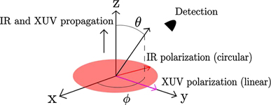
Figure 3. A schematic set-up with a linearly polarized XUV field in the y-direction and a circularly polarized IR filed in xy-plane. Both light fields propagate here in the same direction.
Download figure:
Standard image High-resolution imageFigure 4 shows the atomic delay as a function of ϕ, but for a fixed θ = π/2, for different combinations of right- and left-handed circular polarization in the xy-plane and/or linear polarization along the y-axis (cf figure 3). Note that it is now the xz-plane that is perpendicular to the linear polarization and when θ = π/2 the angle relative the polarization axis is π/2 − ϕ. The middle panel on the second line shows the classical case with both fields linearly polarized and the result for the traditional detection along the polarization axis is thus found for ϕ = π/2.

Figure 4. The atomic delay as a function of ϕ, and for θ = π/2, for ionization from Ar(3p) with different combinations of right- and left-handed circular polarization in the xy-plane (denoted by + and − respectively) and linear polarization along the y-axis, cf figure 3. The horizontal labels refer to the IR light, while the vertical labels refer to the XUV light. The different lines (solid, dotted-dashed and dashed) show three different photoelectron energies, corresponding to sideband 30, 36 and 42 (for a laser frequency of ℏω = 1.55 eV). The middle panel shows the usual setup with both fields being linearly polarized. The panels in the first and third column show the full zigzag curve from the ϕ-modulation (right y-axis) were the three lines are hard to distinguish, as well as the remaining signal when the ϕ-modulation has been removed (left y-axis). The corner panels show in this latter case a constant atomic delay for each sideband, while the left and right panels on the middle line show a remaining cos 2ϕ-modulation as expected (see text). The plots show only the region of the xy-plane where 0 < ϕ < π since since the signal repeats itself with period π. Note that the angle relative the polarization axis is here π/2 − ϕ.
Download figure:
Standard image High-resolution imageThe four corner panels in figure 4 show the atomic delay as calculated with two circularly polarized beams. The term determining the sideband modulation for the case with both light fields being right-handed will, following the discussion in section 2.2, be
where the absorption path increases the original m-value by two, while the emission path leaves it unchanged. The net effect is, as in (14) a 2ϕ-modulation. The zigzag graphs seen in figure 4 is thus the delay including the ϕ modulation

The same dependence is found for a left handed XUV photon and a right-handed IR-photon (upper right corner panel) while two left-handed fields (upper left corner panel), as well as a right-handed XUV-photon combined with a left-handed IR-photon, makes the ϕ-term change sign (bottom left corner panel). It is the polarization of the IR-field that determines the sign since it is the IR-photon that induces the ϕ-dependent phase difference in the emission path relative the absorption one. The atomic delay is in principle extractable from a ϕ-measurement just as discussed in connection with (14). Removing the 2ϕ-dependence in the corner panels reveals the underlying atomic delay and attochirp of the harmonics. In this work we assume that the attochirp is zero. The remaining atomic delay is shown as straight lines for the three calculated sidebands in the corner panels of figure 4. A similar situation has been discussed in reference [24], but for interference between a one-photon path and a two-photon path.
For the combinations of linearly polarized XUV-photons and circularly polarized IR-light shown in figure 4 the interaction with the XUV-field polarized in the y-direction can be described by the y-operator in (15) and the two-photon matrix elements, cf (5), will for + polarization of the IR-field, be proportional to

This yields several terms with different ϕ-dependence. We expect terms with no ϕ-dependence, as well as a 2ϕ-dependence and a 4ϕ-dependence:
The resulting zigzag graphs are slightly more complicated, but it is clear from figure 4 (left and right panel on the middle row) that the 2ϕ modulation dominates. When the dominating 2ϕ modulation is removed the underlying variations is revealed, as shown in the same panels.
To analyze the situation with a linearly polarized field and a circularly polarized field in the same plane it is convenient to describe the IR polarization by a field with one component parallel with the XUV polarization and one orthogonal to it: the signal from the parallel component, which gives the same situation as in the case with just linearly polarized fields, is then much larger than that from the orthogonal one. In fact the former dominates the signal in most directions as shown in the left and middle panel of figure 5 (i.e. (a) and (b)), where the two-photon amplitude modulus square is plotted against the emission ϕ-angle (for a fixed θ = π/2). The signal from the parallel component in figure 5(a) dominates over that from the orthogonal component in figure 5(b) with several orders of magnitude. For photoelectrons emitted close to the x-axis (ϕ = 0), i.e. more or less orthogonal to the XUV-polarization, the orthogonal component is dominating however, as can be seen in figure 5(c).

Figure 5. The contributions to the modulus square of the amplitude of the outgoing photoelectron, given in arbitrary units, as a function of emission angle ϕ, for the set-up in figure 3, i.e. with a linearly polarized XUV photon along the y-axis and a right-handed circularly polarized IR photon. Three different photoelectron energies are shown and θ is set to π/2. Emission parallel to the XUV polarization corresponds to ϕ = π/2 and emission perpendicular to it corresponds to ϕ = 0. (a) The contribution from the component of the IR-field that is pointing along the XUV polarization axis. (b) The contribution from the component of the IR-field that is perpendicular to the XUV polarization axis. (c) A close-up view in the vicinity of the orthogonal direction (for a photoelectron energy of 30.7 eV) where the contributions from the orthogonal IR-component is dominating.
Download figure:
Standard image High-resolution image4. Discussion
To understand the dependence on the emission angles it is illustrative to use a simple model. With a plane wave description of the photoelectron with wave vector k is
It is straight forward to analyze the angle dependence in velocity gauge since

The two-photon matrix elements [cf (5)] are in this approximation given by

where
ɛ
are complex polarization vectors of the fields. If the XUV light is polarized linearly along the y-axis,
ɛ
XUV
= (0, 1, 0), and the polarization of the IR field is right-handed in the xy-plane,  , this gives
We note that within this approximation the signal is exactly zero for ϕ = 0 (perpendicular to the XUV beam). This explains the weak signal in this direction in the numerical calculations where the non-zero, although weak effect, is caused by the presence of the Coulomb interaction. We note further that with θ = π/2, where sin θ = 1
and the combination of terms with a 4ϕ-dependence, a 2ϕ-dependence, and no ϕ-dependence, as discussed in connection with figure 4, is found.
It is also interesting to consider the variation around the XUV polarization axis i.e. around the y-axis. The cone shown in figure 6 is defined by a constant projection on the y-axis i.e. sin θ sin ϕ = c, where c is the constant. From (23) we can then conclude that

which thus is the expected θ-variation of the delay. Figure 7 shows the result (from a full numerical calculation) for three different choices of c where the signal, ∼sin2 θc2, is largest for the largest c while the delay, which has the θ-dependence predicted by (1), has its strongest angular variation when c is small. It is worth noting that if the coordinate system is rotated so that x → y, y → z and z → x, then the more familiar situation with the XUV polarization along the z-axis reappears. The IR-field will then be rotating in the yz-plane. In this case the cone is defined by the projection on the z-axis, i.e. by θ alone and it is ϕ alone that is varying when we travel around the cone.

Figure 6. The detection geometry used in figure 7. The angle with respect to the polarization vector of the linearly polarized light (along the y-axis) is kept fixed and c is the projection on the y-axis. The thick part of the circle corresponds to the x-axis in figure 7. This means that arcsin c ⩽ θ ⩽ π − arcsin c.
Download figure:
Standard image High-resolution image
Figure 7. The variation in delay (solid line left y-axis) and signal strength (dashed line right y-axis) when the electrons are detected in a direction defined by a constant angle with respect to the polarization vector of the linearly polarized light (here chosen to be along the y-axis), see figure 6. The IR-light is rotating in the xy-plane. A constant projection of the electron momentum on the y-axis is defined by sin ϕ sin θ = c, where c is constant. Three different projections are shown, all for sideband 36 corresponding to photoelectrons with an energy of 40 eV. While the signal strength increases with larger c, the angle dependence is more pronounced for smaller c. The cone intersects the xy-plane at θ = π/2 where sin ϕ = c i.e. at ϕ = π/6, π/4, π/3 for the first second and third panel respectively. The θ-axis covers arcsin c ⩽ θ ⩽ π − arcsin c, cf figure 6, and is thus different in the three cases
Download figure:
Standard image High-resolution image
The plane-wave model can also be used to analyze the combination of a linearly polarized IR field along the y-axis and a circularly polarized XUV field in the xy-plane shown in the top and bottom panels in the middle column of figure 4: here
Since the ϕ dependent argument now is the same for the absorption and emission matrix elements the formula predicts no ϕ-dependent delay and only the underlying atomic delay will be measured if the delay between the two fields are scanned. The signal strength will however vary with both ϕ and θ. The top and bottom panels in the middle coulumn of figure 4 show this situation. The rather flat delay found for ϕ close to π/2 is close to the atomic delay extracted from the other panels. At ϕ = 0 or ϕ = π (1) predicts a zero signal. The numerical calculations predicts a vanishing signal strength at these angles (not shown), but also a ϕ-variation in their neighborhood as shown in figure 4.
5. Conclusions
We have shown that with the help of angular momentum theory it is straight forward to analyze any combination of field polarizations in a RABBIT type measurement. A few possible set-ups have been analyzed here, but additional interesting combinations might still be found. With circularly polarized XUV harmonics becoming more available the possibility to use circular IR and XUV sources can be a way to facilitate the extraction of atomic delays.
Acknowledgments
The authors acknowledge support from the Knut and Alice Wallenberg Foundation, project, KAW 2017.0104, and the Swedish Research Council, Grant No. 2016-03789 and 2018-03845.