Abstract
The three-dimensional structure of Roebel cables consisting of coated conductors influences their ac loss characteristics. Measurements of the ac loss and numerical electromagnetic field analyses were carried out using a six-strand Roebel cable as well as several reference conductors: a single straight coated conductor, a 3 × 1 stack, where three straight coated conductors were stacked, and a 3 × 2 stack, where two 3 × 1 stacks were placed side by side. The measured and calculated ac losses of the Roebel cable and those of the reference conductors were compared with one another. The ac loss characteristics were discussed on the basis of the electromagnetic phenomena inside the superconductors obtained from numerical electromagnetic field analyses. The influence of the three-dimensional structure of the Roebel cable on its ac loss characteristics was verified on the basis of the experimental and numerical results.
Export citation and abstract BibTeX RIS

Content from this work may be used under the terms of the Creative Commons Attribution 3.0 licence. Any further distribution of this work must maintain attribution to the author(s) and the title of the work, journal citation and DOI.
1. Introduction
Large current-carrying capacity is required for many large-scale applications of superconductors, but the critical current (Ic) of a single high-Tc superconductor tape, such as a coated conductor, is no more than a couple of hundred amperes at 77 K and self-field. If we simply stack coated conductors to form a large-current bundle conductor, serious current imbalance among the coated conductors could affect the performance of the entire conductor unless the coated conductors are transposed somewhere in the winding to equalize the impedance among the coated-conductor strands. The Roebel cable, in which zigzag-shaped coated-conductor strands are transposed and assembled [1–5] (see figure 1), attracts broad interest as a large-current conductor. The transposition in the cable equalizes the impedance among the strands and suppresses the current imbalance among them.
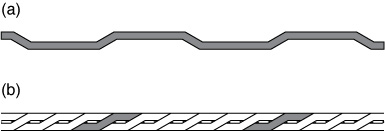
Figure 1. Schematic views of the Roebel cable: (a) strand and (b) assembled strands.
Download figure:
Standard image High-resolution imageOne of the concerns for the application of high-Tc superconductors is their ac loss because many electrical machines operate with ac. Considering that the ac loss characteristics of a superconductor are dominated by the mode of magnetic flux penetration into it, the complicated three-dimensional structure of Roebel cables could influence their ac loss characteristics. The ac loss characteristics of Roebel cables consisting of coated conductors have been studied by several groups [6–18], but the influence of their three-dimensional structure on their ac loss characteristics has not yet been well clarified.
The objective of this study is to clarify the influence of the three-dimensional structure of Roebel cables consisting of coated conductors on their ac loss characteristics. To achieve this objective, we combined experimental and numerical approaches. The experiments provided us with real values for the ac losses, which are macroscopic quantities, and the numerical electromagnetic field analyses provided us with detailed information on the electromagnetic phenomena inside the superconductors, which are related closely to the ac loss generation mechanism. The ac loss measurements were carried out using a Roebel cable consisting of six coated-conductor strands and several reference conductors. The numerical electromagnetic field analyses were also carried out using the Roebel cable and the reference conductors to study the details of the electromagnetic phenomena within them and to calculate their ac losses. For the analyses of the Roebel cable, we used our theoretical model in which the three-dimensional structure of the Roebel cable was considered [15].
This paper is organized as follows. In section 2, the details of the Roebel cables, as well as those of the reference conductors, are presented. In sections 3 and 4, the experimental methods and the model for the numerical electromagnetic field analyses are described, respectively. In section 5, the measured and analysed critical currents are shown. These critical currents are used to normalize the currents, magnetic fields and ac losses for comparison between the Roebel cable and the reference conductors with various dimensions and critical currents. In section 6, the measured and calculated ac losses of the Roebel cable and those of the reference conductors are compared with one another. The calculated electromagnetic phenomena are presented to discuss the ac loss characteristics of the Roebel cable and the reference conductors. Finally, our conclusions are presented in section 7.
2. Roebel cable and reference conductors
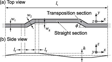
The Roebel cable consisted of six 2 mm wide strands, which were punched from 12 mm wide coated conductors fabricated by SuperPower Inc. with a 50 μm Hastelloy substrate and a 20 μm copper stabilization layer on both sides [19]. The strands were insulated on both sides by a 22 μm thick epoxy acrylate polymer. The specifications of the Roebel cable are listed in table 1 and the detailed geometry of a strand of the Roebel cable is shown in figure 2. Some parameters, which were not provided in the real sample of Roebel cable, were estimated from the other provided parameters or were assumed for the numerical electromagnetic field analyses. For example, the vertical undulation height h of a strand, which was not given explicitly in the real Roebel cable, was set at 0.5 mm so that the separation between strands did not become less than zero everywhere in the model of the Roebel cable. The top view of the Roebel cable and the cross-sectional view of its straight section are shown in figure 3(a).

Figure 2. Detailed geometry of a strand of the Roebel cable [15]. The parameters that determine the geometry are listed in table 1.
Download figure:
Standard image High-resolution image
Figure 3. Top and cross-sectional views of the Roebel cable and reference conductors: (a) Roebel cable, (b) single straight coated conductor, (c) 3 × 1 stack and (d) 3 × 2 stack.
Download figure:
Standard image High-resolution imageTable 1. Specifications of the Roebel cable.
| Strand width of the straight section (w1) | 2 mm |
| Strand width of the transposition section (w2) | 2 mm |
| Thickness of the Hastelloy substrate |
50 μm |
| Thickness of the superconductor layer (ts) |
1 μm |
| Thickness of the copper stabilization layer (on each side) |
20 μm |
| Thickness of the insulation layer of the epoxy acrylate polymer (on each side) |
22 μm |
| Minimum separation between the superconductor layers in a stack of strands |
0.135 mm |
| Gap between stacks of strands in the straight section (wg) | 1 mm |
| Transposition length (cabling pitch) (lt) | 90 mm |
| Length of the flat straight section (lf) |
2 mm |
| Roebel angle (θ) | 30° |
| Vertical undulation height (h) |
0.5 mm |
| Number of strands | 6 |
aGiven in [19]. bMean measured value. cEstimated from the thicknesses of the Hastelloy substrate, copper stabilization layers and insulation layers. dAssumed for the model for numerical electromagnetic field analyses. eAssumed so that the separation between the strands does not become less than zero everywhere in the model of the Roebel cable for numerical electromagnetic field analyses.
Three reference conductors were prepared using 4 mm wide coated conductors fabricated by SuperPower Inc. with a 50 μm Hastelloy substrate and a 20 μm copper stabilization layer on both sides [19]. These reference conductors were: a single straight coated conductor; a 3 × 1 stack, where three straight coated conductors were stacked, and a 3 × 2 stack, where two 3 × 1 stacks were placed side by side. Their top views as well as their cross-sectional views are shown in figures 3(b)–(d), respectively, and their specifications are listed in table 2. The cross section of the 3 × 2 stack was similar to that of the straight (not-transposed) section of the six-strand Roebel cable. Although the cross section of the 3 × 2 stack did not vary along its axis, the cross section of the Roebel cable varied along its axis. Polyimide sheets were placed between the coated conductors in the 3 × 1 and 3 × 2 stacks for electrical insulation. The separation between the superconductor layers of the coated conductor and that between the two 3 × 1 stacks in the 3 × 2 stack were adjusted to 0.266 mm and 2 mm, respectively. Thus, the cross section of the 3 × 2 stack consisting of 4 mm wide coated conductors was nearly proportional to that of the straight section of the Roebel cable consisting of 2 mm wide strands.
Table 2. Specifications of the reference single coated conductor, 3 × 1 stack and 3 × 2 stack.
| Width of the coated conductor | 4 mm |
| Thickness of the Hastelloy substrate |
50 μm |
| Thickness of the superconductor layer (ts) |
1 μm |
| Thickness of the copper stabilization layer (on each side) |
20 μm |
| Separation between superconductor layers in the 3 × 1 and 3 × 2 stacks |
0.266 mm |
| Gap between 3 × 1 stacks in the 3 × 2 stack | 2 mm |
aGiven in [19]. bEstimated from the thicknesses of the Hastelloy substrate, copper stabilization layers and the polyimide sheets.
3. Experimental methods
The setup for the ac loss measurement is shown schematically in figure 4 [20]. The sample conductor is placed in a dipole magnet, which applies an ac transverse magnetic field to the sample conductor. An ac transport current can be supplied to the sample conductor in the dipole magnet. In all experiments reported in this paper, the applied magnetic field was normal to the wide face of the conductor. The frequency of the current and the magnetic field was fixed at 65.44 Hz.
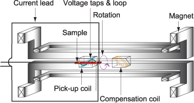
Figure 4. Setup for the ac loss measurement. © 2014 IEEE. Reprinted with permission, from [21].
Download figure:
Standard image High-resolution imageThe magnetization loss can be measured using the linked pick-up coil (LPC) installed around the sample conductor [20]. Here, its height, the length of its one turn along the sample conductor and its number of turns are denoted by hpc, L and N, respectively. In a sample consisting of n strands (n coated conductors), the magnetization loss per unit length of strand (coated conductor) per cycle, which is denoted by Qm, is given as follows:

where C is the calibration factor of the LPC determined by its cross-sectional shape, Hrms is the applied transverse magnetic field, Vm, rms is the loss component of the LPC output voltage measured with a lock-in amplifier and f is the frequency of the applied transverse magnetic field.
The transport loss can be measured by the four-probe method using spiral voltage loops [22]. In a sample consisting of n strands (n coated conductors), a pair of voltage taps associated with the spiral voltage loop is attached to each strand (coated conductor) [6, 16]. Then, the transport loss per unit length of strand (coated conductor) per cycle, which is denoted by Qt, is given as follows:
where It, entire, rms is the transport current of the entire sample conductor, d is the separation between two voltage taps, f is the frequency of the transport current and Vt, rms, k is the loss component of the voltage across two voltage taps attached to the kth strand (coated conductor) measured with the lock-in amplifier. d was 90 mm in all experiments. All strands were connected in parallel in the Roebel cable, whereas all coated conductors were connected in series to ensure uniform current distribution in the 3 × 1 and 3 × 2 stacks.
The ac loss in the sample conductor that carries an ac current in the ac transverse magnetic field, which is denoted by Qtotal, is given by the sum of Qm and Qt.
4. Theoretical model for electromagnetic field analyses
The governing equations for the numerical electromagnetic field analyses consist of Faraday's law and Biot–Savart's law:

These equations can be formulated using the current vector potential  instead of the current density
  :
:

In the magneto-quasi-static approximation of Maxwell's equations, Ampère's law holds and, thus, there exists a potential for satisfying equation (5). The extended Ohm's law, where the nonlinear equivalent conductivity σ of a superconductor replaces the constant conductivity, is used as the constitutive relation [23, 24]:
Combining equation (3) with equations (4)–(6) yields
where and  are the current vector potentials at the field point (the point where the field (potential) is calculated) and the source point (the point where a current flows to generate the magnetic field at the field point), respectively.
  is the vector from the source point to the field point and
  is the external magnetic field applied from outside the domain of integration V' of the Biot–Savart term. Because the superconductor layer of the coated conductor is very thin, we apply the thin-strip approximation [25]. The magnetic field component tangential to the superconductor layer is neglected and only the normal magnetic field component is taken into account, which dominates the ac loss in the coated conductor. In this case, is normal to the superconductor layer. and can be written as
  and
and  , where
  and
and  are the normal vectors of the superconductor layer at the field and source points, respectively. Then, we obtain
where ts is the thickness of the superconductor layer, S' is the entire area (wide face) of the superconductor layers on which the source current flows in all the strands of the Roebel cable or in all the coated conductors in the reference conductor and is the external magnetic field applied from outside the Roebel cable or the reference conductor. The three-dimensional geometry of each coated conductor is retained in the modelling in spite of the thin-strip approximation. The superconductor layer for each coated conductor is modelled as a thin curved surface that follows the three-dimensional shape of the coated conductor [15, 26, 27]. Equation (8) consists of and ; and vary on curved superconductor layers. The relative position of a field point to a source point in the three-dimensional space is represented by the vector . In this way, the three-dimensional geometry of the Roebel cable can be modelled by using scalar potentials T and T' on a mathematically two-dimensional analysis region. Galerkin's method using three-node triangular elements and a linear interpolation formula for each element is applied to discretize equation (8) spatially. The details of the modelling are described in [15], though a simplified interpolation is used for the numerical integration in the spatial discretization in the model of this paper.
The current I transported through the superconductor layer whose cross-sectional area is S is equal to the contour integral of along its periphery C:

Considering that is normal to the superconductor layer, the line integrals along both faces of the superconductor layer are eliminated; then

where T1 and T2 are the current vector potentials at the edges of the superconductor layer. Equation (10) means that the transported current I can be given by the boundary condition of T at the edges of the superconductor layer (T1 and T2) [15, 25]. In the analyses, the boundary conditions are given to provide an identical current to all strands of the Roebel cable or to all coated conductors in a stack.
The superconducting property is given by the power law E–J characteristic [23, 24]:
where Jc is the critical current density and E0 is 10−4 V m−1. The equivalent conductivity of the superconductor  is then derived as follows:

We take into account the spatial variation in critical current density caused by the spatial variation in magnetic field. The magnetic field dependence of the local critical current density is considered by Kim's model [28] as follows:

where Jc0 is the critical current density at zero magnetic field, Bn is the local magnetic flux density normal to the superconductor layer and B0 is a constant that determines the magnetic field dependence of the critical current density.
The critical current density near the edges of the coated conductors has been known to degrade often during the fabrication and/or cutting processes [29–32]. Therefore, we assumed the trapezoidal lateral Jc0 distribution with shoulders of 0.1 mm as well as the uniform lateral Jc0 distribution as shown in figure 5 in the analyses.
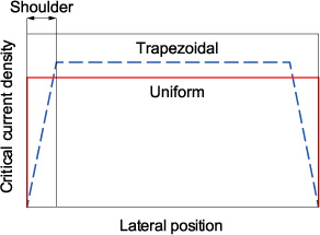
Figure 5. Uniform and trapezoidal lateral Jc0 distributions of the coated conductor. In the trapezoidal distribution, Jc0 linearly falls to zero (100% reduction) near the edges of a coated conductor.
Download figure:
Standard image High-resolution imageFinally, the ac loss power density per unit volume P can be calculated as follows:

5. Measured and analysed critical currents
5.1. Measured critical currents
In figure 6, the measured critical current of the single coated conductor at 77 K is plotted against the magnetic field, which is normal to its wide face; its critical current and n at self-field are 112.8 A and 41, respectively. The critical currents of the coated conductors in the 3 × 1 and 3 × 2 stacks were measured at self-field (before their assembly) and after their assembly. After their assembly, all coated conductors in the stack were connected in series and fed a current to ensure uniform current distribution among the coated conductors. Then, the critical current of each coated conductor was measured when the coated conductor was exposed to the magnetic fields generated by the currents in the other coated conductors. The critical current measured at self-field is denoted by Ic0 and that measured after assembly is denoted by Ic1. For the Roebel cable, Ic0 as well as n at self-field conditions of each strand was measured, but Ic1 could not be measured because the sample burned out after the ac loss measurement. The measured Ic0, Ic1 and the reduction ratio of critical current (Ic1/Ic0) in the coated conductors in the 3 × 1 and 3 × 2 stack, as well as the measured Ic0 in the strands of the Roebel cable, are listed in table 3. Using Ic1/Ic0 for the 3 × 2 stack, we estimated the Ic1 in the strands of the Roebel cable to be 34.2 A from its Ic0.

Figure 6. Critical current (Ic) of the single coated conductor versus the magnetic flux density (B) normal to its wide face: measured Ic–B data (the Ic and n at self-field are 112.8 A and 41, respectively); calculated Ic–B curves to fit the measured data assuming that n = 41, Jc0 = 3.40 × 10¹⁰ A m−2 and B0 = 43 mT in equation (13) for the uniform Jc0 distribution and assuming that n = 41, Jc0 = 3.57 × 10¹⁰ A m−2, and B0 = 42 mT in equation (13) for the trapezoidal Jc0 distribution, JcS, where Jc is the determined critical current density and S is the cross-sectional area of the superconductor layer.
Download figure:
Standard image High-resolution imageTable 3. Measured critical currents in the coated conductors in the 3 × 1 stack, 3 × 2 stack and the strands of the Roebel cable.
| Mean critical current | Reduction ratio of the critical current (Ic1/Ic0) | ||
|---|---|---|---|
| At self-field (before assembly) (Ic0) | After assembly (Ic1) | ||
| 3 × 1 stack |
110.8 A | 88.7 A | 0.801 |
| 3 × 2 stack |
111.1 A | 89.9 A | 0.809 |
| Roebel cable | 42.3 A |
34.2 A (estimated) |
0.809 (assumed) |
aCoated conductors in the 3 × 1 and 3 × 2 stacks are similar to the single coated conductor whose critical current is shown in figure 6. bMeasured n of strands of the Roebel cable are 16–33. cEstimated from Ic0 and Ic1/Ic0 for the 3 × 2 stack.
5.2. Analysed critical currents
Initially, the field-dependent critical current density in the single coated conductor was determined to reproduce the measured Ic–B data in figure 6. The critical current of a coated conductor divided by its cross-sectional area cannot provide its critical current density because of the self-field effect: the self magnetic field affects the local critical current densities. Using various values of Jc0 and B0 in equation (13), Ic can be calculated by numerical electromagnetic field analysis when the transport currents are increased slowly. The combination of Jc0 and B0 with which the calculated Ic–B curve fits well with the measured Ic–B data can be determined, while fixing n at 41 and assuming the uniform or trapezoidal Jc0 distribution. In the case of the uniform Jc0 distribution, when Jc0 and B0 were 3.40 × 10¹⁰ A m−2 and 43 mT, respectively, the calculated Ic–B curve agreed well with the measured Ic–B data as shown in figure 6. In the case of the trapezoidal Jc0 distribution, when Jc0 and B0 were 3.57 × 10¹⁰ A m−2 and 42 mT, respectively, the calculated Ic–B curve agreed well with the measured Ic–B data. The determined values of B0, which are 43 mT for the uniform Jc0 distribution and 42 mT for the trapezoidal Jc0 distribution, were used in all analyses reported in this paper. Figure 6 also shows the JcS–B curve, where Jc is calculated with the determined Jc0 and B0 using equation (13), and S is the cross-sectional area of the superconductor layer. In the case of the trapezoidal Jc0 distribution, the effective cross-sectional area considering the shoulders in the Jc0 distribution was used. Because of the self-field effect, Ic0 is apparently less than Jc0S.
Next, Jc0 was determined for the coated conductors in the 3 × 1 stack and for those in the 3 × 2 stack, assuming the uniform Jc0 distribution or the trapezoidal one. Numerical electromagnetic field analyses were carried out for the isolated coated conductor to fit the calculated Ic0 to the measured Ic0 while Jc0 was varied; n and B0 were fixed at 41 and 43 mT (42 mT), respectively. Ic1 was calculated using the determined Jc0, whereas n and B0 were the same as those at self-field.
Finally, Jc0 was determined for the strands of the Roebel cable, assuming the uniform Jc0 distribution or the trapezoidal one. Numerical electromagnetic field analyses were carried out for the isolated strand to fit the calculated Ic0 to the measured Ic0 while Jc0 was varied; n and B0 were fixed at 30 and 43 mT (42 mT), respectively. Ic1 was calculated using the determined Jc0, whereas n and B0 were the same as those at self-field.
The determined values of Jc0 and B0, the calculated values of Ic0 and Ic1, and the assumed value of n are summarized in tables 4 and 5. In the case of the trapezoidal Jc0 distribution, Jc0 in the tables denotes the Jc0 at the flat top.
Table 4. Parameters representing the superconducting properties of the single coated conductor, coated conductors in a 3 × 1 stack and coated conductors in a 3 × 2 stack for the numerical electromagnetic field analyses.
| Single coated conductor | Coated conductor in the 3 × 1 stack | Coated conductor in the 3 × 2 stack | |
|---|---|---|---|
| n | 41 | ||
| Lateral critical current density (Jc0) distribution | Uniform | ||
| Constant B0 in Kim's model |
43 mT | ||
| Critical current density at zero field (Jc0) | 3.40 × 10¹⁰ A m−2 | 3.32 × 10¹⁰ A m−2 | 3.33 × 10¹⁰ A m−2 |
| Calculated critical current at self-field (Ic0) | 113.0 A | 110.7 A | 111.0 A |
| Mean calculated critical current after assembly (Ic1) | — | 91.6 A | 91.7 A |
| Lateral critical current density (Jc0) distribution | Trapezoidal, shoulder = 0.1 mm | ||
| Constant B0 in Kim's model |
42 mT | ||
| Critical current density at zero field (Jc0) |
3.57 × 10¹⁰ A m−2 | 3.49 × 10¹⁰ A m−2 | 3.50 × 10¹⁰ A m−2 |
| Calculated critical current at self-field (Ic0) | 113.0 A | 110.9 A | 111.1 A |
| Mean calculated critical current after assembly (Ic1) | — | 91.4 A | 91.5 A |
aKim's model: Jc(Bn) = Jc0{B0/(B0 + |Bn|)}. bJc0 at the flat top.
Table 5. Parameters representing the superconducting properties of a strand of the Roebel cable for numerical electromagnetic field analyses.
| n | 30 |
|---|---|
| Lateral critical current density (Jc0) distribution | Uniform |
| Constant B0 in Kim's model |
43 mT |
| Critical current density at zero field (Jc0) | 2.44 × 10¹⁰ A m−2 |
| Calculated critical current at self-field (Ic0) | 42.3 A |
| Calculated critical current after assembly (Ic1) | 39.4 A |
| Lateral critical current density (Jc0) distribution | Trapezoidal, shoulder = 0.1 mm |
| Constant B0 in Kim's model |
42 mT |
| Critical current density at zero field (Jc0) |
2.62 × 10¹⁰ A m−2 |
| Calculated critical current at self-field (Ic0) | 42.3 A |
| Calculated critical current after assembly (Ic1) | 36.3 A |
aKim's model: Jc(Bn) = Jc0{B0/(B0 + |Bn|)}. bJc0 at the flat top.
6. Ac loss characteristics and electromagnetic phenomena
6.1. Analytical formulae for the ac losses and normalization of the ac losses
In this section, the measured and calculated ac losses per strand of the Roebel cable and per coated conductor in the reference conductors are compared with one another and with the analytical values of the ac loss for the superconductor strip. When calculating ac losses, we assumed the trapezoidal Jc0 distribution with shoulders of 0.1 mm as well as the uniform Jc0 distribution as mentioned in section 4 (figure 5). The analytical formula for the ac loss in the unit length of a superconductor strip carrying an ac current whose magnitude is It is given by Norris as follows [33]:
Meanwhile, the analytical formula for the ac loss in the unit length of a superconductor strip exposed to an ac magnetic field normal to the strip whose magnitude is Hext is given by Brandt and Indenbom as follows [34]:
and w is the width of the superconductor strip. and Qt, N−s and Qm, BI are ac losses per cycle.
Because the dimensions and the critical currents of the strands of the Roebel cable and the coated conductors in the reference conductors are different, we have to normalize the ac losses, transport currents and applied magnetic fields to compare the ac loss characteristics. Considering equations (15) and (16), It is normalized by Ic1, Qt is normalized by  , Hext is normalized by Ic1/πw and Qm is normalized by (μ0Hext)2πw2/μ0. Qtotal is also normalized by (μ0Hext)2πw2/μ0 when it is plotted against Hext/(Ic1/πw). In the case of the single coated conductor, Ic1 is replaced with Ic0. It/Ic1, Hext/(Ic1/πw), Qm/{(μ0Hext)2πw2/μ0} and Qtotal/{(μ0Hext)2πw2/μ0} are dimensionless, while the dimension of
  is J m−1 A−2. The measured ac losses of the Roebel cable are the same as those reported in [16] but are normalized for the comparison.
6.2. Roebel cable and reference conductors carrying ac current
Figure 7 shows the plot of the normalized transport losses per coated conductor (strand) against the normalized transport current: the losses were calculated with the uniform Jc0 distribution in figure 7(a) and were calculated with the trapezoidal Jc0 distribution in figure 7(b). In the Roebel cable and the 3 × 2 stack, the measured transport losses agree well with the transport losses calculated with the uniform Jc0 distribution as well as those calculated with the trapezoidal Jc0 distribution. In other words, the variations in their Jc0 distributions to this extent hardly influence their transport losses. In the single coated conductor and the 3 × 1 stack, the transport losses calculated with the trapezoidal Jc0 distribution are larger than the measured ones when It/Ic1 ≤ 0.3, whereas those calculated with the uniform Jc0 distribution agree well with the measured ones even in this small current region. The Jc0 distributions in these two samples might be rather uniform. However, the alignment of coated conductors in the 3 × 1 stack might also influence its transport loss in the small current region. The comparison among the transport losses of the Roebel cable and the reference conductors can be summarized as follows:
- (1)The transport loss of the single coated conductor is the smallest and almost agrees with Qt, N−s. This result can be understood naturally.
- (2)The transport loss of the 3 × 1 stack is slightly smaller than that of the 3 × 2 stack as well as that of the Roebel cable.
- (3)The transport loss of the Roebel cable and that of the 3 × 2 stack are almost the same [7].
To discuss the transport loss characteristics, the lateral magnetic flux density distributions at the peak phase of the transport current, which are obtained from the results of the numerical electromagnetic field analyses, are shown in figure 8 when It/Ic1 = 0.4, where the trapezoidal Jc0 distribution is assumed. The magnetic flux density is normalized by μ0Ic1/π. Figures 8(a)–(c) show the distributions in the straight section of the Roebel cable, in the 3 × 2 stack and in the 3 × 1 stack, respectively. We selected the trapezoidal Jc0 distribution, because the ac losses calculated with this distribution reproduce the measured ac losses better, when looking at the entire results in this paper. The lateral magnetic flux density distributions calculated with the uniform Jc0 distribution shown in the appendix are similar to those in figure 8.

Figure 7. Measured and calculated transport losses normalized by versus transport current normalized by Ic1: (a) the uniform Jc0 distribution was used for calculations and (b) the trapezoidal Jc0 distribution was used for calculations.
Download figure:
Standard image High-resolution image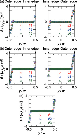
Figure 8. Lateral distribution of the magnetic flux density normalized by μ0Ic1/πw at peak phase when It/Ic1 = 0.4, where the trapezoidal Jc0 distribution is assumed: (a) Roebel cable, (b) 3 × 2 stack and (c) 3 × 1 stack. #1–#6 denote the strands (coated conductors).
Download figure:
Standard image High-resolution imageIn the 3 × 1 stack in figure 8(c), the magnetic flux penetrates equally from both edges of the coated conductors. In the 3 × 2 stack in figure 8(b), more magnetic flux penetrates from the outer edges of the coated conductors, but a considerable amount of magnetic flux penetrates from the inner edges. The gap between the two 3 × 1 stacks in the 3 × 2 stack is half the width of the coated conductor. This relatively large gap might have caused the magnetic flux penetration from the inner edges of the coated conductors, which is approximately comparable with that from the outer edges. It could be the reason why the transport loss of the 3 × 2 stack is comparable with that of the 3 × 1 stack, as pointed out by item (2) above.
Item (3) appears reasonable if we compare the structure of the straight section of the Roebel cable with that of the 3 × 2 stack. The lateral magnetic flux density distributions in the straight section of the Roebel cable (figure 8(a)) are similar to that in the 3 × 2 stack (figure 8(b)). Even in the Roebel cable where the strands are interlaced, the magnetic flux can penetrate from the inner edges of the strands as well as from their outer edges. Therefore, if we look at the straight section of the Roebel cable only, its ac loss characteristics might appear similar to that of the 3 × 2 stack.
However, if we consider the three-dimensional structure of the Roebel cable, this situation is not as straightforward as described above. In the Roebel cable, transposition sections (where the strands are transposed) exist as well as straight sections. The longitudinally modulated structure of the Roebel cable must result in longitudinal variations in the current and magnetic flux density distributions and in the ac loss generation. Figures 9(a)–(c) show the current lines on the strand, the ac loss energy density distribution on the strand and the ac loss energy distribution along the strand axis for a quarter transposition length (cabling pitch) of a strand, respectively, when It/Ic1 = 0.4, where the trapezoidal Jc0 distribution is assumed. Similar figures with the uniform Jc0 distribution are shown in the appendix. A quarter transposition length is sufficient for illustration because of the periodicity of the Roebel cable structure. Figure 10 shows a similar figure when It/Ic1 = 0.8. In figures 9(a) and 10(a), the current lines are distorted in the transposition section of the other strands. In the transposition section of the other strands in figures 9(a) and 10(a), the current concentrates near the outer side because of the shielding from the magnetic field generated by the currents in the other strands. Therefore, in figure 10(b), a concentration of ac loss generation is observed near the outer edge of the strand in the transposition section of the other strands. In the transposition section of the strand itself where the strand is located at the centre of the Roebel cable in figures 9(a) and 10(a), the magnetic flux (current) naturally penetrates equally from both edges of the strand; a less concentrated magnetic flux penetration results in smaller ac loss generation. Figures 9(c) and 10(c) more remarkably show the spatial variation in the ac loss generation; a larger ac loss is generated in the transposition section of the other strands and a smaller ac loss is generated in the transposition section of the strand itself. The larger and smaller ac loss regions compensate each other and the transport loss averaged along the transposition length is almost the same as that of the 3 × 2 stack, as shown in figure 7.
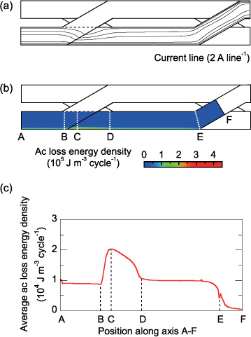
Figure 9. Current and ac loss energy distribution in a strand of the Roebel cable when It/Ic1 = 0.4, where the trapezoidal Jc0 distribution is assumed: (a) current lines on a strand at peak phase, (b) ac loss energy density distribution on a strand and (c) ac loss energy distribution along the strand axis.
Download figure:
Standard image High-resolution image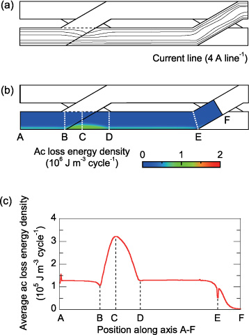
Figure 10. Current and ac loss energy distribution in a strand of the Roebel cable when It/Ic1 = 0.8, where the trapezoidal Jc0 distribution is assumed: (a) current lines on a strand at peak phase, (b) ac loss energy density distribution on a strand and (c) ac loss energy distribution along the strand axis.
Download figure:
Standard image High-resolution image6.3. Roebel cable and reference conductors exposed to an ac magnetic field
Figure 11 shows the plot of the normalized magnetization losses per coated conductor (strand) against the normalized applied magnetic field: the losses were calculated with the uniform Jc0 distribution in figure 11(a) and were calculated with the trapezoidal Jc0 distribution in figure 11(b). The measured magnetization losses agree better with the magnetization losses calculated with the trapezoidal Jc0 distribution as shown in figure 11(b), except for the single coated conductor in a very small field region (Hext/(Ic1/πw) < 0.3). Similar to section 6.2, we summarize the comparison among the magnetization losses of the Roebel cable and the reference conductors as follows:
- (1)The magnetization loss of the single coated conductor is the largest and almost agrees with Qm, BI.
- (2)The magnetization loss of the 3 × 2 stack is comparable with that of the 3 × 1 stack over the entire range of the magnetic field.
- (3)In the large field region (7 ≤ Hext/(Ic1/πw)), where the demagnetization effect is negligible, the magnetization losses of the Roebel cable, 3 × 2 stack, 3 × 1 stack and single coated conductor reasonably agree with one another.
- (4)In the middle field region (2 ≤ Hext/(Ic1/πw) < 7), the magnetization losses of the Roebel cable, 3 × 2 stack and 3 × 1 stack reasonably agree with one another; they are smaller than the magnetization loss of the single coated conductor.
- (5)In the small field region (Hext/(Ic1/πw) < 2), the magnetization loss of the Roebel cable deviates from those of the 3 × 2 and 3 × 1 stacks; it becomes larger with decreasing magnetic field.
The calculated lateral magnetic flux density distributions are shown in figures 12(a), (b) and (c) for the straight section of the Roebel cable, for the 3 × 2 stack and for the 3 × 1 stack, respectively, when Hext/(Ic1/πw) = 3.2, where the trapezoidal Jc0 distribution is assumed. In figures 13–15, the current lines on the strand, the ac loss energy density distribution on the strand and the ac loss energy distribution along the strand axis are shown for a quarter transposition length of the strand when Hext/(Ic1/πw) = 0.5, 3.2 and 7, respectively, where the trapezoidal Jc0 distribution is assumed. Similar figures with the uniform Jc0 distribution are shown in the appendix.
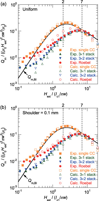
Figure 11. Measured and calculated magnetization losses normalized by (μ0Hext)2πw2/μ0 versus magnetic field normalized by Ic1/πw: (a) the uniform Jc0 distribution was used for calculations and (b) the trapezoidal Jc0 distribution was used for calculations.
Download figure:
Standard image High-resolution image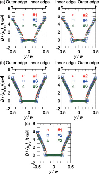
Figure 12. Lateral distribution of the magnetic flux density normalized by μ0Ic1/πw at peak phase when Hext/(Ic1/πw) = 3.2, where the trapezoidal Jc0 distribution is assumed: (a) Roebel cable, (b) 3 × 2 stack and (c) 3 × 1 stack. #1–#6 denote the strands (coated conductors).
Download figure:
Standard image High-resolution image
Figure 13. Current and ac loss energy distribution in a strand of the Roebel cable when Hext/(Ic1/πw) = 0.5, where the trapezoidal Jc0 distribution is assumed: (a) current lines on a strand at peak phase, (b) ac loss energy density distribution on a strand and (c) ac loss energy distribution along the strand axis.
Download figure:
Standard image High-resolution image
Figure 14. Current and ac loss energy distribution in a strand of the Roebel cable when Hext/(Ic1/πw) = 3.2, where the trapezoidal Jc0 distribution is assumed: (a) current lines on a strand at peak phase, (b) ac loss energy density distribution on a strand and (c) ac loss energy distribution along the strand axis.
Download figure:
Standard image High-resolution image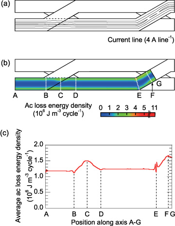
Figure 15. Current and ac loss energy distribution in a strand of the Roebel cable when Hext/(Ic1/πw) = 7, where the trapezoidal Jc0 distribution is assumed: (a) current lines on a strand at peak phase, (b) ac loss energy density distribution on a strand and (c) ac loss energy distribution along the strand axis.
Download figure:
Standard image High-resolution imageBecause the two 3 × 1 stacks in the 3 × 2 stack are insulated electrically from each other, the two stacks cannot be coupled electromagnetically. Because of the relatively large gap between them, the effects of demagnetization from the other stack is small. Figures 12(b) and (c) show that the magnetic flux density distributions in the 3 × 1 and 3 × 2 stacks are almost the same. Therefore, the magnetization loss of the 3 × 2 stack is comparable with that of the 3 × 1 stack, as pointed out in item (2) above.
Iwakuma et al reported the agreement between the magnetization loss of a single coated conductor and that of stacks of coated conductors in a high field region, as well as smaller magnetization losses in the stacks compared to that in a single coated conductor in a smaller field region [35].
The magnetization loss of the Roebel cable almost agrees with that of the 3 × 2 stack in the large and middle field regions (2 ≤ Hext/(Ic1/πw)), as shown in figure 11. This result appears reasonable if we compare the structure of the straight section of the Roebel cable with that of the 3 × 2 stack. Because the strands are insulated electrically from one another, no coupling current (which shields the applied magnetic field) can flow. Therefore, although the strands are interlaced, the magnetic flux can penetrate from the inner edges of the strands; the lateral magnetic flux density distributions in the straight section of the Roebel cable (figure 12(a)) are similar to the lateral magnetic flux density distributions in the 3 × 2 stack (figure 12(b)).
However, we must consider the three-dimensional structure of the Roebel cable with transposition sections as well as straight sections. When the applied magnetic field is large (Hext/(Ic1/πw) = 7), the current flows mostly parallel to the strand axis, as shown in figure 15(a). Meanwhile, when the applied magnetic field is smaller (Hext/(Ic1/πw) = 0.5,3.2), the current lines are remarkably distorted in the transposition section of the other strands and in the transposition section of the strand itself, as shown in figures 13(a) and 14(a). When a strand is not saturated, more current must flow in the strand to shield the applied magnetic field in the transposition section where the number of stacked strands is two, as compared to the straight section where the number of stacked strands is three. Circulating currents are observed in the transposition sections in figures 13(a) and 14(a). These additional circulating shielding currents lead to the concentrations of ac loss generation observed in figures 13(b), (c), 14(b) and (c). The longitudinal variation in the ac loss generation is more remarkable at lower applied magnetic fields (see figures 13(c), 14(c) and 15(c)). The large ac loss generation in the transposition section results in larger magnetization losses in the Roebel cable than those in the 3 × 2 stack in the small field region, as shown in figure 11.
6.4. Roebel cable and reference conductors carrying ac current and exposed to an ac magnetic field
Figure 16 shows the plot of the normalized ac losses per coated conductor (strand) against the normalized applied magnetic field when the conductor carries an ac current in an ac magnetic field: the losses were calculated with the uniform Jc0 distribution in figure 16(a) and were calculated with the trapezoidal Jc0 distribution in figure 16(b). Especially in the Roebel cable, the measured ac losses agree better with the ac losses calculated with the trapezoidal Jc0 distribution, as shown in figure 16(b). The comparison among the ac losses of the Roebel cable and the reference conductors are summarized as follows:
- (1)In the large field region (7 ≤ Hext/(Ic1/πw)), where the applied magnetic field dominates the ac losses and the demagnetization effect is negligible, the ac losses of the Roebel cable, 3 × 2 stack, 3 × 1 stack and single coated conductor almost agree with one another.
- (2)In the middle field region (0.5 ≤ Hext/(Ic1/πw) < 7), the ac losses of the Roebel cable, 3 × 2 stack and 3 × 1 stack roughly agree with one another; they are smaller than that of the single coated conductor.
- (3)In the small field region (Hext/(Ic1/πw) < 0.5), where the self magnetic field due to the transport current dominates the ac losses, the ac losses of the Roebel cable, 3 × 2 stack and 3 × 1 stack roughly agree with one another; they are larger than that of the single coated conductor.
The calculated lateral magnetic flux density distributions in the straight section of the Roebel cable, in the 3 × 2 stack and in the 3 × 1 stack are shown in figures 17(a), (b) and (c), respectively, when It/Ic1 = 0.6 and Hext/(Ic1/πw) = 2, where the trapezoidal Jc0 distribution is assumed. Figure 18 shows the current lines on the strand, the ac loss energy density distribution on the strand and the ac loss energy distribution along the strand axis for a half transposition length of the strand when It/Ic1 = 0.6 and Hext/(Ic1/πw) = 2, where the trapezoidal Jc0 distribution is assumed. Similar figures with the uniform Jc0 distribution are shown in the appendix.
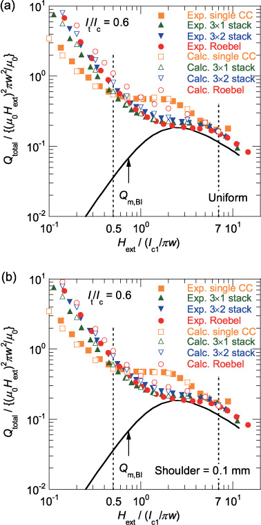
Figure 16. Measured and calculated ac losses normalized by (μ0Hext)2πw2/μ0 versus the magnetic field normalized by Ic1/πw when the conductors carry an ac current and are exposed to an ac magnetic field: (a) the uniform Jc0 distribution was used for calculations and (b) the trapezoidal Jc0 distribution was used for calculations.
Download figure:
Standard image High-resolution image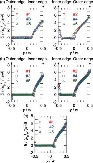
Figure 17. Lateral distribution of the magnetic flux density normalized by μ0Ic1/πw at peak phase when It/Ic1 = 0.6 and Hext/(Ic1/πw) = 2, where the trapezoidal Jc0 distribution is assumed: (a) Roebel cable, (b) 3 × 2 stack and (c) 3 × 1 stack. #1–#6 denote the strands (coated conductors).
Download figure:
Standard image High-resolution image
Figure 18. Current and ac loss energy distribution in a strand of the Roebel cable when It/Ic1 = 0.6 and Hext/(Ic1/πw) = 2, where the trapezoidal Jc0 distribution is assumed: (a) current lines on a strand at peak phase, (b) ac loss energy density distribution on a strand and (c) ac loss energy distribution along the strand axis.
Download figure:
Standard image High-resolution imageThe ac loss characteristics in the large and small field regions are analogous to the magnetization loss characteristics presented in section 6.3 and to the transport loss characteristics presented in section 6.2, respectively. The middle field region (0.5 ≤ Hext/(Ic1/πw) < 7) attracts our interest. The ac loss in the middle field region is larger than Qm, BI owing to the influence of the transport current. The lateral magnetic flux density distribution in the straight section of the Roebel cable (figure 17(a)) is similar to that of the 3 × 2 stack (figure 17(b)). Figure 18(a) shows that the current lines are distorted in the transposition sections and hence the ac loss energy density varies remarkably along the strand axis (figure 18(c)).
7. Conclusion
Experimental and numerical approaches have been combined to study the ac loss characteristics of a Roebel cable consisting of insulated coated conductors. The agreement between the measured and numerically calculated ac losses supports the validity of the numerical electromagnetic field analyses. The current lines on the strand of the Roebel cable, illustrated based on the numerical analyses, are distorted in the transposition sections; the mode of magnetic flux penetration is influenced by the three-dimensional transposed structure of the Roebel cable. The ac loss generation is locally concentrated because of the transposition of the strands. However, except for the small field region, the ac loss of the Roebel cable averaged along its transposition length is almost the same as those of the stacks of coated conductors, which simulate bundled conductors with uniform current distribution. In other words, whereas the strands in the Roebel cables are interlaced, the ac losses of the Roebel cables can be as low as those of the bundled conductors where the strand currents are equalized by the complicated transposed windings.
Acknowledgment
This work was supported in part by the Japan Science and Technology Agency under the Strategic Promotion of Innovative Research and Development Program.
Appendix.:
The distributions of magnetic flux density, current and ac loss energy density calculated with the uniform Jc0 distribution are shown in figures A.1–A.9.
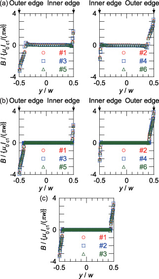
Figure A.1. Lateral distribution of the magnetic flux density normalized by μ0Ic1/πw at peak phase when It/Ic1 = 0.4, where the uniform Jc0 distribution is assumed: (a) Roebel cable, (b) 3 × 2 stack and (c) 3 × 1 stack. #1–#6 denote the strands (coated conductors). To be compared with figure 8 with the trapezoidal Jc0 distribution.
Download figure:
Standard image High-resolution image
Figure A.2. Current and ac loss energy distribution in a strand of the Roebel cable when It/Ic1 = 0.4, where the uniform Jc0 distribution is assumed: (a) current lines on a strand at peak phase, (b) ac loss energy density distribution on a strand and (c) ac loss energy distribution along the strand axis. To be compared with figure 9 with the trapezoidal Jc0 distribution.
Download figure:
Standard image High-resolution image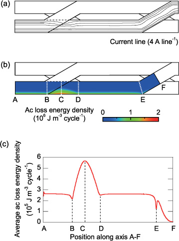
Figure A.3. Current and ac loss energy distribution in a strand of the Roebel cable when It/Ic1 = 0.8, where the uniform Jc0 distribution is assumed: (a) current lines on a strand at peak phase, (b) ac loss energy density distribution on a strand and (c) ac loss energy distribution along the strand axis. To be compared with figure 10 with the trapezoidal Jc0 distribution.
Download figure:
Standard image High-resolution image
Figure A.4. Lateral distribution of the magnetic flux density normalized by μ0Ic1/πw at peak phase when Hext/(Ic1/πw) = 3.2, where the uniform Jc0 distribution is assumed: (a) Roebel cable, (b) 3 × 2 stack and (c) 3 × 1 stack. #1–#6 denote the strands (coated conductors). To be compared with figure 12 with the trapezoidal Jc0 distribution.
Download figure:
Standard image High-resolution image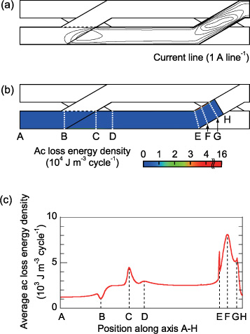
Figure A.5. Current and ac loss energy distribution in a strand of the Roebel cable when Hext/(Ic1/πw) = 0.5, where the uniform Jc0 distribution is assumed: (a) current lines on a strand at peak phase, (b) ac loss energy density distribution on a strand and (c) ac loss energy distribution along the strand axis. To be compared with figure 13 with the trapezoidal Jc0 distribution.
Download figure:
Standard image High-resolution image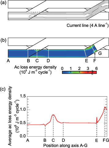
Figure A.6. Current and ac loss energy distribution in a strand of the Roebel cable when Hext/(Ic1/πw) = 3.2, where the uniform Jc0 distribution is assumed: (a) current lines on a strand at peak phase, (b) ac loss energy density distribution on a strand and (c) ac loss energy distribution along the strand axis. To be compared with figure 14 with the trapezoidal Jc0 distribution.
Download figure:
Standard image High-resolution image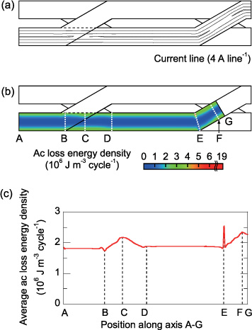
Figure A.7. Current and ac loss energy distribution in a strand of the Roebel cable when Hext/(Ic1/πw) = 7, where the uniform Jc0 distribution is assumed: (a) current lines on a strand at peak phase, (b) ac loss energy density distribution on a strand and (c) ac loss energy distribution along the strand axis. To be compared with figure 15 with the trapezoidal Jc0 distribution.
Download figure:
Standard image High-resolution image
Figure A.8. Lateral distribution of the magnetic flux density normalized by μ0Ic1/πw at peak phase when It/Ic1 = 0.6 and Hext/(Ic1/πw) = 2, where the uniform Jc0 distribution is assumed: (a) Roebel cable, (b) 3 × 2 stack and (c) 3 × 1 stack. #1–#6 denote the strands (coated conductors). To be compared with figure 17 with the trapezoidal Jc0 distribution.
Download figure:
Standard image High-resolution image
Figure A.9. Current and ac loss energy distribution in a strand of the Roebel cable when It/Ic1 = 0.6 and Hext/(Ic1/πw) = 2, where the uniform Jc0 distribution is assumed: (a) current lines on a strand at peak phase, (b) ac loss energy density distribution on a strand and (c) ac loss energy distribution along the strand axis. To be compared with figure 18 with the trapezoidal Jc0 distribution.
Download figure:
Standard image High-resolution image