
Abstract
Recent advances in manufacturing arrays of artificial pinning sites, i.e., antidots, blind holes and magnetic dots, allowed an effective control of magnetic flux in superconductors. An array of magnetic bars deposited on top of a superconducting film was shown to display different pinning regimes depending on the direction of the in-plane magnetization of the bars. Changing the sign of their magnetization results in changes in the induced magnetic pinning potentials. By numerically solving the time-dependent Ginzburg–Landau equations in a superconducting film with periodic arrays of zigzag-arranged magnetic bars, we revealed various flux dynamics regimes. In particular, we demonstrate flux pinning and flux flow, depending on the direction of the magnetization of the magnetic bars. Remarkably, the revealed different flux-motion regimes are associated with different mechanisms of vortex–antivortex dynamics. For example, we found that for an 'antiparallel' configuration of magnetic bars this dynamics involves a repeating vortex–antivortex generation and annihilation. We show that the depinning transition and the onset of flux flow can be manipulated by the magnetization of the bars and the geometry of the array. This provides an effective control of the depinning critical current that can be useful for possible fluxonics applications.
Export citation and abstract BibTeX RIS
1. Introduction
Nanoscience relies upon the modification of the properties of the same material through its nanostructuring and the optimization of the confinement potential and topology [1]. It has been shown that properties of heterostructures are significantly distinguished from those of an intrinsic superconductor (SC) [2]. Thus embedding ferromagnetic nanostructures allows one to improve the properties of a SC: the critical current (see, e.g., [3]), the critical temperature [4] and the pinning potential [5]. As a result, the range of applications of heterostructured SC is much wider than that of pure SC. The magnetic confinement permits one to control the physical properties of the confined condensates and magnetic flux. Magnetic nanostructures are especially interesting because their magnetic moments can be easily controlled, giving rise to a high degree of tunability of their flux pinning properties. This has been demonstrated in recent experiments in which arrays of nanomagnets were shown to trap vortices quite efficiently, either by local reduction of the critical temperature via the proximity effect [6, 7] or by their magnetic flux when the dots are polarized [8–10].
Controlling the vortex motion and creating a guided vortex motion [11, 12] via nanoengineering of arrays of pinning sites [13] or channels in the superconductor, makes it possible to develop new devices such as micronet superconducting transistors, switches, pumps [14], etc [15]. This paves the way for designing new generations of devices based on the controlled behavior of fluxons. The charge and the spin of electrons form the core of electronics and spintronics, respectively. In the same way, mastering fluxon behavior in nanostructured superconductors creates exciting new possibilities to develop the basics of fluxonics. By optimizing the condensate and the flux confinement, the superconducting critical parameters can be enhanced through nanostructuring.
There are a variety of nanoscale configurations used to confine flux and the condensate in nanostructured superconductors, moving from single nanocells (loop, disc, triangle, square, etc) via their clusters to their arrays (antidot lattices, etc) [16–19]. In addition to that, nanoscale magnetic templates, where highly inhomogeneous local magnetic fields were generated by ferromagnetic nanodots and magnetic domains, are considered in superconductor–ferromagnet hybrid nanosystems.
Examples of magnetic heterostructures include: thin superconducting films with thin magnetic disks on top [20], ferromagnetic square microrings [21], parallel [22] and orthogonal [23] periodic patterns of Co bars, etc (see review paper [24]). In all these systems the intense stray field generated by a magnet deposited on top of the system depletes the superconducting order parameter. This universal behavior is observed regardless of the superconductor type. In those systems the distribution of the current density in the superconductor is rather inhomogeneous, and vortex trajectories which are determined by the current density distribution, as well as by the interaction with the complex potential-energy landscape created by the defects and by the interaction with other vortices, may have very complicated shape.
In this work, we investigate the vortex–antivortex dynamics in a SC film with a rectangular array of ferromagnetic bars in a zigzag configuration (see figure 1) deposited on top. This magnetic bar configuration has been experimentally investigated in [23]. The stray field of the array of magnetic bars governs the dynamic regime of the (anti)vortex motion in an infinite SC film. It is possible to change the magnetization of the zigzag bar pattern by applying an in-plane magnetic field. Depending on the initial magnetic-field orientation, one can obtain two different magnetic-field profiles in the film. This profile will affect (anti)vortex motion in the SC film. We demonstrate that changing the set-up of the magnetic profile, we can tune the vortex system between the flux-flow (FF) and pinned regime. The simplicity of changing the magnetic profile makes this system very attractive for further experiments. As a theoretical approach, we rely upon the time-dependent Ginzburg–Landau (TDGL) equations which allow us to study self-consistently both the nucleation of the vortex–antivortex (v–av) pairs (see, e.g., [25]) and their dynamics. This provides an obvious advantage of the used method (as compared, e.g., to molecular dynamics simulations of vortices) for arrays of magnetic dots (bars) where the vortex–antivortex dynamics is accompanied by the nucleation and annihilation of v–av pairs. For example, we revealed that the mechanism of flux motion in the case of an 'antiparallel' configuration of magnetic bars is associated with a repeating generation and annihilation of vortex–antivortex pairs under the tips of adjacent bars.

Figure 1. The model system. The magnetization of the bars changes under the external magnetic field Hex and modulates differently in the central area (green (gray) dashed box). The orientation of the initial magnetic field generates ((a), (b)) antiparallel (AP) and ((c), (d)) parallel (P) configurations. Circled dots and crosses show the location of out-of-plane dipoles whose magnetic field is approximately the same as the field of the bar. The current leads are at the bottom and the top of the SC film. Itr shows the direction of the transport current flow. a denotes the distance between the neighbor bar tips (i.e., the off-plane dipoles). The meaning of the x-,y-, and z-axes is clear from the plot.
Download figure:
Standard imageThis paper is organized as follows. In section 2, we describe the model system. In section 3, we demonstrate the essential role of the magnetization of the out-of-plane dipole and its position above the surface of a SC for the vortex motion. In section 4, IV-curves of the system and various mechanisms of flux motion are analyzed. The results obtained in the present work are divided into two parts: one for a system modeled by out-of-plane dipoles and the second one by in-plane dipoles. The results with in-plane simulations are presented in section 5. Our main results and insights are summarized in section 6.
2. Model
Our system consists of a superconducting film with an array of magnetic bars deposited on top of the superconductor. Depending on the geometry of the bars (e.g., whether they are narrow or wide) and the array, the bars are modeled either by (i) out-of-plane magnetic dipoles [26], or (ii) in-plane dipoles (the typical dimensions are 3 × 32ξ). The superconducting film is assumed to be of finite length (in the direction of the leads) and of infinite width, which provides an adequate description of vortex creep in a real system. To model the infinite (in one direction) film, we use periodic boundary conditions applied to the phase and amplitude of the order SC parameter. The geometry of the system is as follows: the magnetic bars are deposited on top of a thin insulating layer (with separation z along the z-direction) of the rectangular SC film as 'ribbons' are formed under an angle of 45° with respect to the film face. Therefore, the bars in the adjacent rows form an angle of 90° with respect to each other, i.e., a 'zigzag' configuration (see figure 1). For instance, in the case of a 'narrow' magnetic bar, we model a Co bar with typical dimensions 2900 nm × 76 nm × 153 nm, separated from the superconducting film by a Ge insulator layer of thickness z = 139 nm, which provides the magnetic momentum: μ ≈ 56μ0 = 2.24 × 10⁻¹⁹ A m2, where μ0 = Φ0ξ/2π = 4 × 10⁻²¹ A m2. This system is attractive due to the simplicity of changing the direction of magnetization by applying an in-plane magnetic field.
In our simulations, we use a film with length 30ξ and width 80ξ, where ξ is the superconducting coherence length at zero temperature T. In order to (re)magnetize the bars, an in-plane uniform magnetic field is applied either along the x- or the y-direction. As a result, the bars are magnetized either in an 'antiparallel' (AP) (figures 1(a) and (b)) or in a 'parallel' (P) (figures 1(c) and (d)) configuration. It is assumed that the bars are magnetized using the field-cooled regime (FC), and after some relaxation time the generated vortices are trapped under the tips of the bars. This results in the two types of magnetic-field profile (along the lines connecting the apices of the bars) shown in figures 2(a) and (b), corresponding to the AP and P magnetization configurations (figure 1). The two generated magnetic-field profiles are quantitatively and qualitatively different: the one corresponding to the AP magnetization configuration consists of periodic sharp peaks of opposite polarity (figure 2(a)) while the one resulting from the P magnetization configuration is a twice as dense set of sharp peaks of the same polarity (figure 2(b)). Clearly, the transition from one magnetic-field configuration to the other significantly changes the condition for (anti-)vortex motion along the magnetic-field modulated 'paths' (or 'channels'). Note that the height and width of the peaks are determined by the magnetization of the bars (or the dipoles in the out-of-plane dipole model) and the separation z between the dipole and the SC film (i.e., the thickness of the insulating layer).
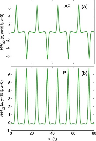
Figure 2. The magnetic-field profile Hz (x,y = 15,z = 0) induced by the dipoles. The positions of the sharp peaks represent the location of the magnetic dipole. Magnetic momentum μz = 1μ0 is strong enough to induce one v–av pair only with vorticity L = 1 for each Hc2 period. The magnetic profile is created by: (a) antiparallel dipoles and (b) parallel dipoles.
Download figure:
Standard imageAs we showed by direct calculation of the magnetic-field profile created by an in-plane magnetized bar, the real profile of the z-component of the magnetic field (which mainly affects the superconducting properties of the film) of a narrow bar could be modeled by a proper choice of the magnetization of two out-of-plane dipoles (see inset of figure 2 in [26]), the inter-dipole distance and the distance between them and the superconducting sample.
After the initial configuration of the system (i.e., the magnetic-field profile and the distribution of (anti)vortices) has been prepared, the current is turned on, and we investigate the v–av dynamics. To study the dynamics of the vortex–antivortex (v–av) pairs, we employ the time-dependent Ginzburg–Landau equation [25, 27]:

The equation is to be solved self-consistently with the Poisson equation for the electrostatic potential,

In equations (1) and (2), all the physical quantities are expressed in dimensionless units: temperature T in units of the critical temperature Tc, the vector potential A in units of Φ0/(2πξ(T)) (where Φ0 is the quantum of magnetic flux), the order parameter in units of Δ0 = 4kBTcu1/2/π(1−T/Tc)1/2, and the coordinates are in units of the coherence length ξ(T) = (8kBTc/πħD)−1/2/(1−T/Tc)1/2. Using these units, the magnetic field is scaled by Hc2 = Φ0/2πξ(T)2 and the current density by j0 = σnħ/2eτGL(T)ξ(T). Time is scaled in units of the Ginzburg–Landau relaxation time τGL(T) = πħ/8kBTcu/(1 − T/Tc), the electrostatic potential φ in units of φ0 = V0 = ħ/2eτGL(T), where σn is the normal-state conductivity, and D is the diffusion constant. Parameter u governs the time change of |ψ| and the length of penetration of the electric field into a superconductor [28]. Since we are interested mainly in the dynamics of vortex–antivortex motion but not in the time evolution of the v–av nucleation and annihilation, for our problem the actual value of u does not play an essential role, and we choose the value u = 5.79 (note that this value depends on the specific superconductor).
The vector potential in equations (1) and (2) is the sum of the vector potentials induced by magnetic dipoles which are placed at a distance z0 = 2.8ξ from the top surface of the superconducting film. We assume that the thickness of the superconducting film ds is smaller than the effective (normal) magnetic-field penetration depth, Λ = λ(T)2/ds, where ds is the thickness of the sample. Due to the fact that our system is infinite in the x-direction, there is no screening current along the y-direction. However, in a real system the influence of the screening currents on A may be omitted if the film width is smaller than Λ [29].
In the x-direction we use the usual periodic boundary conditions for the magnitude and phase of the order parameter: ψ|0 = ψ|N,φ|0 = φ|N, and in the y-direction we employ the 'normal metal–superconductor' boundary conditions: ψ = 0, ∂φ/∂n =− jn. The current is applied along the y-axis as shown in figure 1. We define the critical 'depinning' current jc as the current resulting in non-zero vortex velocity in the dynamic regime. The typical value of the critical voltage (which corresponds to the threshold voltage to determine the critical depinning current) corresponds to 2.0 × 10⁻⁴φ0.
The numerical solution of the TDGL equations is obtained using the finite-difference method, the Fourier analysis and the cyclic reduction method (FACR) [30–32].
3. Magnetic-field profile of an array of out-of-plane dipoles
Let us first consider the central region of the sample limited by dashed lines in figures 1(a) and (b). This region contains one 'channel' with a modulated magnetic-field profile. We assume that magnetic bars are long, narrow (∼1D) and well separated. These magnetic bars induce local and non-overlapping regions of depleted order parameter.
A contour plot of the order parameter for a single chain of eight dipoles in the equilibrium state will be discussed in section 4.2, see figure 6(a). In the absence of applied current, the equilibrium state is a set of pinned (anti)vortices under the magnetic tips of the bars. The stray magnetic-field profile for the set of bars is represented in figure 2. The orientation of the equilibrium magnetization of the bars results in two significantly different magnetic profiles. We will show that one of them leads to the flux-flow vortex-motion regime and the other one results in the pinned regime with a larger critical current.
Let us have a closer look at the magnetic-field profile of a single dipole versus the height and the magnetic moment. The vector potential of the out-of-plane dipole magnetic field is as follows:
where μz denotes the magnitude of the magnetic moment in the z-direction (normal to the film surface) and scaled in units of  . The corresponding magnetic field is as follows:
The out-of-plane component of the magnetic field has a larger impact on the order parameter in the SC film, and therefore we may neglect the in-plane magnetic field. The out-of-plane component is Bz = μz(2z2 − x2 − y2)/r5, where  . Therefore, we have to take into account only the two components of the vector potential, i.e., Ax,Ay. The maximum value of the magnetic field of the out-of-plane dipole is related to the dipole height and the magnetic moment magnitude (at x = 0,y = 0) as follows: Bz = 2μz/z3. Despite the fact that the maximum of the magnetic field is the same for any dipole orientation, the profile of the magnetic field will be significantly different. We will see that the modification of the dipole parameters changes the v–av dynamic regime in the film. Magnetic-field profiles for various values of μ and z are shown in figures 2 and 3.

Figure 3. The profiles of the magnetic field in the film, depending on the magnetic momentum and the height: (a) μz = 8μ0,z = 5.6ξ; (b) μz = 64μ0, z = 11.2ξ (the profile of the magnetic field for μz = 1μ0, z = 2.8ξ is shown in figure 2(a)). Although Bz = 2μz/z3 is constant; the profiles are different.
Download figure:
Standard imageAs one can see from the figures, large magnetic moment and large z result in a broad profile. For a single separate dipole, the maximum of the magnetic field defines the maximum dipole pinning force. However, a set of equidistant dipoles might have a different pinning force due to the overlap of the magnetic-field profiles of single dipoles.
4. Flux-flow and flux-pinning regimes
4.1. Parallel array
In the parallel configuration, vortices are generated in the superconducting film right under the magnetic bar tips, which are modeled by out-of-plane dipoles. The magnetic-field profile of an out-of-plane dipole may vary in magnitude and width, depending on the strength of the dipole and its separation from the sample z. If the produced field is larger than some critical value, the field generates (anti)vortices around the dipole (satellite vortices) and not just under its tip.
A typical value of the magnetic moment μz for typical distances z = 2.8ξ used in this work is μ0. This magnetic moment value does not produce satellite (anti)vortices, as shown in figure 4. Vortices are generated under the magnetic dipoles. In order to investigate vortex motion, we apply a driving current j = 0.32j0, which leads to a flux creep along the dipole chain (see figure 4).
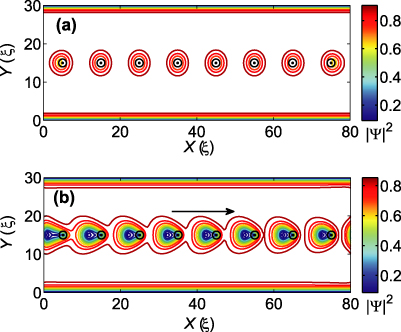
Figure 4. (a) The vortex structure at the initial state (without a driving current). (b) A snapshot of moving antivortices in the film with parallel magnetic dipoles (indicated by black circles with dots in the middle). All antivortices move in one direction indicated by the arrow. The magnetic dipole moment is μ = 1μ0 and the height z = 2.8ξ above the SC.
Download figure:
Standard imageWhen the magnetic moment is larger than μ0 and there are satellite vortices, the v–av dynamics becomes more complicated. Vortices and antivortices move and annihilate in between the dipoles. At a current magnitude of 0.25j0, the satellite vortices move slower than the vortices that hop between the pinning sites. With a further increase of the transport current, e.g., for j = 0.3j0, the flux flow occurs mainly via the 'channel' with pinning sites. For the opposite polarity of the dipoles, the flow direction is reversed. This is due to the fact that vortices turn to antivortices and vice versa. The direction of the vortex (and, correspondingly, antivortex) motion will be opposite.
When we change the distance a from 7.5ξ to 10ξ between the dipoles, we observe a change in the IV curve (figure 5). Thus increasing a results in an increase of the critical current from 0.23j0 to 0.285j0. This increase of jc can be explained as follows. The magnetic field of the dipoles depletes the order parameter under the dipoles. This local inhomogeneity of the order parameter serves as a vortex nucleation point. This suppressed order parameter region pins free vortices. Placing dipoles close to each other we create a 'channel' (rather than a chain of separate localized minima) of depleted order parameter regions. Therefore, the dipoles that are closer to each other lead to an enhanced motion of the vortex from one pinning center to the other. It means that their mobility (along the row of the pinning centers) increases [13]. In the limit when the order parameter minima merge, the vortices move along the 'path of the depleted order parameter'. Due to the merging of the depleted order parameter regions, the critical current is smaller for closely located dipoles and drops to zero when the 'pinning sites' are close enough [13].
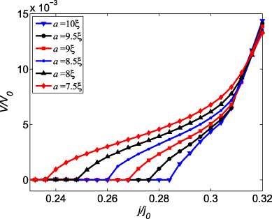
Figure 5. The IV-curves for various distances a between the magnetic bars with μ = 1μ0 and z = 2.8ξ.
Download figure:
Standard imageTherefore, the above analysis of the order parameter distribution and the IV-curves allows us to gain insight into the v–av dynamics of the system and to understand the observed dependence of the critical current jc on the geometry of the system.
4.2. Antiparallel array
An antiparallel configuration of bars is shown in figure 1(a). The direction of the magnetic field near the tips of the neighboring bars is opposite and we do not find any satellite vortices for various μ. This is explained by the fact that the antisymmetric field distribution in the vicinity of the bars mutually cancel out for any value of the magnetization μ (figure 3(b)). In the presence of the transport current, vortices move in the middle of the film.
In this regime, the flux carrying mechanism is different from the previous one and, as a result, the v–av dynamics becomes much more complicated. Under each tip of a magnetic bar, a vortex and an antivortex are generated. A vortex of one out-of-plane (up) dipole tends to annihilate with an antivortex of another out-of-plane (down) dipole. However, there are also an antivortex left under the out-of-plane (up) dipole and a vortex under another (down) dipole. They annihilate in the neighbor unit of the dipole chain. Each unit contains regions under two neighboring tips, as shown in figure 6 by solid and dashed boxes. Vortex–antivortex annihilation occurs first in the central unit (solid box), then in two neighbor units (dashed boxes) and so on (toward the film boundary). This v–av dynamics includes two phases: the first one is the annihilation of v–av pairs in the solid boxes and the second in the dashed boxes, then the process repeats periodically. The v–av creation and annihilation dynamics can be presented as a subsequent alternation of the phases shown in figures 6(b) and (c). The (anti)vortices annihilate in the central unit, then they annihilate between neighbor dipoles of another unit (as a 'chain'), then the process repeats. This v–av repeating process results in two directed flows: vortex flow from the left to the right and antivortex flow from the right to the left.
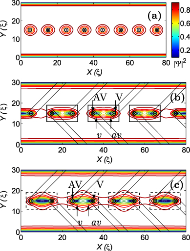
Figure 6. Snapshots of the square modulus of the order parameter at 50 τGL, illustrating the vortex dynamics in the film with antiparallel dipoles. The equilibrium state (a): no vortex motion. The circled dots and circled crosses show the direction of the magnetic dipoles at the bar tips. The symbols v,av show the vortices and antivortices that move and annihilate, while V,AV mark the remaining vortex/antivortex. The panels (b) and (c) show two characteristic regimes of the annihilation between neighboring out-of-plane dipoles.
Download figure:
Standard imageWe have examined the influence of the length of the system on the critical current jc. We found that if we change the distance between the dipoles, and keep the length of the film constant, then the critical current will be changed. The IV-curve for an antiparallel dipole chain reveals a larger critical current than that for the parallel dipole configuration. The strength of 'pinning' of (anti)vortices is defined by the depth of the magnetic-field profile. This is explained by different potential profiles induced by parallel and antiparallel out-of-plane dipoles. Clearly the pinning strength is larger in the case of AP dipoles and, therefore, antiparallel arrays of dipoles trap vortices more strongly. The critical current and the IV-curve depends on the profile of the dipole magnetic field. The broader the profile of the dipole magnetic field, the lower the critical current. The v–av dynamics is also strongly affected by this profile. One can see this difference in figure 7: different curves correspond to various dipole magnetic moment and separation z. One can clearly distinguish flux flow and pinned regimes when analyzing the IV-curves shown in figure 7. The weak and low out-of-plane dipole (i.e., for small z) facilitates the pinned regime and results in larger critical currents. Despite the fact that the magnetization of the dipoles is weak, their magnetic field is localized and results in narrow pinning centers. A strong dipole with a large z is characterized by a broad profile and favors the flux-flow regime: the region of depleted order parameters is large and the vortex is therefore not localized. This gives rise to a large vortex mobility, which in turn results in a flux-flow regime.

Figure 7. (a) The IV-curves for an antiparallel dipole chain for: μ = 1μ0, z = 1z0; μ = 8μ0, z = 2z0; μ = 64μ0, z = 4z0. The critical currents jc (shown by small arrows) are: 0.276j0, 0.077j0, 0.0j0 correspondingly. (b) The IV-curve for the parallel dipole chain. The critical currents jc are: 0.039j0, 0.026j0, 10−4j0 correspondingly. Here μo = 5.6Φ0ξ/8π and z0 = 2.8ξ.
Download figure:
Standard imageWe have shown that depending on the initial magnetization, the critical current varies in a broad range of jc (see figure 7). It is interesting and desirable, from the point of view of possible applications, to optimize the critical current jc and thus the performance of our device, i.e., the ratio between the critical current for parallel and antiparallel configurations.
Now we will focus on the selection of the system with the highest critical current in the flux-flow and flux-pinned regimes. Optimization includes finding a system with the largest ratio of the critical currents. For this purpose, we introduce the 'quality-factor' of the pinning array, i.e., the ratio of the critical current in the pinned regime (AP configuration), to that in the flux-flow regime (P configuration),  of the system which is plotted in figure 8 versus the distance a between the rows of parallel bar (see figure 1). The ratio between the critical current in the pinned and flux-flow regime depends on the distance between the magnetic bars a and on the magnetic field produced by the bars. The magnetic-field profile of the bar depends on the ratio of the bar magnetization to the height of the bar above the SC surface. We discussed these parameters in section 3. Figure 8 shows that the ratio
  changes with varying distance between the bars: it reaches a maximum value for some bar magnetization (μ = 1μ0 and z = 2.8ξ) or diverges (for
  ). This is due to the significant critical current drop (in the flux-flow regime) which happens for large magnetization values. However, the critical current (in the pinned regime) remains the same, but the ratio of these critical currents increases.

Figure 8. The ratio of critical currents in the flux-flow and pinned regimes  , versus the distance a between the rows of parallel magnetic bars. The legend shows the magnetization of the bars and its height above the SC, z.
Download figure:
Standard image5. An array of wide magnetic bars
In this section, we consider an array of magnetic bars of finite width. The latter means that it is no longer possible to model the bars by out-of-plane dipoles, and we calculate the magnetic-field profile of the in-plane bars. On the other hand, it is clear that it is the out-of-plane component of the magnetization that is responsible for the generation of (anti)vortices and their 'pinning'. However, in this case the regions of suppressed order parameter become rather extended, as compared to the case of narrow bars. A typical bar arrangement with separation parameters Dx,Dy is shown in figure 9. The modeled in-plane magnetized bars are shown by black and red (gray) dotted areas. Each bar is modeled by 96 elementary in-plane magnetized dipoles. This corresponds to the sizes: length ≈ 22ξ, width ≈ 4.2ξ.
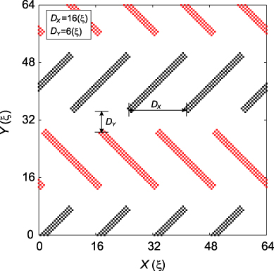
Figure 9. One of the typical magnetic bar configurations. The distances between the bars in the x- and y-directions are Dx = 16ξ and Dy = 6ξ, correspondingly. The sizes of the bars are: length ≈ 22ξ, width ≈ 4.2ξ.
Download figure:
Standard imageThe order parameter plots and the corresponding bar configurations are shown in the insets of figure 10 for the P and AP configurations. The magnetic field outside the SC film area is also taken into account. This magnetic field influences the (anti)vortices in the film. It turns out that there are less vortices for the AP configuration than for the P configuration in the film for the same bar configuration, resulting in a smaller resistance and larger critical current.

Figure 10. The IV-curves for the parallel (P) and the antiparallel (AP) dipole configurations. The insets show snapshots of the order parameter in the stationary dynamic regime for the AP (right bottom) and P (left top) magnetic configuration, for j/j0 = 0.21 (P) and j/j0 = 0.31 (AP). The modeled bars are shown by black and red (gray) dotted areas.
Download figure:
Standard imageIt was found that for relatively large distances between the magnetic bars, a vortex attached to one magnetic bar annihilates with an antivortex of the neighboring bar. There is no v–av motion present between the rows, but only inside the rows. For small spacing between the bars, the situation is more complicated: the trajectories of motion of vortices and antivortices overlap and it is difficult to distinguish vortex (antivortex) cores in order to investigate their dynamics.
In figure 11 we show a set of the IV-curves for parallel (a) and antiparallel (b) bar magnetization for varying distance Dx between the bars. The main feature of the IV-curves is that the critical current for the AP configuration is larger than that for the P configuration, for the same Dx and Dy. This result is in agreement with recent experimental results [23]. However, the ratio  , which is the measure of the difference between the critical current in AP and P configurations, can be further improved through the adjustment of the distance between the bars on the film surface in the xy-plane.

Figure 11. The IV-curves for parallel (a) and antiparallel (b) configurations. The distance between the bar centers is presented in the legend and Dy = 4ξ.
Download figure:
Standard image5.1. Critical current behavior in the parallel configuration
Our calculations show that with increasing separation between bars either in the x-direction, Dx, or in the y-direction, Dy, the critical current in the P configuration increases monotonically (see figures 11(a) and 12). When Dx increases (and Dy is constant), the area of unperturbed order parameter is enlarged. This can be easily understood intuitively: for smaller density of pinning centers the order parameter in the film is less suppressed by the magnetic field, and (anti)vortices cannot easily jump from one pinning center to another one. This leads to an increase in jc.

Figure 12. The critical current  and
and  as function of the distance between the magnetic bars Dx (Dy = 4ξ).
Download figure:
Standard imageIncreasing Dy, while keeping Dx constant, also leads to an increase of the critical current. However, for large enough Dy (Dy > 10ξ), vortices will move along two independent rows of pinning sites (separated by Dy), and a further increase of Dy will not influence the v–av dynamics and jc.
Analyzing the behavior of the critical current jc when simultaneously changing Dx and Dy, we found that jc can be effectively controlled in this device. Figure 13 shows typical IV-curves for varying Dx and Dy. One can see from this plot that the difference in the critical currents for P and AP configurations can be controlled in a broad range, from an order of magnitude difference (figure 13(a)) to zero (figure 13(c)).

Figure 13. The IV-curves for parallel (P) and antiparallel (AP) dipole configurations. The distance between the bar centers is (a) Dx = 4ξ,Dy = 0ξ; (b) Dx = 6ξ and Dy = 4ξ; (c) Dx = 7ξ, Dy = 0ξ.
Download figure:
Standard image5.2. Critical current behavior in the antiparallel configuration
The dependence of the critical current on the distance between the bars for the AP configuration is more complex than that for the P configuration. The magnetic fields of the neighboring bars cancel each other partially for small Dx and Dy. While the critical current as a function of Dx still increases for Dx > 7ξ, similarly to the case of the P configuration, it shows a non-monotonic behavior for small Dx (see figure 12). The revealed increase of jc for small Dx in the AP configuration is due to the annihilation of v–av pairs for strongly overlapping magnetic profiles of opposite polarity (see also [33]).
Increasing the separation between the pinning sites in the x-direction (Dx) leads to an increase of the depth of the magnetic-field profile, due to the decreasing overlap between the local magnetic fields of opposite polarity created by the magnetic bars. As a result, the critical current jc as a function of Dx increases for 7ξ < Dx < 12ξ (see figure 12). For even larger Dx, the depth of the magnetic-field profile does not change and the function  saturates (see figure 12).
Using the obtained results for the critical current for the P and AP configurations we have also analyzed the ratio  in the plane (DxDy). The result is shown in figure 14. The maximal value of
  is reached for closely spaced bars. For other limiting cases (small Dx and large Dy; large Dx and small Dy; large Dy and large Dx) the ratio
  tends to unity.

Figure 14. The map of the ratio  as a function of the distances between the magnetic bars.
Download figure:
Standard imageThis result ( ) can be understood in the case of well-separated bars (e.g., Dx > 6ξ and Dy > 4.5ξ). Due to the fact that the vortex (antivortex) paths do not overlap for large Dy (see figure 15), there are equal numbers of (anti)vortex paths in the long (in the y-direction) film with either P or AP configuration. The difference in the vortex flows of the AP and P configurations is situated in the vortex and antivortex flows in the neighboring paths: in one configuration (P) there are moving vortices in both paths and in the other configuration (AP) there are vortices in one path and antivortices in the other. Therefore, in the AP configuration there are two counter-flows in neighboring paths: one consisting of vortices and another one of antivortices. The number of moving vortices and antivortices in every path is equal. It means that the counter-flow in one path generates an equal voltage as the flow in neighboring paths. It is clear that the critical currents of these two configurations will be the same.

Figure 15. Two nearest vortex (antivortex) paths in AP and P configurations. It illustrates the equal critical currents for the two configurations in a long (in the y-direction) film.
Download figure:
Standard image6. Conclusions
Using the time-dependent Ginzburg–Landau equations, we have investigated the vortex–antivortex dynamics in a hybrid system consisting of a superconducting film with an array of magnetic bars on top, as was recently realized experimentally in [22, 23]. In the plane of the film, the magnetic bars form parallel rows of bars oriented perpendicular with respect to the bars in the adjacent row, i.e., they are arranged in a 'zigzag' configuration.
The striking property of this zigzag array is that, by changing the magnetization of the magnetic bars by applying an in-plane magnetic field, the configuration of the magnetic field can be switched from 'parallel' to 'antiparallel', i.e., when the apices of the neighboring bars in the rows are magnetized either in the same or in the opposite direction. This switch of the magnetic-field configuration has a dramatic impact on the dynamics of the vortex–antivortex motion in the system and the mechanism of the flux transfer. We consequently simulated the system with out-of-plane dipoles (i.e., for narrow bars) and in-plane dipoles (for wider bars). The results are consistent with each other and lead to the same conclusions. The parallel configuration is characterized by a dense and shallow potential profile which favors the flux-flow regime having low critical currents. Contrary to that, the antiparallel configuration is characterized by a relatively deep and less dense potential profile resulting in a flux-pinned regime with a high critical current. While this main result is easily understandable, and our results agree with recent experimental observations in [22, 23], the mechanisms behind the flux transfer and the detailed vortex–antivortex dynamics is rather complicated in this system. As we demonstrated, it involves the process of vortex–antivortex generation under the tips of the bars (or in the vicinity to the bars) and their annihilation, which is strongly affected by system parameters such as the magnetization of the bars, the spacing between the bars in the plane of the superconductor and the spacing between the bars and the superconductor. Using the results of calculations and understanding the different underlying mechanisms of flux transfer, one can improve the performance of this artificial device, i.e., to increase the ratio of the critical currents for the two distinct in-plane magnetizations: parallel and antiparallel,  , by using zigzag-arranged magnetic bars, which can be useful for magnetic flux manipulation in fluxonics applications.
Acknowledgments
We acknowledge useful discussions with Denis Vodolazov and Alejandro Silhanek. This work was supported by the 'Odysseus' Program of the Flemish Government and the Flemish Science Foundation (FWO-Vl).