
Abstract
Identifying radon-prone areas is key to policies on the control of this environmental carcinogen. In the current paper, we present the methodology followed to delineate radon-prone areas in Spain. It combines information from indoor radon measurements with γ-radiation and geological maps. The advantage of the proposed approach is that it lessens the requirement for a high density of measurements by making use of commonly available information. It can be applied for an initial definition of radon-prone areas in countries committed to introducing a national radon policy or to improving existing radon maps in low population regions.
Export citation and abstract BibTeX RIS

Content from this work may be used under the terms of the Creative Commons Attribution 3.0 licence. Any further distribution of this work must maintain attribution to the author(s) and the title of the work, journal citation and DOI.
1. Introduction
Radon (222Rn) exposure indoors is recognised by the World Health Organization as the second most important cause of lung cancer in many countries. The main authorities in the radiological protection field have strengthened radon provisions in their principles or standards (ICRP 2009, IAEA 2011, EC 2012), driven to some extent by the epidemiological evidence made available from radon domestic exposure studies (Darby et al 2005, Krewski et al 2006, Lubin et al 2004). In Europe, for example, radon exposure in the home has been estimated to account for over 9% of all lung cancer deaths (Darby et al 2006).
From a national public health perspective, the magnitude of the radon problem largely depends on geology, specifically on the 226Ra content and the permeability of the rock formation. Other factors that play an important role include the construction methods of buildings, and the climate.
A strategy to control radon exposure should address the whole population, both at home and in the workplace, while devoting special efforts and resources to the individuals most at risk, namely those with exposures in the right tail of the lognormal distribution that typically describes radon indoor concentrations. A very high radon level can be found in a building regardless of its location, but certain areas are much more prone to give rise to high concentrations in dwellings. Consequently, the identification of such areas is a key issue in an effective regulatory control of radon exposure.
There is no consensus definition of a radon-prone area. Generically, the 2007 Recommendations of the ICRP define it as an area in which the concentration of radon in buildings is likely to be higher than the national average. In some countries, this definition is based on a given fraction of dwellings exceeding a regulatory reference level.
The most straightforward method to delineate radon-prone areas is based on actual in-house radon measurements (see, for instance, Miles 1997, Andersen et al 2001, Friedmann 2012). Because it requires a relatively large number of indoor radon measurements and a sampling density that is representative of the building stock, this method is only achievable nationwide when a significant fraction of all dwellings across the country has been monitored for radon.
An alternative to map radon hazard is to measure radon in soil gas. This is a good predictor of indoor radon because soil usually is by far the main entry path of radon into buildings (Nazaroff et al 1988). Both the Swedish and the German systems are based on the assessment of geogenic radon potential, which is derived from soil gas measurements at one metre depth and soil permeability (Åkerblom 1986, Kemski et al 2001).
Other indirect methods are based on the positive correlation of 238U or 226Ra concentration in surface rock or soils with radon in soil gas (Agard and Gundersen 1992), and, in turn, with radon in dwellings. Ielsch et al (2010) mapped the geogenic radon potential in Bourgogne (France), applying a classification scheme of geological units according to their uranium content determined by means of rock sample analysis. The suitability of equivalent uranium (eU) derived from airborne surveys of γ-rays to map radon-prone areas has also been demonstrated in regions of Canada, Northern Ireland and Norway (Ford et al 2000, Appleton et al 2011, Smethurst et al 2008). In addition, the US EPA map of radon zones (US EPA 2013) includes aerial radiometric data on eU as one of the factors contributing to radon potential in a given area.
In Spain, although several regional surveys have identified areas of high radon exposure (Matarranz 2004), a nationwide delineation of radon-prone areas cannot be achieved by analysis of the in-house radon measurements alone because these present gaps in spatial coverage and are insufficient in number compared to the housing stock.
However, such areas need to be identified throughout the country, applying a uniform methodology, in order to prompt legislative action aimed at reducing the exposures of people residing in risk areas. As radon regulation is enacted at national level, it would be unacceptable to create regulation that is binding in some parts of the territory while setting aside other areas that are subject to similar or greater risk. In addition, it would be advantageous to delineate radon-prone areas at the smallest administrative level (which in Spain is the municipal one) since this would allow for a better use of public resources and a more efficient distribution of regulatory burdens.
In this paper, we present a methodology to map areas countrywide where 10% of residential buildings and houses exceed the reference level of 300 Bq m−3 set in national legislation (CSN 2011). This methodology makes use of the current radon measurement database and other available surrogate information, including the natural γ radiation map of Spain at 1:1000 000 scale (Suárez et al 2000). We show that outdoor γ-ray exposure at 1 m above ground can contribute to successfully delineate radon-prone areas. We choose an outdoor absorbed dose rate in air of 66 nGy h−1 as the cut-off point below which municipalities are considered non-radon-prone. Above this value, we take into account geological information and group radon measurements by lithostratigraphic unit. Each of these units is classified as radon prone or non-radon-prone based on a hypothesis test on the 90th percentile for the corresponding distribution of radon levels.
The method is proven to work well over a surface of about 500 000 km2 (mainland Spain) of very diverse geology and precipitation regime, ranging on average from less than 300 mm yr−1 in the southeast to more than 2000 mm yr−1 on the northern coast.
2. Input data
In order to produce the map of radon-prone areas, we merged the following data sources using ESRI ArcGis v. 10.0 (ESRI 2011):
- The national indoor radon database.
- The natural γ-radiation map.
- Geological (lithostratigraphic and metallogenic) maps.
2.1. Indoor radon database
The national radon database currently has over 11 000 records of in-house radon measurements grouped by municipality. Several research groups have contributed to the database (Quindós et al 1991, Gutiérrez et al 1992, Amorós et al 1995, Baixeras et al 1996, Pérez et al 1996, Baeza et al 2003, Quindós et al 2011), the bulk of measurements having been collected by the University of Cantabria through different projects sponsored by CSN. The resulting sampling density is spatially heterogeneous, tending to be higher in regions with elevated radon level and at the most densely populated areas.
Roughly 90% of measurements were made with solid-state nuclear track detectors exposed for a period from three to six months, whereas the remaining 10% were obtained with charcoal canisters exposed over three days. Although, on a house-by-house basis, short-term measurements do not provide as reliable estimates of the annual radon level as the several-month-long measurements, an overall good agreement was found in surveys conducted in all municipalities where the two types of result could be compared (García-Talavera et al 2013). Furthermore, because our scope was to quantify risk rather than actual population exposure, we selected measurements made at ground or first floors.
The current radon database suffers from some limitations that hamper modelling approaches: it neither reports precise measurement location (only name of the village, town or city is provided) nor contains information on relevant dwelling characteristics (such as year of construction or type of foundation). Moreover, there are a limited number of measurements in comparison to the building stock. Out of the approximately 7900 municipalities in peninsular Spain, radon measurements have been made in 1170. Yet, for roughly one-third of them, the number of available measurements (n) is 1 or 2; 452 have 7 ≤ n < 26; and 25 have n ≥ 27.
2.2. The natural γ-radiation map
Many countries have developed γ-radiation maps of their territories, as such maps are cost effective and have manifold applications: information on population radiation doses, documented baseline for accident and emergency situations, aid to raw materials or mineral exploration, etc.
The MARNA (Map of Natural Radiation of Spain) was undertaken as a collaborative project of CSN and ENUSA and joined later by several universities (Suárez et al 2000). Its main objective was to draw up a map of natural γ-radiation expressed as microroentgens per hour (μR h−1) at 1 m above ground.
It combined information from various sources.
- Over 150 000 aerial measurements from uranium deposit exploration obtained in radiometric flights at an altitude of 120 m between 1967 and 1981. The detectors used were large volume NaI scintillators with an energy window from 0.4 to 2.8 MeV.
- Ground-based measurements, static and car-borne, also obtained in uranium exploration campaigns covering an energy window from 0.4 to 2.8 MeV.
- Over 450 000 ground-based static and car-borne measurements from project-specific campaigns using Saphimo SRAT and ES3 S equipment for total counting and an Exploranium GR-1300 for spectrometric measurements.
After correcting the airborne data for cosmic radiation, a good agreement was found between airborne and ground measurements (linear correlation coefficient greater than 0.92). To draw up the map to 1:1000 000 scale, mean radiometric values (corresponding to a nominal cell size of 7 km×5 km) were used. The 7 km×5 km grid of regularly spaced values was submitted to a kriging interpolation using Golden Software Surfer 7. In this step, an anisotropic variogram model was specified whose parameters were locally varied to describe the orientation of geological structures. The performance of the kriging model was verified by standard cross-validation.
2.3. Geological maps
Lithostratigraphic (LS) information was extracted from the 1:200 000-scale national map developed by the Institute of Geology and Mineral Exploration (IGME 2012a). This map represents cartographic units that are delimited mainly on the basis of lithic characteristics and stratigraphic position.
The metallogenic map at 1:200 000 scale (IGME 2012b) showing the nature and distribution of mineral resources was used to establish the location of uranium deposits and occurrences. The most important of the several tens of known uranium mineralised zones are located in the Schist–Greywacke Complex, a geological structure of the Central Iberian Hercynian belt. They mainly occur in fracture and breccia zones of Palaeozoic slates and granitic plutons.
3. Statistical framework
We classify an area as radon prone when the 90th percentile of indoor radon concentration in its building stock is greater than the reference level. In practice, nevertheless, classification has to be done under uncertainty, as only a small sample of the dwellings in an area would typically have been measured for radon and, consequently, the point estimate of the percentile would differ from the true value of the population percentile.
There are many ways of calculating percentiles, but, given that the shape of the distribution is known, a parametric estimate would in principle be subject to less error. Because radon measurements in dwellings most often conform to a lognormal distribution, the parametric estimate is usually preferred. For a lognormal distribution, this can be obtained as a function of the sample geometric mean and the sample geometric standard deviation. If the geometric standard deviations of the areas in question do not differ statistically, the geometric means can be used instead of the percentiles for area classification.
Point estimates, however, do not provide a piece of information that hypothesis testing does: whether there are significant differences between the true value of a parameter and its estimate. Therefore, the most consistent approach to area classification is to acknowledge uncertainty by basing the decision on a statistical hypothesis test. Specifically, we have developed a hypothesis test that uses the upper bound on the 90th percentile as the critical value.
As for the rest of statistical tests included in this paper, we have used SPSS v. 19.0 (IBM Corp 2010) and the R software (R Development Core Team 2008).
3.1. The radon-prone hypothesis test
If we denote by X0.9 the 90th percentile of indoor radon concentration, X, in a given area, the problem of classifying it as radon prone or not can be formalised as a hypothesis test problem where the null hypothesis, H0: X0.9 ≥ 300 Bq m−3, is tested against the alternative hypothesis, H1: X0.9 < 300 Bq m−3. The critical point for rejecting H0 is  , the upper bound on X0.9, at the α-significance level.
As it is customary, we assume that indoor radon data, X, follow a lognormal distribution. We denote by mg the sample geometric mean and by sg the sample standard geometric deviation. Then, the random variable Y = logX is normally distributed with mean μy and standard deviation σy.
Given a random sample {xi}, the upper bound on the 90th percentile of Y, Y0.9, can be obtained as (Hahn and Meeker 2011)

where  is the sample mean of {yi} = {logxi},
  , n is the sample size, sy is the standard deviation of {yi}, and the factors
  are given in table 1 of Odeh and Owen (1980).
Because of the relationship between the theoretical percentiles of X and Y, P{Y < Y0.9} = 0.9↔P{X < eY0.9} = 0.9, the upper bound on the 90th percentile of X is
At the α-significance level, the null hypothesis can be rejected (thus concluding that a particular area is not radon prone) if and only if  . In particular, we set α = 0.10 (probability of type-I error), which allows for a 10% probability of failing to identify a true radon-prone area.
The above equation can be applied for n > 2, but small sample sizes would result in large probabilities of type II error (incorrect non-rejections of H0). To control this effect, Faulkenberry and Weeks (1968), suggested that the sample size be large enough so that
- (i)there is a large probability (1 − α) that the tolerance bound will be exceeded by at least 100p'% of the normal population, and
- (ii)the probability (δ) that more than 100p*% of the population will exceed the said tolerance bound is small, where p' and p* are specified proportions, and p* > p'.
The probability of a successful demonstration is pDEM = Pr(p > p') ≥ 1 − δ. For p' = 0.90; p* = 0.98 and δ = 0.10, we get a minimum sample size of 27. Consequently, we established this figure as the minimum sample size to apply the radon-prone hypothesis test.
4. Results and discussion
Delineating radon-prone areas at municipal level requires data on the probability of exceeding the radon reference level for every municipality in the country. Such a probability, however, cannot be based on in-house measurements alone, since these are only available at a small percentage of municipalities, with barely a few tens of them reaching the minimum sample size established to apply the radon-prone hypothesis test.
Hence it was necessary to identify whether, on a country-size scale, other environmental variables might be good surrogates for indoor radon so as to make reasonably accurate predictions at unsampled or poorly sampled locations. Specifically, we investigated outdoor γ-dose rate and geology.
4.1. Modelling indoor radon as a function of γ-dose rate
Previous research (Cascón et al 2002) had shown that γ-dose rate across the country exhibits a linear relationship with 226Ra in soil, which, in turn, is known to be correlated with 222Rn indoors (Nason and Cohen 1980). This fact prompted a study on the usability of the γ-radiation map of Spain to predict radon levels directly in a northwestern granitic region (Quindós et al 2008). Three areas with different γ-radiation levels (<65–87 nGy h−1, 65–130 nGy h−1, and 87–>130 nGy h−1) were measured for radon indoors. Based on the main statistical parameters for the three corresponding radon distributions, this study concluded that γ-radiation dose rate is a qualitative indicator of high indoor radon level rather than a good quantitative predictor.
We analysed the relationship between indoor radon concentration and γ-dose rate using data from the whole Spanish mainland. In particular, for each municipality, we considered the geometric mean (mg) and the geometric standard deviation (sg) of the measured radon concentrations, provided that there were more than six available measurements3. The corresponding average γ-dose rate was obtained from the MARNA map as follows: the built-up area of the municipality was determined using information provided by the National Centre for Geographic Information in a 1 km × 1 km grid. By a bilinear interpolation from the MARNA surfaces, the program Surfer 7 provided the γ-exposure value at the centre of every grid cell over which the built-up area spreads. We then computed the average of these values and converted it to absorbed dose in air using 1 R =0.008 76 Gy.
Our analysis showed that there is a statistically significant but rather weak correlation between radon geometric mean (GM) and average γ-dose rate (Rγ): Pearson r = 0.30, p = 0.001; Spearman ρ = 0.65, p = 0.000.
Radon geometric standard deviation (GSD), on the other hand, is not linearly correlated either to GM (r = 0.087; p = 0.082) or to Rγ (r =− 0.060; p = 0.229), although it exhibits a weak but significant rank correlation with the former variable (ρ = 0.108, p = 0.030). The distribution of GSD for all municipalities with n > 6 has a median value of 2.05, and a range going from 1.13 to 6.93.
The natural logarithm of GM is better correlated with Rγ (r = 0.61; p = 0.000). We performed a minimum least-squares analysis for Rγ versus ln(GM) (see figure 1), obtaining an R2 value of 0.37. A very poor fit (R2 = 0.05) was achieved when, instead of geometric means, 90th percentiles (X0.9), assessed by the maximum likelihood parametric estimate, were considered.
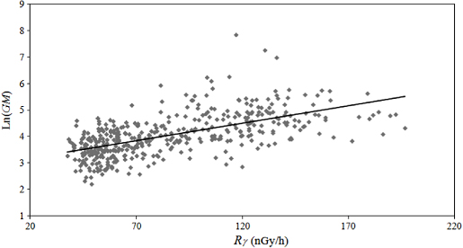
Figure 1. Linear least-squares regression fit for average γ-dose rate (Rγ) in nGy h−1 and natural log of geometric mean (GM) of radon concentrations in Bq m−3.
Download figure:
Standard image High-resolution imageNone of these regression models can explain a sufficient amount of variation to allow the construction of radon maps that carry an acceptable confidence of accuracy. Yet the relevant information to label an area as radon prone is not actually mg nor X0.9, but the probability of them exceeding a certain threshold value. This means that, to this purpose, radon indoors can be expressed as a categorical rather than as a quantitative variable, as presented in section 4.2.
4.2. Correspondence between categorical variables
First, we investigated the role of γ-dose rate as a categorical variable using the same dataset as in section 4.1: we selected cut-offs of 66 nGy h−1 (∼7.5 μR h−1) and 123 nGy h−1 (∼14.0 μR h−1) for the γ-dose rate because the categories defined by these values provide a good division of geological units (the >7.5 μR h−1 surface roughly corresponds to the Pre-Mesozoic geological setting of peninsular Spain, whereas the 14.0 μR h−1 contour line encloses some granitic outcrops and westernmost distinct metamorphic areas of the Iberian Massif—see figure 4).
We considered the distribution of radon geometric means for each group of municipalities defined according to the γ-dose rate categories established above (see box plot in figure 2). The three of them can be described by a lognormal distribution (Kolmogorov–Smirnov test: Z0 = 0.514; p0 = 0.954; Z1 = 1.161; p1 = 0.135; Z2 = 1.089; p2 = 0.186). Levene's test, performed on the log-transformed data, showed heterogeneous variances (W = 5.303; p = 0.005). Thus, we applied the Kruskal–Wallis test, which revealed that the three groups are statistically different (χ2 = 151.4; p < 0.05).
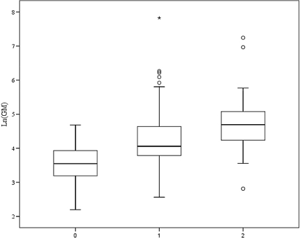
Figure 2. Box plot of natural log of radon geometric mean for municipalities subjected to the following average γ-dose rates: (0) <66 nGy h−1; (1) 66–123 nGy h−1; (2) >123 nGy h−1.
Download figure:
Standard image High-resolution imageNext we carried out a correspondence analysis to explore the degree of association between the following categories of γ-dose rate and indoor radon (GM).
- <66 nGy h−1 and <70 Bq m−3.
- 66–123 nGy h−1 and 70–120 Bq m−3.
- >123 nGy h−1 and >120 Bq m−3.
A good association was found for the three pairs (see figure 3(a)). Figure 3(b) shows a graphic representation of the associated contingency table. A geometric mean of 70 Bq m−3 corresponds (for n = 27 and sg = 2.37, namely, the 75th percentile for the GSD distribution) to a 90% confidence upper bound on X0.9 of approximately 300 Bq m−3. The 120 Bq m−3 cut-off was selected because it achieves the closest association to the >123 nGy h−1 category.

Figure 3. (a) Two-dimensional correspondence map showing a close association between the following categories of γ-dose rate and radon concentration: <66 nGy h−1 and <70 Bq m−3; 66–123 nGy h−1 and 70–120 Bq m−3; >123 nGy h−1 and >120 Bq m−3. (b) Segmented bar chart representing the relationship between Rγ and GM. It compares the percentage (and number of cases) that each radon category contributes to a total across categories of Rγ.
Download figure:
Standard image High-resolution imageOut of 181 municipalities with average γ-dose rate < 66 nGy h−1, nearly 90% (95% CI=(0.85,0.94) estimated by the modified Wald method; Agresti and Coull 1998) have radon geometric means lower than 70 Bq m−3. A higher proportion, 97% (95% CI=(0.93,0.99), likewise calculated), have 90th percentiles lower than 300 Bq m−3.
Therefore, selecting a cut-off point of 66 nGy h−1 for a screening test based on γ-dose rate can be a valid option to discriminate non-radon-prone municipalities. We considered two such screening tests using the following criteria, respectively, to define radon-prone areas: (i) mg ≥ 70 Bq m−3; (ii) X0.9 ≥ 300 Bq m−3. Table 1 shows their positive predictive value (PPV, probability that a municipality is radon prone given that the test result is positive) and their negative predictive value (NPV, probability that the municipality is non-radon-prone given that the test result is negative). Both tests have a poor PPV but achieve a high NPV, notably for X0.9.
Table 1. Positive predictive value (PPV) and negative predictive value (NPV) of a test with a cut-off point of 66 nGy h−1 γ-dose rate for screening municipalities with radon mg ≥ 70 Bq m−3 and municipalities with radon X90 ≥ 300 Bq m−3.
| PPV | NPV | |
|---|---|---|
| mg ≥ 70 Bq m−3 | 0.54 | 0.90 |
| X90 ≥ 300 Bq m−3 | 0.25 | 0.97 |
Because of the high NPV, regardless of the selected point estimate, all areas with γ-dose rate lower than 66 nGy h−1 (∼7.5 μR h−1) were directly classified as non-radon-prone—see map in figure 4. Most of these correspond to Tertiary and Quaternary soils developed over calcareous sedimentary rocks.

Figure 4. Map of γ-ray exposure at one metre above the ground (Rγ) for mainland Spain. Blank areas are directly classified as non-radon-prone.
Download figure:
Standard image High-resolution imageConversely, for areas with γ-dose rate in excess of 66 nGy h−1, γ-radiation does not exhibit a strong enough control on radon indoors to make a reliable classification (see the first two bars in figure 3(b)). Even the highest γ-dose category contains a significant proportion (∼20%) of non-radon-prone municipalities.
4.3. Merging geological information
The control of geology on indoor radon levels is well recognised (Miles and Ball 1996, Mikšová and Barnet 2002, Kemski et al 2002, Appleton and Miles 2010, Friedmann and Gröller 2010). Consequently, for those parts of the country with γ-dose rate in excess of 66 nGy h−1 (i.e., >7.5 μR h−1 surface from map in figure 4), we included geological information in the analysis in order to establish radon-prone areas at geological-formation level rather than at municipality level. Specifically, we considered the lithostratigraphic (LS) map of Spain.
To analyse radon data, we selected all LS units that intersected in more than 10% of their surface with populated regions exhibiting γ-dose rate >66 nGy h−1. Some of these units were further regrouped based on composition, age and permeability (see table 2). The LS unit has, on the one hand, a characteristic range of 226Ra concentration and, on the other hand, a typical permeability4 value, both of which have a link to indoor radon. Yet, even within the same LS type, a substantial variability of indoor radon levels could be found due to the influence of unaccounted-for variables (such as climate, dwelling characteristics, or depth to the water table).
Table 2.
Statistical parameters of radon levels and average γ-dose rate ( ) in lithostratigraphic units within regions of γ-dose rate values predominantly higher than 66 nGy h−1. Those whose upper bound on the 90th percentile (
 ) of measured radon concentrations exceeds 300 Bq m−3 are classified as radon prone.
| Unit description | Sample size |
 (nGy h−1) (nGy h−1) |
mg(Bq m−3) | sg |
 (Bq m−3) (Bq m−3) |
|---|---|---|---|---|---|
| Hercynian acid plutonic rocks (Palaeozoic) | 770 | 131 | 118.0 | 2.7 | 452.5 |
| Hercynian arkosic sandstone and schist (Palaeozoic) | 96 | 121 | 57.6 | 2.8 | 261.9 |
| Sedimentary deposits of Tertiary age (Guadiana basin) | 164 | 117 | 55.7 | 1.8 | 130.9 |
| Slates, metagraywacke and mica-schist (Precambrian–Palaeozoic) | 331 | 114 | 98.0 | 2.7 | 375.4 |
| Metamorphic rocks (Precambrian–Cambrian–Ordovician) | 85 | 110 | 131.9 | 2.3 | 459.6 |
| Tertiary siliciclastic deposits, mainly arkosic sandstone and mudstone (Tagus–intra-Betic–Guadalquivir) | 131 | 110 | 70.1 | 2.0 | 185.8 |
| Precambrian slates and greywacke (Schist–Greywacke Complex) | |||||
| SC | 119 | 107 | 105.1 | 2.9 | 493.9 |
| SCb | 94 | 53.1 | 2.0 | 150.6 | |
| Conglomerate/lutite/coal (Palaeozoic) | 31 | 96 | 83.1 | 1.7 | 203.2 |
| Olot volcanic rocks (Quaternary) | 68 | 83 | 62.1 | 2.3 | 218.1 |
| Palaeozoic microconglomerate, sandstone and shale (Cantabrian and Western Astur–Leonian Zones) | 82 | 80 | 70.7 | 2.0 | 207.7 |
| Alluvial basin-fill deposits of Tertiary age (Douro basin) | 95 | 78 | 44.5 | 2.1 | 130.5 |
| Quaternary basin-fill deposits along stream flood plains, salt marshes, estuaries, etc | 491 | 75 | 43.6 | 2.5 | 152.7 |
| Flysch sandstone and lutite alternations (Ebro basin and Pyrenees) | 45 | 68 | 44.7 | 2.3 | 170.6 |
| Alluvial basin-fill deposits of Tertiary age (Guadalquivir basin) | 60 | 64 | 30.0 | 2.6 | 129.5 |
We first analysed whether radon variability within every LS unit is a random fluctuation about the mean or conforms to a spatially structured pattern. In the former case, the radon-prone hypothesis test could be directly applied on the combined raw data. The latter case would possibly require a different approach, since spatial patterns in the data could impair the performance of the standard statistical test of a hypothesis (Legendre 1993).
Because no geo-referenced information on individual radon measurements was available, we examined the variability of aggregate data expressed as the municipalities' geometric means (considering only those calculated from more than six measurements). Besides, to avoid bias in the results due to lack of precise measurement location, we excluded municipalities whose built-up area spreads over more than one LS unit. Within every LS unit, data are consistent with a lognormal distribution, as verified by the Shapiro–Wilk test at p = 0.05. We thus obtained the log-transformed geometric means in order to achieve normally distributed attribute data.
Unfortunately, in most LS units, the small number of municipalities, together with an irregular spatial configuration, made it impossible to conduct reliable spatial statistical analyses (it is, for instance, difficult to properly estimate a variogram with fewer than 50 data points; Olea 2006). Visual inspection did not reveal any global pattern except for slates and schist (SC) of the Schist–Greywacke Complex (see figure 5). As for the other LS units, the lack of spatial structure may be statistically confirmed on the most extensive ones (namely Hercynian acid plutonic (AP) rocks and Quaternary (Q) sedimentary material) for which sample sizes are large enough (>50 municipalities).
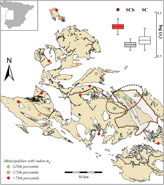
Figure 5. Regional map showing lithostratigraphic unit SC (Schist–Greywacke Complex slates and greywacke). According to the rank of their radon geometric means, sampled municipalities are displayed as follows: green crosses (<25th percentile); orange squares (25th–75th percentile); or red circles (>75th percentile). A star marks a municipality considered anomalous due to its high radon values. The ellipse with the dotted line highlights the patch of low radon values. The shaded area marks the extension of the local mountain range. The box plot represents the individual radon concentration values measured at the following types of municipality: municipality with anomalous radon data, municipalities over slates and greywacke within the shaded area (unit SCb), and the rest of the municipalities in unit SC.
Download figure:
Standard image High-resolution imageWe obtained the experimental variograms for units AP and Q (figure 6). Both of them correspond to a pure nugget effect, as can be seen from the theoretical model fit. This model entails a complete lack of auto-correlation at distances larger than the lag bin size.
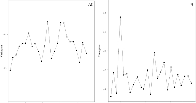
Figure 6. Experimental variograms for lithostratigraphic units AP and Q. The solid line represents the fitted pure nugget effect model.
Download figure:
Standard image High-resolution imageThe same results were confirmed by means of Moran's I (Cliff and Ord 1973). Moran's I ranges between −1 (perfect negative auto-correlation at global level) and 1 (perfect positive global auto-correlation), with values close to 0 indicating a random distribution. We used an inverse-distance weight matrix to compute the statistic, and a Monte Carlo permutation test (i = 1000) to assess its statistical significance. For plutonic rocks, we obtained Iobs = 0.066 (p = 0.051), whereas for Quaternary materials Iobs = 0.039 (p = 0.142). Both Iobs and p values indicate a lack of global auto-correlation.
The lack of a global spatial pattern (gradients or large-scale patches) suggests that precipitation and temperature regimes, which exhibit marked gradients N–S/SE through these two extensive LS units, do not exert a noticeable influence on radon indoors. Furthermore, given that the two units exhibit opposite behaviour regarding radon transport (impermeable matrix with highly permeable fracture zones versus highly permeable homogeneous material), it is reasonable to assume that this result may be extrapolated to all LS units excepting unit SC, which needs further analysis.
There are two issues regarding radon data from unit SC. First, one of the sampled municipalities displays a clearly anomalous behaviour (see box plot in figure 5) and was thus excluded from the study. The very high radon values (up to 15 000 Bq m−3) measured in this municipality can be attributed to the existence of an underlying uranium deposit (Arribas et al 1983).
Although this is a unique situation, other municipalities have close uranium deposits that could potentially increase indoor radon levels. The diffusion length of this gas in soil is only about 1.2 m, but advective transport by carrier gas also occurs at long distances (several hundred metres) (Etiope and Martinelli 2002). In addition, surface soils in the proximity of uranium deposits show enhanced 226Ra concentrations (up to two orders of magnitude higher than background levels), although this is a very local effect (Baeza et al 1994). For unit SC, we compared indoor radon data {xi} from five municipalities near uranium deposits (0.3–2 km) with those from the rest of the locations. The F test indicates equal variances for both groups (F = 0.5821; p = 0.094), whereas the two sample t-test proves equal means (t = 0.5346; p = 0.5929). Similar results are actually obtained when the analysis is replicated for unit AP, which also hosts several uranium deposits: F = 0.5841 (p = 0.062); t = 0.6405 (p = 0.522). Based on these results, we concluded that uranium deposits in granite and schistose rock do not have an influence on indoor radon levels at nearby population centres, at least when located at distances larger than 0.3 km (from the built-up area to the boundary of the ore deposit).
The second issue regarding radon levels in unit SC is the presence of a visually apparent large patch of minima that can be observed in figure 5. Most of the municipalities forming this patch are located in an isolated mountain range that forms a series of alternating ridgelines and valleys. They were considered as a distinct LS unit (SCb) solely in order to detrend the data and prevent bias in statistical inference.
We then grouped the individual  radon measurements made in dwellings at the km municipalities in each LS unit, m. For each of these data samples, {xi}m, we performed a normality test on the log-transformed values. If the sample size was larger than 50, we used the Kolmogorov–Smirnov test. Otherwise, we applied the Shapiro–Wilk test. All data sets follow lognormal distributions and, thereby, the statistical hypothesis test described in section 3.1 was performed. Table 2 shows
  for the different LS units, as well as other relevant statistical parameters.
The resulting map of currently identified radon-prone areas is shown in figure 7. All units classified as radon prone have average γ-dose rates greater than 100 nGy h−1, whereas some units with average values as high as 120 nGy h−1 are not radon prone. Also, at the geological unit level, γ-dose rate plays a role in determining radon risk but is not a good indicator above a certain threshold.

Figure 7. Map of radon-prone areas (shaded in pink), i.e. areas with  , for mainland Spain. Areas pending classification due to insufficient sample size are coloured in grey. The grey division lines mark the major water catchment areas.
Download figure:
Standard image High-resolution image
5. Future developments
Grey areas on the map (figure 7) indicate those LSs that exhibit Rγ > 66 nGy h−1 and lack enough measurements (n < 27) to allow calculation of the 90th percentile of radon in dwellings. With an envisaged running time of three years, the following developments are underway with the aim of completing the map shown in figure 7 and verifying its consistency with the intended application.
- Carry out a sampling campaign started in 2013 to retrieve the necessary data from all LS units in order to cover the whole territory of Spain (including the Balearic and the Canary Islands).
- Expand the study on radon spatial variability within LS units using precisely geo-reference measurements.
- Evaluate the performance of the approach presented in this paper in relation to methods based on a high density of measurements in two Spanish regions of different climates and geologies.
On the basis of such a map, CSN will launch regulation addressing the problem of populations geographically associated with high radon levels in Spain. In the long term, the radon-prone area delineation will be subject to periodic review by CSN as the radon measurement database grows, driven forward by national and local radon protection policies.
6. Conclusions
The method presented in this paper to delineate radon-prone areas is, from a cost-effectiveness point of view, an advantageous approach in developing a national radon policy. Because it makes use of frequently available environmental information (such as geological or γ-radiation maps), it requires a relatively small number of indoor radon measurements. This allows a more prompt implementation of protection strategies, preferentially targeted to the areas most at risk, thus optimising resources and reducing regulatory burdens.
It also shows limitations in the sense of spatial accuracy and that maps developed on actual in-house measurements would always provide the most reliable estimate. More elaborate predictive models accounting for effects such as local soil permeability or dwelling characteristics could also perform better. As conceived here, the radon-prone area map is the first version of a long-term dynamic project to be corroborated and improved as new precisely geo-referenced radon data become available from specific sampling campaigns and from radon testing required by regulation. The continuous input of radon measurements is essential to improve the accuracy of the defined areas and, consequently, to ensure better protection for individuals.
External γ-dose rate has been proved to discriminate non-radon-prone municipalities excellently. Above the cut-off of 66 nGy h−1, predictions on the probability of exceeding the reference level must be made not at the municipality level but at the lithostratigraphic unit level. We have proposed a hypothesis test on the 90th percentile for the radon indoors distribution that controls the probability of both false positive and false negative results. This implies acknowledging the uncertainty on making the right decision on area classification rather than relying on a point estimate.
Footnotes
- 3
For n = 6 the error associated with the geometric mean estimate is around 50% (Hewett 1995).
- 4
To a certain extent, permeability is determined by LS unit. However, where the predominant flow mechanism is through fractures (e.g. igneous or metamorphic rocks), local permeability can be very variable, up to several orders of magnitude, whereas more permeable lithologies, dominated by inter-granular flow, present a rather homogeneous local permeability.