

Abstract
The destruction of Kolmogorov–Arnold–Moser surfaces in a Hamiltonian system is an important topic in nonlinear dynamics, and in particular in the theory of particle orbits in toroidal magnetic confinement systems. Analytic models for transport due to mode-particle resonances are not sufficiently correct to give the effect of these resonances on transport. In this paper we compare three different methods for the detection of the loss of stability of orbits in the dynamics of charged particles in a toroidal magnetic confinement device in the presence of time dependent magnetic perturbations.
Export citation and abstract BibTeX RIS
I. Introduction
Only through resonance can orbits be significantly modified in an integrable conservative dynamical system. Without resonance the trajectories in phase space occupy Kolmogorov–Arnold–Moser [1] (KAM) surfaces that prohibit diffusion without particle collisons, and in the presence of collisions only relatively slow neoclassical diffusion results. Isolated resonances modify particle distributions by phase mixing in islands and overlapping resonances allow stochastic transport. Often individual perturbations of an integrable system are so small that the system is very far from Chirikov overlap, and thus the destruction of the last KAM surface is not a good paradigm for the examination of diffusive transport. Even if nearby resonances overlap the random phase approximation is not well suited to describe the transport in many cases. It can be necessary to understand the domains of broken KAM surfaces for each perturbation separarately, and to find the resulting transport due to the action of all modes together. In this work we compare three methods of determining the stability of orbits in a Hamiltonian system, the method of frequency analysis [2–4], that of the fast Lyapunov indicator [5] (FLI) and that of phase vector rotation [6, 7].
Although the methods apply to any conservative Hamiltonian system, we consider here the dynamics of charged particles in an axisymetric toroidal magnetic confinement system, perturbed by time dependent magnetohydrodynamic (MHD) modes of a given spectrum. As well as providing an interesting Hamiltonian system of two variables, it is of important practical interest in the pursuit of controlled thermonuclear fusion. In the absense of perturbations the system is integrable, the orbits forming a phase space of invariant tori with two degrees of freedom, corresponding to poloidal and toroidal motion in a topological torus. Typically in experiments several small amplitude modes are present, each with a different frequency and toroidal and poloidal mode numbers [8]. The modes are driven unstable by the free energy of a high energy particle distribution such as fusion produced alpha particles and thus are expected in any magnetic fusion experiment. Although Poincaré sections can be made for each mode individually, such plots are often well below Chirikov threshold [9], individual modes not producing diffusion because of the Nekhoroshev theorem [10] and only the synergistic action of the collection of modes leads to particle transport [6, 7].
Using the guiding center drift approximation a particle orbit in an axisymmetric toroidal system is completely described by the values of the toroidal canonical momentum  , the energy E and the magnetic moment μ. Particle spatial coordinates are given by
  , respectively the poloidal flux coordinate, a label of the unperturbed topologically toroidal flux surfaces, and the poloidal and toroidal angles. The magnetic field is given by

where  ,
,  and
and  are functions determining the form of the equilibrium. The toroidal field strength is given by g, the poloidal field by I, and δ is related to the nonorthogonality of the coordinate system. The guiding center Hamiltonian is
where  is the normalized parallel velocity,
  is the particle velocity parallel to the magnetic field, μ is the magnetic moment, and
  the electric potential. The field magnitude B and the potential may be functions of
  , θ and also ζ if axisymmetry is broken. We consider perturbations with the frequency well below the cyclotron frequency and ignore particle collisions, so μ is conserved and may be considered a constant parameter. The construction of equilibrium fields involves the solution of the Grad-Shafranov equation and is well known. The equilibrium used for most of this paper is a simple circular large aspect ratio equilibrium with the field line helicity
  quadratic in the minor radius and with q on axis of 0.8 and q = 4 at the plasma edge. The major radius is 100 cm, the minor radius 25 cm and the magnetic field on axis is 20 kG. The details of the equilibrium and the high energy particle distribution determine the mode spectrum. In the following we will use a simple ad hoc mode spectrum, sufficient to display the properties of each method.
Canonical momenta are

where ψ is the toroidal flux, with  , the field line helicity. The equations of motion in Hamiltonian form are
Hamiltonian equations for advancing particle positions in time, also in the presence of time dependent flute-like perturbations of the form  with
with  the equilibrium field and
  can easily be derived [11]. Since the equilibrium is axisymmetric, the toroidal mode number n is well defined, so the mode frequency
  depends only on n. Each mode normally possesses several poloidal harmonics given by m. The eigenfunctions of the perturbation
  have the dimensions of length, and are zero at the axis and the plasma edge. We will cite amplitudes giving the maximum value in terms of the major radius R. The guiding center equations including MHD perturbations are realized using a fourth order Runge–Kutta algorithm in the code ORBIT [12]. The units are conveniently defined by the on-axis cyclotron frequency
  (time) and the major radius R (distance). Another characteristic time is the toroidal transit time for a particle of a particular energy and
  at the magnetic axis.
The variables E and  are constant in an unperturbed system, but
  and
and  are not action variables so
  and
and  are not constant in time. However, in an axisymmetric system, without perturbations, the system is integrable, and orbits close in the poloidal plane in a time
  , which depends on the values of E and
  and thus because of the toroidal precession, frequencies of the system are given by
  , and
, and  , with
  the toroidal motion of the orbit in time
  . One can also use the the helicity of a particle orbit in the mode frame,
  , where
  and
and  are the toroidal and poloidal angles traversed in time t, and the time is taken to be large compared to
  , useful because it must be equal to a low order rational for a resonance to occur. An orbit closing upon itself after a finite number of poloidal and toroidal transits is a necessary but not sufficient condition for resonance to occur. In figure 1 is shown a mapping of points in the
  , E plane describing confined orbits into the plane of
  ,
,  , demonstrating the topological equivalance of these variables to action angle variables within this range. The energy is in units of keV. The frequencies are normalized to the toroidal transit frequency of an on-axis particle with energy 12 KeV and
  . In the equilibrium used they have a value of 10 kHz. The introduction of symmetry breaking perturbations destroys the one to one character of the map from the
  , E plane into the plane of
  ,
,  , normally producing folds along singular surfaces.

Figure 1. Mapping of the  , E plane into the frequency plane, showing that the variables
  , E are topologically equivalent to action angle variables.
Download figure:
Standard image High-resolution imageIn section II we discuss kinetic Poincaré plots as a means of examining the destruction of KAM surfaces and give two cases to be examined with the three methods. Section III considers the method of frequency analysis, section IV, the fast Lyapunov indicator, first introduced in the analysis of the stability of the solar system, and section V that of phase vector rotation. Conclusions are given in section VI.
II. Kinetic Poincaré plot
We are interested in the case of the interaction of particles of arbitrary pitch with low amplitude modes of nonzero frequency. It is fairly easy to assess the effect of a particular mode of a single n, ω, but possibly with many poloidal harmonics m, on a particle distribution by examining a Poincaré plot for a particular choice of either co-moving and trapped or of counter-moving particles, which we refer to as a kinetic Poincaré plot to distinguish it from a plot of the magnetic field. Points are plotted in the poloidal cross section whenever  with k integer.
The toroidal motion then gives successive Poincaré points in the poloidal cross section  , θ, or better, since
  and E are constant in the absence of perturbations, the
  plane or the
  plane.
  , E, and
  are simply related for a mode of a single frequency and toroidal mode number. Individual modes produce islands in the phase space of the particle orbits, which through phase mixing produce local flattening of the particle distribution. In addition, overlap of these islands, the Chirikov criterion, leads to stochastic transport of particles [9, 13]. Such a plot shows the canonical division of orbits into those following good KAM surfaces, isolated islands bounded by separatrices, and stochastic domains.
To obtain a kinetic Poincaré plot the orbits must be initiated with a fixed value of μ and  . Here
  is simply the particle energy in the frame of the rotating mode and is conserved in the presence of this mode, an orbit moving in the
  , E plane only along a line with this slope. A plot of orbits with fixed μ and energy E does not give a coherent plot; it contains intersecting surfaces, since it is really an overlaying of plots with different values of c. Thus a plot can be obtained only for a perturbation consisting of modes with a single value of
  , typically meaning only a single frequency and n value, although it may contain many poloidal harmonics m.
Orbits in a general toroidal equilibrium are classified according to whether they are poloidally trapped or passing, whether they circle the magnetic axis, and the direction in which they circle toroidally, dividing the space of  into distinct domains [11]. In the following we will restrict ourselves for simplicity to a single domain, that of co-moving passing orbits. We take a simple example, consisting of a perturbation with a single harmonic, with m = 6, n = 5, a frequency of 10 kHz, and a simple global radial structure for α. We will examine first KAM stability along a single line in the
  volume, with
  keV,
keV,  and the energy chosen to be 12 keV at the plasma edge,
  . This simple example will serve as a test case for the three methods of determining the breaking of KAM surfaces in the space of particle orbits.
The resulting Poincaré maps are shown in figure 2, spanning almost the full domain of confined orbits along this line in the  , E, μ volume, determined by the value of
  . Principal island chains are seen at the resonances given by
  with, starting from the right,
  and 11/5. The range of q covered does not include q = 1, otherwise there would also be visible a
  island on the far right. In between these island chains there are also higher order Fibonacci sequence chains, obtained from modes m/n and
  through
  not always visible without using higher resolution Poincaré plots. Clearly seen is only the 19/10 resonance between 10/5 and 9/5. The quantity
  is used to distinguish the number of islands in the chain from the poloidal mode number m of the perturbation, m = 6.

Figure 2. Kinetic Poincaré plot showing all confined orbits with  , with energy at the plasma edge of 12 keV, and
  keV, and with a perturbation of a single harmonic with m/n = 6/5, frequency of 10 kHz,
  .
.
Download figure:
Standard image High-resolution imageThis plot illustrates the difficulty in analytically predicting resonance location and strength in this system. Conventional wisdom has it that a perturbation with poloidal and toroidal mode numbers m/n will produce resonances due to the m = 1 character of the orbital shift due to drift motion with islands at  . We see that the actual situation is much more complex, with
  ranging from 6 to 11 even with the perturbation far from Chirikov overlap, and with these resonance islands all practically of the same order in size. Resonance locations can be found by numerical integral methods, [14–16], but while these methods give the location, they do not provide the resonance width and thus the extent of the effect of the mode on transport.
The second case, shown in figure 3 has the same perturbation but a larger amplitude, by a factor of 8, producing some chaotic domains with remnant islands imbedded in them. The perturbations used are smooth and global radially, not localized, so they overlap everywhere. Although some good KAM surfaces still exist, transport in such a system is very complicated. In addition, as has been well demonstrated in simple systems [17], transport even well above the breaking of the last KAM surface involves many long time correlations, and is not well described by a random phase approximation. The transport is characterized by Levy flights, and can be of the form  with
with  subdiffusive or
  superdiffusive [18]. However in the present case the domains of broken KAM surfaces are too small to allow significant long time averages. Probably the only useful measure is the time necessary for the flattening of a distribution in the domain, given by the island rotation frequency.
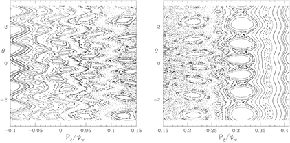
Figure 3. Kinetic Poincaré plot showing all confined orbits with  , energy at the plasma edge of 12 keV, and
  keV,
keV,  .
.
Download figure:
Standard image High-resolution imageThese examples are sufficient for the examination of methods for the determination of broken KAM surfaces, containing resonant islands of various size, regions of unperturbed surfaces, regions with highly perturbed surfaces with no islands, and stochastic domains. A Poincaré plot is useful for a single line in the  , E, μ volume, but not useful to characterize points in the volume according to whether they belong to good KAM surfaces or are broken, as it depends on visual inspection and gives information along one line at a time.
Both the method of frequency analysis and FLI given in the references had the luxury of knowing the phases of the O-points in the Poincaré plots of the system, and therefore being able to choose initial conditions for orbits so that they intersected the O-points at the resonant values of the action variable. This provides for a very clear demarcation of a resonance and of the Arnold web because it is impossible to miss the center of the resonance. This is not the case in general, where one cannot know these phases, as is clear from the plot of the resonances in figures 2 and 3. Higher order Fibonacci resonances will not in general appear at the same phases as the principal ones. We compensate for this lack of knowledge where possible by initiating orbits with different phase values, to maximize the probability of intersecting the resonance.
III. Frequency analysis
The works of Laskar [2–4] discuss various averaging means of obtaining frequencies associated with orbits. Since we are interested in resonances, the orbit helicity h is a quantity which is heuristically useful. Orbits are initiated along a single line in the  volume, with
  keV,
keV,  and the energy chosen to be 12 keV at the plasma edge,
  , ie the same set of orbits used for the kinetic Poincaré plots shown above. If an orbit is followed for a sufficient length of time the bounce motion of a particle trapped in an island is negligible, and the observed helicity of the orbit is simply the helicity of the resonance. The interior of an island thus produces a range of parameter values in which h is constant. At the edges of this domain there is a jump in the value of h and hence an easily observed singularity in the second derivative. In our case μ is fixed and the initial value of
  characterizes the orbit. We typically used a total of one thousand orbits, spanning the range of confined orbits in the system used in figure 2, and a time of one thousand transits.
The results of this method depend on the phase between the orbit trajectory and the mode phase. In figure 4 is shown how the results vary for a single resonance, with plots made with different phases between orbit and mode. If the trajectory intersects the mode at an elliptic point the range of constant h is as broad as the island width, but if it intersects the island at a hyperbolic point it has zero width. For a given phase the plot of helicity is approximately symmetric about the rational surface. The phase dependent island width shown by this method complicates the analysis if the mode phases are not known or if they vary from resonance to resonance, giving widths of regions with constant h that do not represent the maximum island width for all resonances.
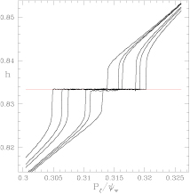
Figure 4. Frequency analysis, with different phases between the node and the particle trajectory. The width of the parameter range in which h is constant gives the width of the island at the point of intersection of the orbit with the mode.
Download figure:
Standard image High-resolution imageIII.A. Case I
In figures 5 and 6 are shown the results for the same orbits shown in figure 2. Following Laskar, we varied the number of orbits used, and hence the spacing in  as well as the the time step in the integration process to obtain good results. Flat domains of h are seen for the major island chains, and the numerical second derivative of the helicity [
 ] clearly indicate the edges of major island chains as well as three of the first order Fibonacci chains. The red lines in figure 5 are at helicities of
  , in excellent agreement with the flat domains of the function h. In the domains of good unperturbed KAM surfaces
  is seen to be very smooth. The only drawback of this method is that the flat regions of h do not give the full island width unless the orbit happens to intersect the island at an elliptic point. We have managed to choose a phase so that the islands are well indicated, so the widths are apparent. Note that the same phase must be used for all orbits, using random values of phase for each point would make h practically a random function of
  .
.
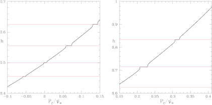
Figure 5. Frequency plot for poloidal rotation in the presence of the perturbation. Shown is the helicity h versus  with the perturbation shown in figure 2, with
  . The red lines are at helicities of
  , in excellent agreement with the flat domains of the function h.
Download figure:
Standard image High-resolution image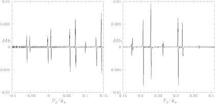
Figure 6. Frequency plot for poloidal rotation in the presence of the perturbation. Shown is the numerical second derivative  with the perturbation shown in figure 2, with
  .
.
Download figure:
Standard image High-resolution imageIII.B. Case II
In figures 7 and 8 are shown the results for the same orbits shown in figure 3, with  . In this plot h is flat at most of the remaining imbedded islands and also at higher order Fibonacci islands in between them. Island 8/5 is missing although present in the Poincaré plot, only an extended chaotic domain is seen. The numerical second derivative of the helicity [
 ] shows the remaining large islands as well as Fibonacci islands in between each of the principal resonances, with large resonances at 10/13 and 10/19. There are three clear domains of chaos visible, near
  , from 0.1 to 0.2, and from 0.24 to 0.27, surrounding the remaining isolated islands.
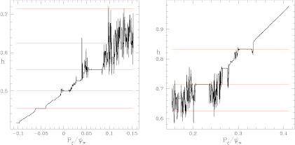
Figure 7. Frequency plot for helicity h in the presence of the perturbation. Shown is the helicity h versus  with the perturbation shown in figure 3.
  .
.
Download figure:
Standard image High-resolution image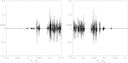
Figure 8. Frequency plot for helicity h in the presence of the perturbation. Shown is the numerical second derivative  with the perturbation shown in figure 3.
  .
.
Download figure:
Standard image High-resolution imageIV. Fast Lyapunov indicator
The fast Lyapunov indicator (FLI) is another means to determine the destabilization of orbits [5]. Consider two very nearby orbits and examine the distance d between them in the  plane. The normal Lyapunov is the limit of ln(d)/t for large time t. The FLI is the value
  at fixed time t, which keeps track of the topological differences between resonant regular motion and KAM tori. Using the usual Lyapunov number, for
  both domains give zero, but at finite time the linear dependence of d on time for points at good KAM surfaces distinguishes these points from island interiors, where d remains relatively constant. To account for the fact that the phase location of the islands is unknown, several different orbit pairs were used for each value of
  with different phase with respect to the mode and the minimum value λ taken for each
  . Thus the value of λ is given with the inital conditions of the orbit closest in phase to being at an island elliptic point. The time t was chosen to optimize the resolution of the calculation. The pair separation was chosen to be
  , limiting the detection of islands to those larger than this.
IV.A. Case I
Shown in figure 9 is the fast Lyapunov indicator for the perturbation shown in figure 2. Five orbit pairs were initiated at each value of  , and the minimum value of the separation betwen the points taken for λ. We find the distance between the points d to be a more sensative indicator than the logarithm of d. The islands are seen as regions where the indicator is near zero. Domains with good KAM surfaces show linear separation of the orbit pairs in time and thus nonzero λ. This method roughly indicates the width of the islands, but not exactly because there is also some spread of orbit pairs located inside an island due to relative rotation rates about the island elliptic point.

Figure 9. The fast Lyapunov indicator for case I.
Download figure:
Standard image High-resolution imageIV.B. Case II
Shown in figure 10 is the fast Lyapunov indicator for the perturbation shown in figure 3. This indicator gives only a very qualitative indication of the stochastic domains and remnant islands. One can roughly make out regions where the remnant islands exist, but with very limited accuracy.
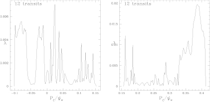
Figure 10. The fast Lyapunov indicator for case II.
Download figure:
Standard image High-resolution imageV. Phase vector rotation
Another method for numerically determining the existence of or the destruction of good KAM surfaces can be obtained using the method of phase vector rotation [6, 7]. Consider following two orbits located nearby one another. Examine a Poincaré section in  and define the angle χ to give the orientation of the vector joining them in this plane. If good KAM surfaces exist χ can change by at most an angle of π, due to their relative velocity in the angular coordinate.
However two orbits within an island rotate around one another with χ increasing with the rotation about the island, also referred to as the bounce frequency of a particle trapped in the wave, which increases with the size of the island. The rate of change of χ is a function of distance from the island O-point, dropping to zero at the separatrix. Pairs of orbits are illustrated in figure 11, showing vectors between the nearby points in the  plane on good KAM surfaces and in a resonance.
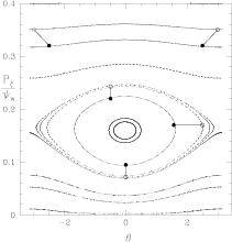
Figure 11. The  plane showing a single m = 1 resonance island, and vectors between nearby points on good KAM surfaces and in the island. On nearby KAM surfaces the phase vector can rotate by at most π, whereas a phase vector in an island rotates through
  with a period given by the trapping bounce time. (Reprinted from [6]. © 2012 Elsevier).
Download figure:
Standard image High-resolution imageThus we determine the nonexistence of good KAM surfaces by examining nearby pairs of orbits, looking for phase vector rotation χ exceeding π. Because local perturbation of orbits can cause χ to excede π by some small amount, whereas χ continues to rotate in an unbounded manner in an island, we record the time at which  , thus giving the rotation frequency
  as a function of the initial position of the orbit. The pair separation was chosen to be
  , limiting the detection of islands to those larger than this, and the time used was 500 toroidal transit times, making the minimum observable frequency to be
  , normalized to the toroidal transit frequency. The results depend on the phase relation of the orbit with respect to the mode, but using this method one can simply launch a few pairs of orbits at a given value of
  with different phases and select the maximum value of
  , corresponding to the pair which is closest in phase to the island elliptic point.
V.A. Case I
Results are shown in figure 12 for a perturbation amplitude of  . This method clearly indicates the presence of phase space islands. In addition to the major resonances seen in figure 2 the first order Fibonacci resonances, 13/10, 15/10, 17/10, and 19/10 are all visible. The magnitude of the phase vector rotation
  gives the time scale for phase mixing of orbits trapped inside the island. Note that for larger islands one even obtains the internal profile of the rotation frequency. To achieve this several orbit pairs are necessary, with different phases with respect to the mode, as was used for the FLI. Note that the phase vector rotation and the FLI are obtained with the same calculation. 2000 orbits, 500 transits.
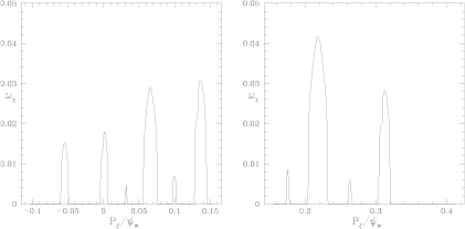
Figure 12. Vector rotation plot showing rotation frequency versus  . The frequency is in units of the on-axis transit frequency, largest islands exhibiting the fastest phase mixing. Mode amplitude is
  .
.
Download figure:
Standard image High-resolution imageV.B. Case II
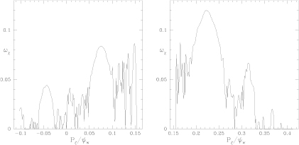
Results are shown in figure 13 for the larger perturbation. The major remnant islands are seen, and it is also possible to see overlap of these chains by noting that there is no region in which  in between some chains, indicating that the island is surrounded by a stochastic sea, with no intervening KAM surfaces. Note that the frequencies for phase mixing are three times as rapid as in the lower amplitude case shown in figure 12, scaling as the square root of the perturbation amplitude. It is interesting that the stochastic domains do not produce more rapid phase vector rotation than the coherent rotation present in the remnant island centers. Taking the maximum values of
  over the mode-orbit phase relations always clearly shows the centers. The edge of the remnant islands can even be inferred by the minimum values of
  surounding it, where overlap with another island chain and chaos intervenes. Again for these calculations 1000 orbits were followed for 500 transits.
Figure 13. Vector rotation plot showing rotation frequency versus  for a perturbation amplitude of
  . The frequency
  is in units of the on-axis transit frequency, largest islands exhibiting the fastest phase mixing.
Download figure:
Standard image High-resolution image
The Arnold web consists of resonances in the plane of the action variables. It is an open set, dense but with small measure if the perturbations are small. In many cases the resonant lines form complicated web like patterns in this plane. Arnold diffusion is diffusive motion along a resonance line this plane.
Examples of Arnold web construction for the methods of frequency determination and FLI are given in the cited references, so we will not reproduce these methods here. The analysis of the single line in the  plane given in the preceding sections is sufficient to judge the capabilities and shortcomings of the methods without examining the whole plane of the Arnold web. In the system under study the Arnold web is simpler than in many Hamiltonian systems, consisting almost entirely of nonintersecting lines of resonances, occasionally broken in intervals. However there are often several perturbations present of different frequencies, which thus cannot be observed in a single Poincaré plot, and the action of these modes together produces significant chaotic transport. In the present work the resonances are always observed to be nearly vertical in the plane of
  , E, almost parallel to the bounding surfaces, given on the left by contact with the plasma boundary, and on the right by the magnetic axis. No resonance lines with nearly constant energy E are observed. Thus in the particular system of particle orbits in a toroidal confinement device, the Arnold web does not lead to the possibility of significant transport. It could provide some movement in the energy variable, but nothing leading to paticle loss or profile flattening.
VI. Conclusion
Resonance is the only means by which modes can modify particle distributions, through Landau mixing and stochastic motion due to the overlap of resonances. Thus the determination of the location and extent of resonances due to perturbations is important for understanding induced transport. Three methods of determining the destruction of KAM surfaces were compared, that of frequency analysis, that of the fast Lyapunov incicator, and that of phase vector rotation. The method of phase vector rotation appears to be a more efficient and reliable means of finding resonances. It contains more information, giving the extent of island structures, even when immersed in a stochastic sea, and also gives a measure of the mixing time within the islands. The mixing time, given in figures 12 and 13 by  , directly gives the time scale for profile flattening within the domain of broken KAM surfaces, and thus provides transport information even when other quantitative measures such as diffusion rates are lacking.
Acknowledgment
The author acknowledges useful discussions with J Laskar. This work was partially supported by the U.S. Department of Energy Grant DE-AC02-09CH11466.