Abstract
On 14 July 2011, the two ARTEMIS spacecraft observed a chain of flux ropes generated by reconnection in the Earth's magnetotail. The flux ropes are found to extend more than 90 ion inertial lengths out of the reconnection plane. We analyze six of these flux ropes by employing a novel combination of two-spacecraft-timing for their global orientation and Grad–Shafranov reconstruction (GSR) for their local orientation. We find that their diameter was ∼10 ion inertial lengths, temporal separations ∼100 ion gyroperiods, and that their speed increased from ∼30% to ∼70% of the Alfvén velocity. Given their temporal and spatial separations, we can infer that they were produced sequentially via a secondary instability. All of the flux ropes were tilted in the current sheet plane, suggesting that the secondary instability grew along the X-line in the direction of the electron current (−YGSM). The first five had a tilt between −14° and −26°. Based on the GSR axes their shape became increasingly complex over a period of ∼300 gyroperiods indicating kinking. The sixth event was again rather linear, and had a larger tilt (−38°), cross-section and core magnetic field; these changes are most likely related to a change in the boundary conditions.
Export citation and abstract BibTeX RIS

Content from this work may be used under the terms of the Creative Commons Attribution 3.0 licence. Any further distribution of this work must maintain attribution to the author(s) and the title of the work, journal citation and DOI.
1. Introduction
Magnetic reconnection across the Earth's magnetotail current sheet enables the rapid release of energy stored in the magnetotail lobes, and is therefore ultimately responsible for powering geomagnetic substorms and storms (e.g., [1]). Extremely precise in situ measurements by satellites have stimulated considerable progress in recent years in our understanding of collisionless reconnection (e.g., [2, 3]).
A common feature of (magnetotail) reconnection are discrete structures such as magnetic islands (e.g., [4]). The sketch in figure 1 shows a cut in the reconnection plane, with an island entrained in tailward flow from the X-line. The main observational signature of an island is a bipolar variation in the north-south component of the magnetic field (BZ). A tailward traveling island will have a field component pointing in the +Z direction in its leading part, and in the −Z direction in its trailing part [5, 6], and a spacecraft located in the plasma sheet (red dashed arrow) will observe this variation accompanied by the reconnection jet. In contrast, a spacecraft located outside the plasma sheet in the lobe (dark blue dashed arrow) will observe the magnetic field signature of a traveling compression region (TCR): the lobe field lines draped around the bulge that constitutes the island [7]. This also results in a ±BZ variation, together with an increase in the field strength [8], but no plasma jet observation. Although the magnetic fields in the magnetotail are, to first order, anti-parallel, even a small guide field (i.e., the magnetic shear across the current sheet <180°) will ensure that these structures are open and are best described as flux ropes. Accordingly, it is important to understand their three-dimensional (3D) form and connectivity [4].

Figure 1. Cartoon illustrating the geometry of a typical flux rope encounter which results in a positive/negative bipolar signature in the BZ time series. The Earth is to the right, the plasma sheet is shaded orange and a possible core field (BY; into the page) is displayed. The light blue arrows indicate the plasma flow and the dashed arrows possible spacecraft trajectories.
Download figure:
Standard image High-resolution imageOn the largest scales, plasmoids are produced in association with a substorm, when reconnection at the near-Earth neutral line detaches a region of the plasma sheet [9, 10]. Magnetic islands generated by multiple X-lines have been observed on the meso-scale [6]. On smaller scales, secondary islands created at a single pre-existing X-line have been reported [11–13]. The production of secondary islands is of significant interest because they may act to modulate the reconnection rate [14], and may also act as sites for particle acceleration [15, 16].
The 3D structure of flux ropes is also closely related to the 3D structure of reconnection itself. Historically, simulations capable of resolving collisionless reconnection physics have mainly been performed in 2.5 dimensions owing to the availability of computational resources (e.g., review by [17]). Regarding fully 3D simulations, in the context of the Earth's magnetotail, two-fluid simulations show that reconnection will begin at a point on the current sheet, and then develop into an X-line by spreading in the out-of-plane direction (Y direction in figure 1) [18]. Simulations show that for anti-parallel reconnection, the X-line is expected to grow in the direction of the current carrier [18–22]. In a Harris sheet, ions are the main current carriers (e.g., [18]). Observationally, some studies have identified electrons as the main current carriers in the magnetotail plasma sheet [23], particularly in the thin current sheets that occur prior to reconnection onset in the near-Earth region [24], while others suggest ions in the duskside [25]. Regarding the formation of flux ropes, recent 3D particle-in-cell (PIC) simulations of a reconnecting planar current sheet show the generation of multiple tilted flux ropes, sometimes on a hierarchy of scales [26, 27].
Attempts to observationally determine the 3D structure of reconnection in the Earth's magnetotail, and in particular variation along the X-line ultimately require multi-point satellite measurements. For example, although initial statistical analysis led to a suggested plasmoid width of ∼40 RE [28], essentially filling the whole magnetotail, recent direct measurement shows that the plasmoid width can be spatially limited to a few RE [29]. A statistical analysis of Geotail data showed that flux ropes are often tilted in the plane of the current sheet [5], but that there can be considerable variation in the angle of tilt. Tilting of flux ropes over relatively small scales (a few RE in Y) has been directly confirmed by multi-point observations for both Earthward [30] and tailward [31] propagating structures. It has been proposed that such tilting may arise due to spreading of the X-line, or due to 'tethering' of the flux rope to the ionosphere at one end or the other, at least for tailward propagating structures [31].
As such, the 3D structure of flux ropes in the Earth's magnetotail still remains relatively unknown, partly due to a lack of widely separated satellite measurements in the out-of-plane direction. To address this, here we present a detailed case study of a chain of reconnection-generated flux ropes observed by the two ARTEMIS satellites (P1 and P2) [32, 33] on 14 July 2011. Concentrating on six events, we examine their timing and orientation, and use Grad–Shafranov techniques to determine their structure.
2. Datasets and methods
2.1. ARTEMIS data
We have analyzed dc magnetic field data from the Flux Gate Magnetometers (FGM; [34]), plasma data from the Electrostatic Analyzers (ESA; [35]) and high energy ion data from the Solid State Telescopes (SST; [36]). We use the geocentric solar magnetospheric (GSM) coordinate system where the XGSM direction points from the Earth to the Sun, the XZGSM plane contains the magnetic dipole and (X–Y–Z)GSM is right handed. As such, the magnetotail current sheet lies parallel to the XYGSM plane, and reconnection typically results in jets in the ±XGSM direction with the X-line along the YGSM direction. During the early mission phase P1 and P2 were often separated by large distances (∼10 RE) in YGSM, which is suitable for studying the 3D properties of magnetic reconnection.
2.2. Modeling
2.2.1. Two-spacecraft-timing.
We employ a two-spacecraft-timing analysis to obtain the global orientation of the flux ropes in the XYGSM (nominal plasma sheet) plane. In other words, we assume that the flux rope is a straight line propagating at a constant speed. Starting from spin resolution (∼3 s cadence) measurements, we re-sample the data to a common, equidistant time grid of 1 s resolution using linear interpolation. For each rope, the midpoint between the extrema of the variation in ±BZ is taken as the reference time. We assume that the speed of the flux rope is the same as the observed jet velocity, i.e., Visl ∼ VX, taken at the reference time. Our results are not very sensitive to this assumption. The tilt angle θ2sc from the YGSM axis is then given by

where Δtsc = t1 − t2 is the time difference between the spacecraft, and ΔXsc and ΔYsc are the spatial separations of the spacecraft.
2.2.2. Grad–Shafranov reconstruction.
This technique recovers the local orientation of the flux rope axis based on the in situ measurements of an individual spacecraft, and a two-dimensional (2D) map of the magnetic field in a region around the spacecraft trajectory [37–39]. The reconstructed flux ropes are assumed to have translation symmetry with respect to an invariant axis direction. The 2.5-dimensional magnetic flux ropes with the invariant axis along z axis are described with the Grad–Shafranov equation:

where A is the magnetic vector potential, such that
 , and the magnetic field vector is B = [∂A/∂y, −∂A/∂x, BzA]. The plasma pressure, the pressure of the axial magnetic field and thus their sum
 (transverse pressure) are functions of A alone. We solve equation (2) numerically.
The crux of the technique is the determination of the flux rope invariant axis direction, which is based on the assumption of constant magnetic vector potential and transverse pressure on common magnetic field lines. Pt(A) consists of two branches corresponding to the parts of the spacecraft trajectory moving inward and outward of the flux rope. For the optimal direction of the invariant axis the two branches coincide. The errors of this method have been estimated so far only by comparison with benchmark MHD-simulated flux ropes. According to [40] the typical error for the invariant axis determination is 5°–10° and 5°–25° for low-impact and high-impact events, respectively.
The reconstruction procedure is carried in the de Hoffmann–Teller (dHT) frame, i.e., a co-moving frame of reference, in which the electric field E' ideally vanishes so that from Faraday's law,
 , the reconstructed magnetic structures are time-stationary. The quality of the dHT frame is assessed by the correlation coefficient cc between the components of −V × B and the corresponding components of −VdHT × B, where V and B are the plasma flow velocity and magnetic field measured in situ, respectively, and VdHT is the velocity of the dHT frame. When cc = 1 all electric fields in the frame are eliminated. The optimal de Hoffmann–Teller speed was estimated as the one that provides the highest value of cc.
3. Overview of the event
Figure 2 (top) shows the locations of P1 and P2 on 14 July 2011 at 10 : 00 UT in the XZGSM plane. P2 (red) was located at XGSM ∼ −53 RE, ZGSM ∼ 2 RE with P1 (blue) below it at ZGSM ∼ −3 RE, and slightly tailward (XGSM ∼ −59 RE). The bottom panel shows the projection in the XYGSM plane. The separation of P1 and P2 in the YGSM direction was more than 10 RE. P2 was close to midnight (YGSM ∼ 2 RE) while P1 was duskward from it (YGSM ∼ 14 RE). (Note that duskward refers to YGSM > 0 and dawnward refers to YGSM < 0.) During the interval under consideration, P1 and P2 moved ∼1 RE in the −YGSM direction whilst retaining their separation.

Figure 2. Locations of the two ARTEMIS spacecraft (P1 and P2) as well as Moon and Earth on 14 July 2011 at 10 : 00 UT. The top panel shows the projection in the XZGSM plane and the bottom panel the projection in the XYGSM plane, i.e., parallel to the plane of the magnetotail current sheet.
Download figure:
Standard image High-resolution imageFigure 3 shows observations from both satellites between 09 : 30–11 : 30 UT. The top four panels display data from P1: from top to bottom we show the ion energy spectrogram (energy flux as a function of energy and time), the magnetic field strength, the magnetic field components and the ion velocity. Data from P2 is shown in the same format in the bottom four panels. Initially, P1 was located in the southern lobe, outside of the plasma sheet, as indicated by the low density of ∼0.05 cm−3 and negative BX. At just before 11 : 10 UT P1 entered the plasma sheet. In contrast, P2 was located mainly in the plasma sheet, as indicated by the weaker magnetic field strength and the higher density of ∼0.1 cm−3. Examining the P2 observations in more detail, the satellite was also located below the tail current sheet (BX < 0) until ∼10 : 38 UT. This suggests that the tail current sheet was displaced to ZGSM > 0.
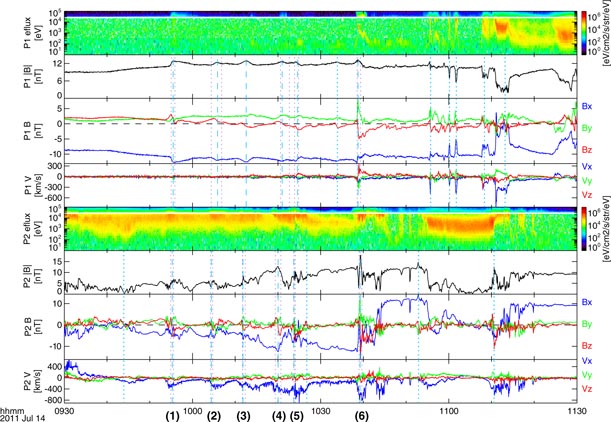
Figure 3. ARTEMIS P1 (top) and P2 (bottom) observations from 09 : 30 to 11 : 30 UT. The four panels show for each spacecraft the ion energy spectrogram, the magnetic field magnitude, the three magnetic field components, and the three ion velocity components. The vertical light blue lines indicate the flux rope and TCR signatures: the six events observed by both spacecraft are depicted with dashed lines and black numbers, while the ones seen by single spacecraft are depicted with dotted lines. The purple dotted lines depict the time boundaries of the unperturbed flux rope obtained from the Grad–Shafranov reconstruction (figure 4).
Download figure:
Standard image High-resolution image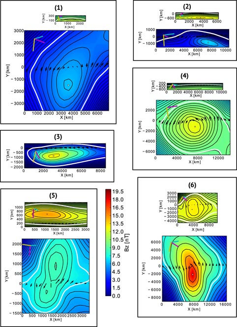
Figure 4. GSRs for the six islands. P1 reconstructions are at the top of each box and P2 at the bottom, except for event 3 only P2 is depicted. The Bz maps are perpendicular to the respective invariant axis. The black contour lines show the equipotential levels (A(x, y) = const). The white line indicates the boundary of undisturbed flux rope (the purple dotted lines in figure 3). The dHT intervals correspond to the full width of the reconstructions. The spacecraft trajectory goes through y = 0, and the magnetic field observations are given by the black arrows along the trajectory. The size of P1 and P2 subfigures is scaled to reflect the reconstructed flux rope spatial size. The colored lines at the top left corner of each subfigure indicate the GSM axes: X (cyan), Y (magenta), Z (yellow).
Download figure:
Standard image High-resolution imageAfter a short interval of Earthward flow (VX > 0), P2 encountered unsteady tailward flow, with pulses of steadily increasing amplitude. Embedded in this interval were bipolar perturbations in BZ, which are the characteristic signature of the loop-like fields associated with flux ropes (red trace in figure 1). P1 observed several signatures characteristic of TCRs (dark blue trace in figure 1), as well as flux rope signatures when it was located in the plasma sheet later in the period of interest. In total, P1 and P2 observed at least 12 and 10 clear bipolar signatures respectively. Six of these were seen by both satellites, and are marked by dashed light blue lines and black numbers in figure 3. The dotted light blue lines indicate events that were seen by only one satellite. The purple dotted lines depict the estimates for the boundaries of the unperturbed cores of the flux ropes obtained with the Grad–Shafranov analysis, discussed in section 4.2. (Note that this same interval has been recently analyzed by [41] as well, and that our event 6 also belongs to their dataset.)
For events 1–5, P1 observed a TCR whereas P2 observed the flux rope in the plasma sheet and the associated plasma jet. During event 6, P1 was initially in the lobe, but cut through the flux rope before returning to the lobe. Throughout all the events, BY was positive, indicating the presence of a guide field. BY was amplified during several of the P2 flux rope encounters, and particularly in event 6.
3.1. Plasma parameters
To aid comparisons with simulation and theory, it is useful to establish various plasma parameters. In reconnection simulations, parameters are often scaled according to the inflow magnetic field strength and the current sheet density. The inflow magnetic field corresponds to the lobe magnetic field strength measured by P1, i.e., Binflow = 11.5 nT, and the plasma sheet density is measured by P2, ncs = 0.08 cm−3. From these values we find that the ion gyroperiod
 , the ion inertial length di = c/ωci ∼ 0.13 RE = 830 km, and the Alfvén speed VA(Binflow, ncs) ∼ 890 km s−1. As such we estimate the separation of P1 and P2 in the YZGSM plane to be ∼12 RE ∼ 92 di.
4. Flux rope properties
4.1. Two-spacecraft analysis
The results of the timing analysis applied to the six events are given in table 1. The first four columns display the event number, the time of the event at P2, the tailward speed measured by P2, and the time interval between successive flux ropes. The fifth column converts this time interval into a spatial scale, assuming that the flux rope propagates constantly at the observed speed. The next set of three columns shows the event time at P1, the time interval, and the spatial separation, assuming propagation at the speed observed by P2. The final set of four columns shows the time delay between the measurements at the P1 and P2, their separation in the X and Y directions, and the tilt angle (equation (1)).
Table 1. ARTEMIS observations of the six magnetic islands.
| # | P2 | P1 | 2-sc-timing | ||||||||
|---|---|---|---|---|---|---|---|---|---|---|---|
| Time (UT) | Visl (km s−1 (VA)) | Δti, i+1
 |
Δxi, i+1 (RE(di)) | Time (UT) | Δti, i+1
|
Δxi, i+1 (RE(di)) | Δtsc (s) | ΔXsc (RE) | ΔYsc (RE) | θ2sc (°) | |
| 1 | 09 : 55 : 16 | −282 (−0.31) | 550 (97) | 19.6 (155) | 09 : 55 : 28 | 624 (110) | 22.3 (176) | 12 | −6.38 | 11.78 | −26 |
| 2 | 10 : 04 : 26 | −227 (−0.26) | 443 (78) | 16.9 (133) | 10 : 05 : 52 | 402 (71) | 15.3 (121) | 86 | −6.36 | 11.74 | −16 |
| 3 | 10 : 11 : 49 | −243 (−0.27) | 494 (87) | 29.9 (237) | 10 : 12 : 34 | 505 (89) | 30.6 (242) | 45 | −6.34 | 11.73 | −22 |
| 4 | 10 : 20 : 03 | −386 (−0.43) | 220 (39) | 13.9 (110) | 10 : 20 : 59 | 215 (38) | 13.6 (108) | 56 | −6.32 | 11.71 | −14 |
| 5 | 10 : 23 : 43 | −403 (−0.45) | 930 (163) | 89.2 (706) | 10 : 24 : 34 | 851 (149) | 81.6 (646) | 51 | −6.31 | 11.70 | −15 |
| 6 | 10 : 39 : 13 | −611 (−0.69) | 10 : 38 : 45 | −28 | −6.28 | 11.68 | −38 | ||||
The tailward velocities of the islands, as measured by P2 in/near the plasma sheet, vary between 230 and 610 km s−1. The speed increases from one island to the next similar to previous observations (e.g., [31]). During this same interval, the properties of the inflow region (as can be estimated from P1 measurements in the lobe) were steady. Accordingly, the outflow velocity increased from 26–31% to ∼70% of the Alfvén speed. As a consequence of the increasing speed, if we assume that the flux ropes maintain a constant velocity as they subsequently travel away from the Earth, flux rope 5 will eventually catch and interact with the previous, slower ones in the distant tail.
The temporal separations of the six events of interest vary from ∼220 to ∼930 s, i.e., from 38 to 163 ion gyroperiods. If we consider flux rope i + 1 at the time when ARTEMIS P2 saw rope i, the spatial separation for the first five islands was ∼20 RE (∼150 di). Given spatial separations as large as this, and the observation location at XGSM > −60 RE, the islands cannot result from a single, pre-existing multi-X-line reconnection region convecting past the spacecraft and it is therefore most likely that these islands were released sequentially.
For island 6, we note that if it had existed at the time of observation of island 5, and had a constant velocity of 610 km s−1, it would have been located at XGSM ∼ 30 RE (on the dayside). We thus conclude that it was probably created later than 10 : 24 UT. Assuming it was formed at the near-Earth neutral line at XGSM ∼ −25 RE [42], the release time would have been around 10 : 33–10 : 34 UT.
4.2. Grad–Shafranov analysis
The Grad–Shafranov analysis was applied to each of the six events at each spacecraft. The reconstructed cross-sections are shown in figure 4, while the numerical results are given in table 2. For most of the events there was almost no ambiguity in determination of the invariant axis direction. The Grad–Shafranov reconstruction (GSR) residual maps were all of similar, reasonable quality, which means that residues between plasma and magnetic field properties in the front and rear parts of the structures were small and similar from event to event [39]; thus we expect no significant differences in error of the invariant axis determination in our event list. The main quality differences were between the two spacecraft due to their different plasma regions and impact parameters [40]: the de Hoffmann–Teller velocities for P2 were very good (〈cc〉 = 0.95) and similar to the observed island velocities. In contrast, it was not possible to find a perfect de Hoffmann–Teller frame for P1 (〈cc〉 = 0.60), so not all the electric fields were eliminated in the reconstruction frame. This is most likely due to P1 being located in the lobe and observing TCR-type signatures; as the flux rope moves past in the plasma sheet, it pushes the lobe plasma resulting in residual, non-unidirectional motion. For P1, we also calculated the reconstruction with magnetic field data alone (as the plasma beta was small), and the results are very similar. We did not do a P1 fit for event 3 as the magnetic perturbation was too weak.
Table 2. GSRs for the six magnetic islands.
| # | P2 | P1 | ||||||
|---|---|---|---|---|---|---|---|---|
| cc | Axis [X, Y, Z]GSM | θGS (°) | αGS (°) | cc | Axis [X, Y, Z]GSM | θGS (°) | αGS (°) | |
| 1 | 0.985 | [−0.748, 0.571, −0.339] | −53 | −31 | 0.592 | [−0.751, 0.624, 0.215] | −50 | 19 |
| 2 | 0.937 | [−0.315, 0.928, −0.200] | −19 | −12 | 0.441 | [−0.741, 0.566, 0.362] | −53 | 33 |
| 3 | 0.930 | [−0.349, 0.791, −0.503] | −24 | −32 | — | — | — | — |
| 4 | 0.971 | [−0.938, 0.346, −0.028] | −70 | −5 | 0.512 | [−0.600, 0.622, −0.503] | −44 | −39 |
| 5 | 0.920 | [−0.824, −0.091, −0.560] | −96 | −99 | 0.594 | [−0.881, 0.184, −0.437] | −78 | −67 |
| 6 | 0.960 | [−0.690, 0.618, −0.378] | −48 | −32 | 0.834 | [−0.847, 0.445, −0.292] | −62 | −33 |
The Bz maps in figure 4 have been scaled for each event (1–6) to reflect the reconstructed flux rope diameters. The P1 reconstructions are slightly smaller than those for P2, though this is probably an effect of crossing TCRs instead of islands (note also the shape of the reconstructions, especially for the events 1, 2 and 4). The first three events were similar in size, 7000–10 000 km (∼10 di). Event 4 was bigger (13 000 km; 16 di) while event 5 was very small (and perturbed) compared to the rest, only ∼3000 km (∼4 di). Note also that for P2 measurements of event 5 the GSR estimated undisturbed flux rope boundary (white contour in figure 4, purple dotted lines in figure 3) does not match the visual identification of the bipolar BZ variation. Flux rope 6 was clearly the largest one, about five times bigger in diameter than event 5. Overall, the GSR diameters are similar to those seen in 3D PIC simulations [26, 27]. The common color-scale in figure 4 facilitates the comparison of the reconstructed core magnetic field strengths. We can see that the field strength varied between ∼7 and ∼14 nT for the first five events, while the sixth had a larger core field of ∼19 nT.
4.3. Combined picture of orientation and curvature
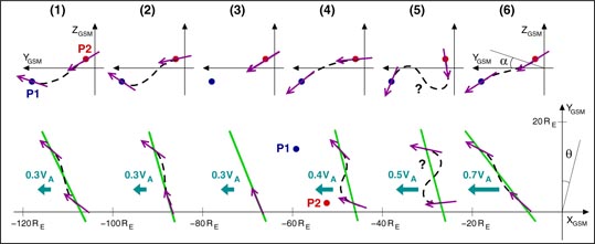
We now consider the orientation and curvature of the flux ropes using both the two-spacecraft-timing analysis (section 2.2.1) and the results of the GSR analysis (section 2.2.2). To calculate the tilt angle θ2sc of each flux rope (equation (1)), we use the P2 VX measurements and assume that the flux rope propagates at a constant speed. The results of the two-spacecraft-timing are given in the last column of table 1. The tilt angles for the first five ropes vary between −14° and −26°, while the last one had a larger tilt of −38°. Overall, the orientations are rather well organized and consistent. The sign of the angle indicates that the end of the flux rope on the dusk flank (YGSM > 0) is leading, with the dawn flank (YGSM < 0) trailing.
Figure 5 shows the six events as projections in the YZGSM (top) and XYGSM (bottom) planes. This figure is drawn to scale, except that the separation in XGSM is set to a constant value. The green lines (bottom) give the two-spacecraft-timing axis orientation (table 1, column 12). The purple arrows give the GSR invariant axis directions. The dashed line illustrates the inferred curvature, obtained by connecting the observed axis directions. For events 1, 2, 3 and 6 the local GSR axes are reasonably close to the global XY orientation inferred from the two-spacecraft-timing, and can be interpreted to represent smaller scale undulations in the axis orientation. For events 4 and 5, the GSR axes differ significantly from the global orientation, even though the quality of the fit (ccs in table 2) is similar.
Figure 5. Cartoon illustrating the observed relative orientations of the islands in YZGSM (top) and XYGSM (bottom) planes. The figure is drawn to scale, except that the separation in XGSM is set to a constant value. The spacecraft location are depicted by the blue (P1) and the red (P2) dots. The green lines (bottom) show the two-spacecraft-timing axis orientation (θ2sc), while the purple arrows give the GSR invariant axis directions (θGS and αGS). The dashed lines illustrate the inferred curvature. The light blue arrows indicate the flux rope speed measured by P2.
Download figure:
Standard image High-resolution image
The top row of figure 5 shows the GSR estimates in the YZGSM plane (αGS in table 2), looking from the tail toward the Earth. The arrows are placed at the satellite location because the impact parameters (figure 4) tend to be underestimated. The dashed lines indicate again the inferred curvature. Note that the orientation is such that higher end (P2) has to connect (if it still is connected) to the South pole and the lower end (P1) to the North pole, implying a twist closer to Earth. Event 5 seems very disturbed, if the P1 and P2 observations correspond to a single flux rope and the GSR results are applicable.
5. Discussion
The data show that the two ARTEMIS satellites observed a series of flux ropes, stretching more than 10 RE (90 di) in the out-of-plane direction. Both dual- and single-spacecraft methods show that the flux ropes were tilted (−38° < θ < −14°), all in the same direction. Previously, the single spacecraft statistical study of 73 flux ropes by [5] indicated a very large variability in the tilt angles, covering basically all directions in the XYGSM plane. In a more recent ARTEMIS study with a small separation in the out-of-the-reconnection-plane direction (ΔYGSM ∼ 3 RE), [31] used single-spacecraft methods to infer the axis direction of three flux ropes. They found tilt angles θ ∼ +45°, i.e., similar to the values reported here, but of opposite sign (dawn-end leading).
Two recent 3D PIC simulations have addressed the formation of flux ropes: [26] studied the case of very large guide field (90° magnetic shear) in a long simulation run (tΩci = 98), while [27] considered the initial stages (tΩci = 4.8) of both anti-parallel and small guide field (a third of the asymptotic magnetic field) reconnection. In both ARTEMIS studies the observed tilt angles are larger than in [26], but this is perhaps due to simulation's larger guide field. The parameters in [27] are closer to the magnetotail ones, but at such early stages (and at 10 di azimuthal scales) the flux rope orientation and kinking seemed to be mainly driven by coalescence.
The global scale orientation reported here may be due to two different scenarios: (i) the islands were parallel to the X-line, but the X-line was tilted with respect to YGSM axis, or (ii) the islands were tilted with respect to the X-line that was parallel to the YGSM axis. In the first scenario the island would be released simultaneously along the X-line, and the outflow velocity had to be oblique, not orthogonal, with respect to the X-line in order to be consistent with the observed plasma flow along the XGSM axis. Simulations (e.g., [21]) indicate that the jet is tilted toward the current direction due to Hall effects, which is in agreement with the magnetotail (ion) current direction (+YGSM). The second scenario implies that each flux rope grew (and was subsequently expelled from the X-line) in the −YGSM direction, i.e., the direction of the electron current. We find this scenario more plausible, as the simultaneous island appearance and release over a 92 di distance seems unlikely. We find that this cycle repeats on a time scale of the order of 100 ion cyclotron periods, although table 1 shows that there can be significant variation around this characteristic time. Interestingly, the observed outflow speed increased significantly from one rope to the next, while the angle stayed similar for the first five events, implying that the island spreading speed increased at the same rate.
The formation of the islands is related to the associated X-line's growth speed and direction, which are governed by the strength of the guide field and the nature of the current carriers [22]. For the magnetotail, some studies indicate electrons to be the main current carriers [23, 24], while others point to ions in the YGSM > 0 region [25]. On-going simulations suggest that the islands grow in the direction opposite to the X-line spreading direction [43], implying that in our scenario (ii), the X-line spread in the ion current direction (+YGSM).
The structure of the flux ropes showed clear evolution within the chain. The first flux ropes were rather linear, given the good correspondence of the local (GSR) axis orientation with the global orientation (two-spacecraft-timing). However, by events 4 and 5 (10 : 24 UT; 260–310  from event 1) either (a) the secondary islands became very disturbed/kinked or (b) the size of the islands became less than the spacecraft separation (∼90 di; i.e., the spacecraft may have seen two different islands at the same time). Flux ropes are subject to kink instability, where the axis itself develops a helical structure. Open-ended ropes have been found to be more unstable than ropes anchored at both ends (e.g., flux ropes rooted in the solar surface) [44]. As there is a significant difference between the global and local axis orientations for events 4 and 5, we infer that such kinking may be present; indeed, the GSR axes of events 4 and 5 can be fitted with a left or right handed helical axis. Yet without a global kinetic simulation of the magnetotail, it is difficult to say if this is truly the case. Nevertheless, we note that in full 3D PIC simulations, the flux ropes suggest some kinking already at tΩci = 4.8 in [27], while very turbulent structure is reached by tΩci = 98 in [26]. It would be of interest to examine such simulations in more detail to establish whether, for example, the kink instability develops in secondary islands at late stages of the evolution.
Throughout the analysis we have found that event 6 had different properties compared to the evolution of the rest of the chain: it had consistently larger tilt in the XYGSM plane and a bigger core field and cross-section. It was also a rather straight rope similar to the first events of the chain. Event 6 was probably created around 10 : 33–10 : 34 UT (propagating back to XGSM ∼ −25 RE with constant speed). Placing this in a geophysical context, the AE index increased during events 1–5 peaking at 1050 nT at 10 : 24 and 10 : 28 UT (strong substorm activity), but then dropped sharply, signaling the beginning of a substorm recovery phase. This coincided with/was followed by a northward turning of the Interplanetary Magnetic Field according to upstream solar wind observations (ACE and Wind spacecraft). As such, we suggest that flux rope 6 might correspond to a new reconnection X-line, as the solar wind conditions changed around/between events 5 and 6, and that the different properties are related to the new boundary conditions.
6. Conclusions
Magnetic flux ropes are a common feature of magnetic reconnection in the Earth's magnetotail. Here we have analyzed in detail six flux ropes that were part of a chain of tailward moving events observed by the two ARTEMIS satellites. The two satellites were separated by more than 10 RE (90 di) in the YGSM direction, allowing the three-dimensional structure and orientation of the flux ropes to be explored.
The analysis shows that the six flux ropes were released sequentially, and therefore were most likely produced by a secondary instability at the X-line. The speed of the flux ropes increased from ∼0.3 VA to ∼0.7 VA, which has been seen previously but here we show the speed increase from one rope to another in terms of the Alfvén speed. Both global timing analysis and local Grad–Shafranov analysis show that the flux ropes were consistently tilted in the XYGSM plane, with first five events exhibiting a tilt of ∼20° (dusk-end leading). This tilt is qualitatively consistent with the growth of the secondary instability along the direction of electron current (the −YGSM direction). The first flux ropes were linear while later ones appeared twisted. The sixth event had a larger tilt of ∼38°, and also larger core field and a larger cross-section. Based on the geophysical context, including a change in the solar wind input and the start of a recovery phase of a geomagnetic substorm, we conclude that this event may correspond to the creation of a new X-line or significant disruption of the existing X-line.
Acknowledgments
We acknowledge NASA contract NAS5–02099 for use of data from the THEMIS Mission. The work of HH and JPE is funded by the UK Science and Technology Facilities Council (STFC); JPE holds an STFC Advanced Fellowship at Imperial College London. The Alfred Kordelin foundation is also thanked for financial support. HH acknowledges fruitful discussions within the international team lead by T Phan at the International Space Science Institute (ISSI) in Bern.