Abstract
Merging-compression start-up in the Mega Ampere Spherical Tokamak provides an opportunity to investigate the merging of flux ropes through magnetic reconnection, and the self-organization into a single flux rope, in a low-plasma-β, high-Lundquist-number plasma. We present an overview of simulations of this process using the compressible Hall-MHD equations in two dimensions. Preliminary results of an analytical model of the self-organization, assuming a helicity-conserving relaxation to a minimum energy state, are also presented. The relevance of these models to solar plasmas is discussed.
Export citation and abstract BibTeX RIS

Content from this work may be used under the terms of the Creative Commons Attribution 3.0 licence. Any further distribution of this work must maintain attribution to the author(s) and the title of the work, journal citation and DOI.
1. Introduction
Magnetic reconnection is a process for re-structuring magnetic fields and dissipating free magnetic energy which is of importance in a wide range of space and astrophysical plasmas, as well as magnetically-confined fusion plasmas in the laboratory [1–3]. Magnetic flux ropes are a basic building block of magnetic fields, and the merging of flux ropes through magnetic reconnection is a frequently-occurring process. Considerable understanding of flux-rope merging has been attained through purpose-built laboratory experiments e.g. [4–10].
Here, we report on the modelling of flux-rope merging in the Mega Ampere Spherical Tokamak (MAST), which is in a parameter regime more closely resembling astrophysical plasmas. MAST [11–13] is a tight-aspect ratio toroidal device, in which plasmas are created with typical major and minor radii R = 0.95 m, a = 0.60 m, plasma current Ip = 400–900 kA, toroidal field at the magnetic axis BT = 0.40–0.58 T, and peak electron density and temperature ne0 = 3 × 10¹⁹ m−3 and Te0 = 1 keV. The MAST device has demonstrated the very promising potential of the spherical tokamak as a fusion power plant or Component Test Facility, especially in terms of confinement and high β operation, as well as providing insight into a range of physical processes relevant to conventional tokamaks. Several alternative plasma start-up methods can be used to reach these final parameter values, one of which is the merging-compression technique, whereby two flux ropes with parallel toroidal current move towards each other and then merge, forming a plasma torus with a single set of closed magnetic flux surfaces [2]. In addition to being an attractive scheme for plasma start-up and current drive without the use of a central solenoid, merging-compression in MAST also provides an opportunity to investigate the basic physics of flux-rope merging and magnetic reconnection in conditions of higher Lundquist number and lower plasma beta than those of other laboratory experiments, and in parameter regimes more closely resembling those of at least some astrophysical plasmas, such as the flaring solar corona. Moreover MAST is equipped with a comprehensive set of diagnostics, including Thomson scattering lasers (see right-hand frame of figure 1) that make it possible to obtain electron temperature and density profiles with sufficiently high time resolution to study the dynamics of reconnection during the merging process.

Figure 1. A cartoon of merging-compression formation in MAST [13, 17], with the flux ropes shown in purple. The poloidal cross-section is shown (R horizontal, z vertical). The left-hand panel shows the initial stages, when the flux ropes form around the P3 poloidal field coils. The right-hand panel displays the flux ropes on the point of merging, showing also the location of Thomson scattering line-of-sight where density and temperature measurements are taken. Reproduced with permission from [17]. Copyright 2013 The American Institute of Physics.
Download figure:
Standard image High-resolution imageThe merging-compression formation scheme was pioneered on MAST's smaller predecessor START [14]. In this scenario, described more fully by [15–17], two toroidal flux ropes with parallel toroidal currents are produced around in-vessel poloidal field coils (the P3 coils shown in figure 1). Decreasing the current in the coils induces plasma current in the flux ropes and causes them to separate from the coils, mutually attracting due to their parallel currents; they eventually merge through reconnection of the poloidal field at the midplane (see figure 1). The process presently generates spherical tokamak plasmas with a current of up to 0.5 MA, which are rapidly heated (presumably, mainly by processes associated with the reconnection) to temperatures of up to 1 keV.
In section 2, we present an overview of recent numerical simulations of merging-compression in MAST using both resistive magnetohydrodynamic (MHD) and Hall-MHD equations, with the HiFi modelling framework [18, 19]. These are performed in 2D, both in Cartesian geometry and in tight-aspect ratio toroidal geometry; for more details, see [17]. Then, in section 3, we describe initial results from an analytical model explaining the self-organization of the flux ropes in terms of a helicity-conserving relaxation to a minimum energy state. Conclusions are presented, and the relevance for astrophysical plasmas is discussed, in section 4.
2. Resistive MHD and Hall-MHD simulations
Here, we describe results of simulations using both single-fluid MHD and Hall-MHD. The Hall terms in Ohm's law are included here because, for typical MAST parameters (see below), the ion skin-depth is comparable with the device size (normalized di = 0.145) and is much larger than the width of the Sweet–Parker current sheet predicted by resistive MHD. A hyper-resistive term [1] representing anomalous electron viscosity due to effects of micro-turbulence and 3D instabilities is also included, which sets a dissipation scale for whistler and kinetic Alfvén waves and provides a parallel electric field to allow reconnection in the 2D simulations. Other terms, such as electron inertia and off-diagonal pressure tensor terms, are likely to be less significant, but will be included in future modelling. We solve the nonlinear compressible Hall-MHD equations in normalized form [1]. The normalization is with respect to typical MAST start-up plasma values: density n0 = 5 × 10¹⁸ m−3, length-scale L0 = 1 m, magnetic field B0 = 0.5 T, and (equal) ion and electron temperatures T0 = 10 eV. Velocities are normalized by the Alfvén speed v0 = B0 (μ0n0mi)−1/2. The full set of equations is


where n is the density, j = ∇ × B the current density, vi the ion velocity (with electron velocity ve = vi − di j/n), B the magnetic field, p = pi + pe the total (sum of the ion and electron) thermal pressure, E the electric field and A the magnetic vector potential. The ion stress tensor is
 , and the heat-flux vector q has anisotropic form
 where
where
 . The coefficients are: normalized ion skin-depth,
 , resistivity in terms of the parallel Spitzer value η = (μ0v0L0)−1ηSp,∥, hyper-resistivity ηH, viscosity
 , and the normalized parallel electron,
 , and perpendicular ion,
 , heat conductivities; here, we set the normalized values to be
 and
and
 . The final term in equation (3) is the hyper-resistive diffusion. On the basis of Braginskii values based on pre-merging MAST temperatures, η = 10−5 and μi = 10−3; but the values of η, μi and ηH are also sometimes varied in order to study the scaling effects of collisions on the merging. With these standard values, the Lundquist number S = 105 and the magnetic Prandtl number Pm = 100.
The simulations use a grid with NR = 180, Nz = 360 finite elements in the R, z directions, with a polynomial of order 4 in each element, giving an effective resolution of 720 × 1440. The spacing is non-uniform, with a finer grid near the current sheet location around z = 0. Convergence studies have been undertaken.
The initial conditions are taken as two localized distributions of toroidal current representing the plasma when the current rings have detached from the in-vessel coils (which are not modelled). The toroidal field within the flux ropes is calculated so as to give local force-balance, but an attractive force between the parallel currents remains and triggers the merging process.
Figure 2 shows a sequence of fields for a resistive MHD simulation (di = 0, ηH = 0; η = 10−5, μ = 10−3), in Cartesian geometry. It can be seen that as the flux ropes approach, a current sheet initially forms, which becomes the site of reconnection. The pile-up of the poloidal field (BR), associated with a layer of reverse toroidal current (see second panel of figure 2), opposes the merging and causes the reconnection to stall. This process continues, leading to oscillations in the reconnection rate or 'sloshing' [20, 21] which can be seen in some traces on figure 3. The 'sloshing' is known to occur for sufficiently small values of η, and can be interpreted as being due to the increase in induced current between approaching magnetic islands, on a timescale more rapid than resistive decay, leading to a repulsive force [22]; thus, the frequency scales with the Alfven time. Nevertheless, full merging of the flux ropes is eventually achieved, as shown in the final panel of figure 2. For the resistive MHD case, analysis of the scalings with μ and η [17] shows that the reconnection rate is consistent with the visco-resistive Sweet–Parker reconnection [23, 24].
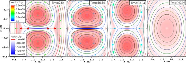
Figure 2. A series of snapshots showing poloidal field (contours), toroidal current density (colour scale) and poloidal ion velocity (arrows) from a resistive MHD simulation. There is also a toroidal (out of plane) field component, so these plots represent slices through twisted flux ropes. Note the region of flux-rope interaction is shown, which is smaller than the full simulation box.
Download figure:
Standard image High-resolution image
Figure 3. The time dependence of reconnection rate for hyper-resistive Hall-MHD simulations with varying hyper-resistivity, ηH and di = 0.145. For comparison, a MHD simulation (di = 0) with hyper-resistivity is also shown (black line). In all cases η = 10−5, μi = 10−3.
Download figure:
Standard image High-resolution imageThe time dependence of the reconnection rate for Hall-MHD is shown in figure 3, along with a comparable single-fluid MHD case in which the hyper-resistivity has been included, in order to distinguish between the effects of finite ion skin-depth and hyper-resistive diffusion. Note that the reconnection rate for the single-fluid case, with hyper-resistivity—performed largely as a numerical test of the effects of hyper-resistivity—is very close to that for resistive MHD, since the breaking of the frozen-in condition is largely provided by the resistivity η at this low value of ηH = 10−10). Evidently, inclusion of the Hall terms in Ohm's law can significantly increase the reconnection rate. As the hyper-resistivity decreases from 10−6 to 10−7, both peak and average reconnection rates decrease; as ηH approaches 10−10, the peak reconnection rate becomes larger (see below). Note that the contribution to the reconnection electric field by the hyper-resistivity dominates over the resistive contribution for the Hall-MHD simulations.
The structure of the reconnection region also changes significantly as the Hall terms are included: the symmetry is broken, leading to a tilted current sheet and tilted ion outflow jets [17]. The effects of varying collisionality are explored by changing the hyper-resistivity ηH [17], showing a transition between various reconnection regimes. For higher collisionality, ηH = 10−6, a broad current sheet forms which does not fragment. Reducing the collisionality leads to break-up of the sheet due to tearing-type instabilities. At low values of ηH, the thin current sheet becomes unstable to secondary island formation, and a series of small islands (regions of closed magnetic flux) are generated, separated by additional X-points; see figure 4. At the lowest values simulated, ηH = 10−10, the current sheet spreads asymmetrically across the separatrix between open and closed flux, and the outflow region opens, leading to fast reconnection.

Figure 4. Poloidal flux contours and current density (in colour-scale) during reconnection for a Hall-MHD simulation with normalized ηH = 10−9, showing the formation and ejection of magnetic islands.
Download figure:
Standard image High-resolution imageSimulations have also been performed in tight-aspect-ratio toroidal geometry, with a confining vertical field in addition to the dominant toroidal field (with 1/r dependence), more closely representing MAST. The flux-rope merging proceeds as before, leading to the formation of a single 'spherical tokamak' state with closed flux surfaces and a realistic, monotonically-increasing profile of the safety factor q, with q > 1 everywhere. There are some differences in the dynamics from the Cartesian case, especially due to the inboard-outboard asymmetry; in particular, the islands which form in the current sheet are more easily ejected. For further details, see [17, 25].
The simulations also predict the plasma density profiles. It has been shown that, in the case of Hall-MHD simulations in toroidal geometry, a double-peaked radial density structure in the midplane is predicted, which agrees with experimental measurements using Thomson scattering [15, 17]. This is discussed in more detail in [17], where it is shown that explaining the observed double-peaked density structure requires both two-fluid and toroidal effects.
3. Relaxation model and self-organization
The concept of helicity-conserving relaxation to a minimum energy state was pioneered for reverse field pinch plasmas by Taylor [26] and has subsequently been applied with great success in a range of a laboratory plasmas (see review [27]) as well as astrophysical plasmas such as the solar corona (e.g. [28, 29]). The basic idea is that a plasma subject to some initial disturbance or instability relaxes towards the state of lowest magnetic energy, with the constraint that the total magnetic helicity is conserved. The latter constraint is appropriate in a highly-conducting plasma in which dissipation is mostly due to reconnection within thin current layers; the basic idea is that reconnection enhances energy dissipation, but not helicity dissipation (whilst both slowly dissipate due to global resistive diffusion) [27, 30]. In this case, the relaxed state is a linear force-free field,

where μ = μ0B · j/B2 is spatially constant.
We propose, following an earlier suggestion for START (M Bevir and C G Gimblett, private communication), that flux-rope merging in MAST can be modelled as a Taylor relaxation. Initial results of such a model are presented here; for simplicity, a Cartesian geometry is assumed, with a rectangular cross-section infinite-aspect ratio tokamak ('toroidal' invariant direction z). The model could be easily adapted to a tight-aspect-ratio system in cylindrical geometry, following [31]; but, as demonstrated by the numerical simulations in section 2, this should not have a major effect on the results. Furthermore, the aim of the relaxation model is to draw out some essential underlying physics, and this would not be greatly enhanced by a more accurate choice of geometry.
3.1. Relaxation model
The initial state, shown in the left-hand panel of figure 5, consists of two adjacent, twisted flux ropes, with square outer cross-sections given by x = 0, a (for both flux ropes) and y = 0, a for one flux-rope and y = a, 2a for the other; hence, the flux ropes touch along the surface y = a. We assume each initial flux rope is force-free. The field then undergoes helicity-conserving relaxation to a single flux rope contained within the same overall volume (0 ⩽ x ⩽ a; 0 ⩽ y ⩽ 2a). The relaxed state is described by (6). For ease of calculation, we assume that the initial flux ropes are individually linear force-free fields, also described by (6); there is no particular reason to assume such a μ profile, but as we have no detailed knowledge of the current distribution, this is not unreasonable (note therefore that the initial current profile here is somewhat different from that in section 2). However, the initial state is not a minimum energy state, because it contains a current sheet at the boundary between the two flux ropes (at y = a), due to the discontinuity in the poloidal field Bx which reverses direction. Hence the model initial state represents the fields at the point in time at which the flux ropes have been brought together by the attractive force, but have not yet commenced reconnection (somewhat later than the initial state of the simulations). This is a force-free equilibrium, since the magnetic pressure balances (by symmetry) across the interface y = 0; but is not a relaxed (constant-μ) state because μ has a negative value, with delta-function dependence, in the current sheet.

Figure 5. Poloidal fieldlines for initial and final states for the relaxation model of merging; distances are normalized with respect to the width a. The initial field (left) has μia = 1.25. The final field (right) has μfa = 0.782. In both cases, there is also a toroidal field (BZ = μψ), so that closed poloidal flux contours correspond to twisted magnetic flux ropes.
Download figure:
Standard image High-resolution imageThe fields for the general case of a rectangular boundary a × b are found using a flux function ψ, where B = (∂ψ/∂y, −∂ψ/∂x, μψ), so (6) leads to

The boundary condition is ψ = ψb = constant on the boundary, where ψb, which is effectively a normalization constant for the fields, must be non-zero. With the choice Bz = μψ made above, with the allowable arbitrary constant set to zero, this is equivalent to requiring non-zero toroidal field on the boundary. (For ψb = 0, the only non-trivial solutions to (7) are spheromak-like solutions for discrete eigenvalues of μ, which are not relevant to spherical tokamaks). Following [32] and [31], the solution is expressed as

which automatically satisfies the required boundary condition. Substitution into (7) gives
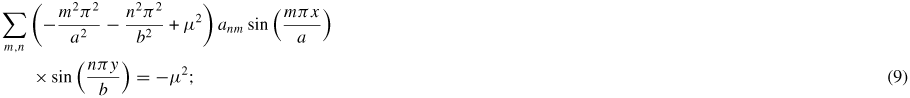
using the orthogonality of the eigenfunctions, sin (mπ x/a) sin (nπy/b), within the summation then yields


see also [33]. Results are presented in dimensionless form with lengths scaled with respect to a. We also normalize so that the toroidal flux Φt ≡ ∫ABz dx dy = 1 (thereby ensuring conservation of flux during the relaxation process described below), so that ψb is a function of μ. It should be noted that, with this normalization, ψb, and all related quantities such as energy and helicity, diverge as μ approaches the first eigenvalue of (7) [32, 34]; however, since we are interested here in tokamak-like magnetic configurations with strong toroidal fields, this occurs outside the relevant parameter range.
The fields from (8), (10) are used both to represent the individual flux ropes in the initial state (with b = a) and the single relaxed state (with b = 2a). The final value of μ, μf, is determined from the initial value by the constraint that helicity, K, and total toroidal flux are conserved (where the dimensionless total toroidal flux initially is 2, because of the two flux ropes). A root-finding process is used to find μf so as to conserve
 . The helicity is given by

where we fix Az = 0 on the boundary so that the gauge-correction term arising from the flux through the torus [35] vanishes. It can be shown that this is related to the total magnetic energy, W, by

where the energy (per unit length) is obtained by integration of the fields, as

where ψb(μ, a, b) is given by the normalization Φt = 1 (and μ0 = 1 in dimensionless units).
3.2. Relaxation results
A typical relaxed state is shown in the right-hand panel of figure 5. Note that this represents the post-merging state, and is indeed very similar to the final states of the numerical simulations as shown in figure 2.
The energy released during relaxation is calculated as ΔW = Wi−Wf where the initial energy Wi = 2W(μi;a, a) and the final energy is Wf = 4W(μf;a, 2a) (the factors 2 and 4 are to account for, respectively, two flux ropes with Φt = 1 initially, and a single flux rope with Φt = 2 finally. In figure 6, the final value of μ is plotted against the initial value, as well as the non-dimensionalized energy release ΔW.
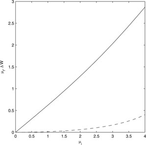
Figure 6. Final μ = μf (solid curve) and energy released, ΔW (dashed curve), as a function of the initial value μi (dimensionless units), for the relaxation model.
Download figure:
Standard image High-resolution imageSince the toroidal plasma current is It = μΦt, figure 6 may also be interpreted, re-scaling the axes by the appropriate μ values, as showing the dependence of final plasma current on initial current (in one flux rope). However, the initial state also includes a current sheet, and in order to calculate the total initial plasma current, we must add the (negative) net current in this sheet, which may be simply obtained as
 .
.
It can be shown analytically that for small μi,
 , μf ∼ μi. Hence the final plasma current depends linearly on the initial current; whilst the energy release depends quadratically on μi. The dependence of μf on μi shown in figure 6 appears as a straight line, but the scaling is in fact stronger than linear; for larger μi, approaching the first eigenvalue, the linearity clearly breaks down.
As shown in section 2, the magnetic energy released by reconnection may both heat the plasma and drive plasma flows—but the latter may also be dissipated to provide further heating. We obtain an estimate (strictly an upper bound) on the temperature increase—here simply within single-fluid MHD—by assuming that the released magnetic energy is converted fully into thermal energy. For illustration with typical MAST parameters, we take a = 0.4 m and Bt = 0.5 T ⇒ Φt = 0.08 Wb. Taking
 gives
gives
 (here, an asterisk denotes dimensionless quantities), leading to a total initial plasma current of 300 kA, compatible with experiment and the modelling described above (but with somewhat larger currents in the plasma rings). The energy release is ΔW* = 0.0022, which, equating to the thermal energy (3/2)(2n)kT (2a2) gives a temperature rise of about 150 eV, which is compatible with what is experimentally observed—of course, the relaxation model cannot predict any spatial distribution of temperature. Note that the temperature increase depends (to a very good approximation) quadratically on μi and hence on the initial plasma current and on the pre-merger poloidal field, in agreement with experiment [15].
3.3. Comparison of relaxation model with numerical simulations
As noted above, the relaxation model captures the self-organization of two flux ropes into a single one, and the predicted relaxed state is in very good qualitative agreement with the final state of the simulations (comparing final panels of figures 2 and 5). As a further test, we calculate the time evolution of magnetic helicity (see equation (12) as well as the magnetic, kinetic and internal energies, in the resistive MHD simulation simialr to that described in section 2. This is shown in figure 7. The helicity is indeed subject to global resistive diffusion and decays, as expected; however, the helicity evolution is seen to be insensitive to the dynamics of the reconnection and shows no sign of the 'sloshing' oscillations which are evident in the energy traces. The energy traces show that the reconnection causes an increase in kinetic energy (associated with reconnection outflows), while the magnetic energy falls. The semi-oscillatory nature of the reconnection is clearly seen in all the energy traces, but most clearly in the kinetic energy. Note also that, in agreement with the relaxation picture, the kinetic energy eventually falls to a very low value, so that most of the dissipated magnetic energy is converted into thermal energy.

Figure 7. Time evolution of normalized helicity and energies for the resistive MHD numerical simulation with η = 10−5, μi = 10−4, ηH = 0. (a) Helicity. (b) Magnetic energy. (c) Thermal energy. (d) Kinetic energy.
Download figure:
Standard image High-resolution image
The drop in normalized helicity, about 1.2 × 10⁻³, is somewhat lower than the corresponding drop in magnetic energy, 6.0 × 10⁻³. This is an indication that the magnetic energy release due to reconnection is not strongly dominating over the dissipation due to global Ohmic diffusion. In simulations with multiple reconnection sites, where dissipation due to reconnection is dominant, the disparity between energy and helicity dissipation is much greater [30]. Nevertheless, the relaxation picture still captures the essential features of the final state and the energy conversion. We would also expect the resistive dissipation of helicity to be far lower in more highly-conducting plasmas such as in the solar corona.
4. Conclusions
We have described two approaches to modelling the merging of flux ropes in the MAST device. In both cases, the self-organization through magnetic reconnection of two initial flux ropes into a single flux rope is predicted. Resistive MHD and two-fluid simulations using the HiFI framework, in both 2D Cartesian and toroidal geometries, provide detailed information about the dynamics of the reconnection process and its dependence on the collisionality and other parameters. A simple analytical model based on Taylor relaxation theory captures some aspects of the self-organization, predicting the final field state and the plasma heating for given initial conditions.
The numerical simulations presented here are all in 2D. The relaxation model could in principle account for a non-axisymmetric relaxed state, but this would only be attained for far higher values of μ than are relevant here [26, 27]. The twisted flux ropes have strong toroidal fields (typically 5 times the poloidal field), and hence are very unlikely to be subject to kink instabilities. The final state of the simulations also has q > 1 everywhere, indicating stability. (Note that the stability will depend also on the aspect ratio, which is larger for the initial individual flux ropes than for the final state.) Nevertheless, there may be some interest in considering 3D effects in future, particularly on the post-merger evolution, where experimental results sometimes indicate the development of non-axisymmetric structure.
One motivation for studying reconnection in MAST is the relevance to astrophysical and space plasmas. In the solar corona, reconnection occurs with dramatic consequences in solar flares, as well as being likely to contribute to the overall heating of the coronal plasma, and occurring frequently during emergence of flux ropes from the interior. A comparison between MAST and coronal parameters is shown in table 1. Whilst the coronal value of the Lundquist number S, at least on global scales, is very much larger than the MAST value, MAST has a higher S than any other currently operating laboratory reconnection experiment [15]. Coronal reconnection is widely modelled using single-fluid MHD. However, the predicted length-scales of reconnecting current sheets in solar flares are comparable with the ion skin-depth, provided that the dissipation-scale is not anomalously enhanced: thus, Hall terms (at least) should be included and the parameter regime is quite similar to that described here.
Table 1. Table showing comparison of typical values for magnetohydrodynamic variables, dimensionless parameters, non-MHD (two-fluid and kinetic) scales, and current-sheet parameters.
| Quantity | Solar flare | MAST merging-compression |
|---|---|---|
| Typical values | ||
| Global length | L ∼ 107 m | L = 1 m |
| Ion species | Hydrogen | Deuterium |
| Magnetic | B ∼ 0.01 T | Bp = 0.1 T, BT = 0.5 T |
| Temperature | T ∼ 100 eV | T = 10–1000 eV |
| Density | n ∼ 1015 m−3 | n = 5 × 10¹⁸ m−3 |
| Dimensionless | ||
| Plasma-β | β = 10−4–10−2 | βT = 10−4–10−2, |
| βp = 10−3–10−1 | ||
| Lundquist number | S = 1012−14 | S = 104−7 |
| Non-MHD | ||
| Ion skin-depth | di = 10 m | di = 14.5 cm |
| Ion gyro-radius | ρi = 0.1–1 m | ρi = 0.15–1.5 cm |
| Current-sheet | ||
| Sweet–Parker width | δSP = 1–10 m | δSP = 0.03–1 cm |
| δSP/di | 0.1–1 | 0.002–0.07 |
Work is currently in progress to extend the two-fluid simulations to include separate electron and ion temperature distributions, which may be compared with Thomson scattering measurements and ion temperature measurements, where available. It is also planned to explore the effects of changing the initial flux-rope currents. This modelling may also be adapted to study other devices with merging flux ropes.
The relaxation-based model will be extended to toroidal geometry in future. It will also be interesting to investigate further the comparison between the simulation results and the relaxation model, for example, by checking the scalings of heating with plasma current predicted by the latter. It will be particularly interesting to do this both for the resistive MHD and the Hall cases. In the latter case, alternatives to the standard Taylor relaxation approach should also be considered, with additional invariants [36, 37]. The relaxation model may also be easily applied to astrophysical phenomena; in this context, it would be interesting to consider merging and self-organization of multiple flux ropes e.g. [34, 38], with implications for solar coronal heating.
Acknowledgments
This work was funded by STFC, the US DoE Experimental Plasma Research program, the RCUK Energy Programme under grant EP/I501045, and by the European Communities under the Contract of Association between EURATOM and CCFE. The views and opinions expressed herein do not necessarily reflect those of the European Commission. Simulations were run at the Solar-Terrestrial Environment Laboratory (STEL) cluster at Nagoya University,the US National Energy Research Scientific Computing Centre and the St-Andrews MHD cluster funded by STFC. A S would like to thank Kanya Kusano for access to the STEL computer.