


Abstract
In this letter, we find how the frequency of an oscillation determines the exact form of the control for suppressing the oscillation through feedback controls with time delays. These results are based on necessary and sufficient conditions we analytically established for the stability of a dynamical system with feedback control and time delays. We also interpret how these conditions change as the time delay either is equal to zero or becomes larger appropriately. All the analytical and numerical results are illustrated by suppressing the oscillations of the FitzHugh-Nagumo model and by the oscillation death and synchronization phenomena observed in a complex dynamical network with time-delayed couplings. Our findings could be potentially useful for modulating oscillations through proper control devices in various fields.
Export citation and abstract BibTeX RIS
Introduction
Various oscillations are ubiquitously observed in nature and man-made systems. Some oscillations are beneficial; while some others, harmful to the system's stability, need to be suppressed or modulated [1–4]. For example, oscillations observed in gene regulation are in charge of encoding or decoding information [5–7]; however, oscillations emergent synchronously in neural activities may impair brain function, which possibly results into some mental disorders as epilepsy [8–12]. Many control techniques have been developed in the past two decades to suppress chaotic oscillations to unstable equilibria or periodic orbits. These include the OGY method [13, 14], the time-delayed feedback controller [15–19], and the adaptive coupling scheme [20–22], which are the three most efficient techniques. To force periodic oscillations to approach unstable equilibria, the preceding techniques have been of some use [13–16, 20–22]. Typically, a stable and diagonal feedback controller is sufficient to suppress periodic oscillations, which we term as a "common sense".
Due to the physical distance of the signal transmission in various real systems, feedback controllers often meet with time delays [23–25]. However, time delays are able to yield richer dynamical behavior, because of the infinite dimensionality of the dynamical systems induced by time delays [23, 24]. These require us to include time delays influence into the oscillation suppression (OS), and to investigate when the "common sense", mentioned above, is preserved or completely broken. It is worth noting that the original time-delayed feedback controller [15, 16] still needs feedback input without any time delay, which is likely to be impractical for controlling real systems in which a remote transmission of the signal is required.
This letter first gives necessary and sufficient (NS) conditions for OS in a typical dynamical system through feedback control with time delays. Establishing these NS conditions requires an analytical solution of a transcendental characteristic equation with complex-valued coefficients. This is different from the discussion on the conventional equation with real coefficients. Basing on these NS conditions we infer an accurate relation between a successful OS and unstable or asymmetric feedback controls when time delay is considered and the value of oscillation frequency is located in a series of periodically appeared intervals. We also investigate how the established conditions change as the time delay either equals zero or becomes larger appropriately. In addition to OS, since some of those network models can be transformed into a typical dynamical model with particular feedback control and time delays, this work is still useful for illustrating oscillation death (OD) [26, 27] and even synchronization occurs in some complex networks with particular time-delayed couplings [17, 18, 28]. To illustrate the practical usefulness of this work, we finally study OS in the FitzHugh-Nagumo model (FHNM) as well as OD and synchronization phenomena in a complex network with particular time-delayed couplings.
A paradigmatic oscillating model with time-delayed control
To begin, we consider the following paradigmatic dynamical model:

which we call a normal form of the super-critical Hopf bifurcation. As a > 0, eq. (1) is capable of generating a stable periodic oscillation with a minimal period T = 2π/(d + γa) and a radius  . Here, for any given a and γ, the larger the value of the parameter d, the higher the frequency of the stable periodic oscillation. Moreover, the equilibrium z0 = 0 of (1) is an unstable focus for which the eigenvalues of the corresponding linearized matrix around z0 are a ± id (a > 0). Now, the task is to force the periodic oscillation to approach z0 through a linear feedback controller with a time delay. Thus, adding such a controller into (1) yields a controlled model:

where τ∈(0,+∞) is a time delay, keiψ is a control gain taking complex values, and k is the coupling strength. We write the complex state variable as z = x + iy. Then, a linearization of (2) around the equilibrium z0 yields

where the elements in the gain matrix are m = k cos ψ and n = k sin ψ. On the one hand, when ψ (mod π) = 0, i.e., n = 0, the value of the above control gain becomes real and then the gain matrix turns to be diagonal and symmetric. On the other hand, when ψ (mod π) ≠ 0, i.e., n ≠ 0, the gain matrix is asymmetric. In addition, m < 0 corresponds to a stable control; conversely, m > 0 induces an unstable control. Note that for optimal control a real-valued (or symmetric) control gain has been used frequently in the community of control; however, a complex-valued (or asymmetric) gain is rarely taken into account until the appearance of those pioneering studies of the equilibrium stabilization via the conventional time-delayed feedback control in physics [16–19].
Necessary and sufficient conditions for stability
Clearly, a successful suppression of the periodic oscillation in (2) depends on the local stability of the equilibrium z0. Actually this local stability can be determined equivalently by analyzing the root distribution of the characteristic equation of (3):

with respect to λ [23–25]. If the feedback control without time delay is considered, the local stability can be assured by fulfilling the condition m < −a < 0. This is consistent with the "common sense" when τ = 0. However, τ > 0 modifies (4) to a transcendental equation with complex-valued coefficients and infinitely many roots. Although there have been several numerical works on the root distribution including a systematical study with the aid of the Lambert function [16, 29, 30], there are only a few completely analytical results in the literature on NS conditions which practically ensure the location of all the roots of eq. (4) on the left half of the complex plane  for arbitrarily given time delay τ.
In order to establish such NS conditions, we apply the following transformations of the argument and complex parameters:

Here, b = −kτe−aτ and α = ψ − dτ (mod π), so that  and α∈[0,π). Hence, eq. (4) is transformed into:

It can be directly verified that each root of eq. (4) is on the left half of  if and only if [RL]: each root of eq. (5) is on the left side of the line Z = −A in
  , i.e., for any Z0 with h(Z0) = 0, Re{Z0} < −A with A = aτ ⩾ 0.
To analytically give conditions under which [RL] is valid for any τ, we need to describe the root variation along infinitely many branches which are generated by eq. (5) in  for two cases, viz., α ≠ 0 and α = 0. We present our detailed arguments in the Supplementary Information [31]. Here, we summarize in table 1 all the NS conditions on the local stability of the equilibrium z0 for three cases. Case I of our main interest corresponds to the oscillating model (1); however, Cases II, III correspond to a stable z0. The constants in table 1 are illustrated as follows: both α* = α0 and α* = α1 in Case I are the two solutions satisfying the equation

with respect to the argument α*. Here, A = aτ < 1 and y = y*(α*) is the unique solution of the equation 2y = sin 2(y − α*). For Case I and α∈[0,α0), both B = B01 > 0 and B = B02 > 0 are the only two solutions of the equation H1(B) = −α + H2(B) with respect to the argument B, where

Correspondingly, for Case I and α∈(α1,π), B = B05 < 0 and B = B06 < 0 satisfy H1(B) = α − H2(B). For Case III,
B = B03 < 0 and B = B07 < 0 satisfy H1(B) = α − H2(B), respectively, for  and
and  . Still for Case III,
B = B04 > 0 and B = B08 > 0 satisfy H1(B) = −α + H2(B), respectively, for
. Still for Case III,
B = B04 > 0 and B = B08 > 0 satisfy H1(B) = −α + H2(B), respectively, for  and
and  .
.
Table 1:. NS conditions for the local stability of the equilibrium z0 in the controlled model (2). Here, ∅ represents an empty set.
| Three Cases I, II, III | α=ψ−dτ (mod π) | Nonzero and finite-valued τ | τ=0 |
 |
|---|---|---|---|---|
 |
α∈[0,α0) |
 |
 |
∅ |
| α∈(α1,π) |
 |
 |
∅ | |
 |
α∈[0,π/2) |
 |
k∈(−∞,0) | ∅ |
| α∈(π/2,π) |
 |
k∈(0,+∞) | ∅ | |
 |
α∈[0,π/2) |
 |
 |
k∈(a,−a) |
| α∈[π/2,π) |
 |
 |
k∈(a,−a) |
A role of time-delayed control with different frequencies
Next, we discuss in detail the NS conditions of Case I. It is easy to find the necessity of the inequality condition
for a successful OS. For instance, if a = 10 and τ > 0.1, the oscillation in (2) cannot be suppressed. Hence, we can directly conclude that for any given a > 0, OS cannot be achieved as  (see table 1). Furthermore, τ is allowed to take any large but finite value, since a can be sufficiently small for satisfying the above inequality. Therefore, not a separate but the combined relation of a and τ should be taken into account for OS.
Once A = aτ < 1 is fixed, we need to design the control gain keiψ = m + in in accordance with the other conditions of Case I listed in table 1. Since the coupling strength k is determined by τ and by the solutions of the equations

k is independent of d for any given α∈[0,α0)∪(α1,π). Moreover, from α = ψ − dτ(mod π), it follows ψ = α + dτ for any appropriately given α. Hence, when α and k are determined, both m = k cos(α + dτ) and n = k sin(α + dτ) could be regarded as periodic functions of d with the period 2π/τ. Thus, through increasing d, the feasible region (FR) in the m-n plane for the control gain corresponding to a successful OS rotates around the origin with the rotation period 2π/τ. Note that d is responsible for the oscillation frequency 1/T of the original model (1). Thus, it is the frequency that determines both the FR's rotation angle and the period. Additionally, note that k is still restricted to the limited interval for any appropriately given α. The larger the value of τ, the shorter the length of the interval. Thus, the FR indeed is located in some circumscribed area. Figure 1 depicts the rotational leaf-shaped FRs for a particular A and different d.

Fig. 1: (Color online) The FRs appear rotationally around the origin in the m-n plane when, respectively, d = 0 (a), d = 5 (b), d = 10 (c), d = 15 (d), d = 20 (e), and d = 30 (f). Here, the contours of the leaf-shaped FRs are depicted by the dashed lines according to the NS conditions listed in table 1 with a = τ = 0.1, the rotation period is 2π/τ ≈ 62.83, and the colors represent the exponential rates of the convergence or divergence of the trajectories generated by (3).
Download figure:
Standard imageMore interestingly, since the FR rotates anticlockwise in the m-n plane, it passes by the areas in which m is strictly positive. As defined above, a positive m invites an unstable control. We therefore conclude that for successfully suppressing oscillations with frequencies in a series of periodically appeared intervals, a completely unstable control with time delay is indispensable. Figure 2(a) shows the periodically changing ratio of the stable control gains in the FR with increasing d, which validates our conclusion clearly. It is important to emphasize that this kind of conclusion is never valid for feedback control without time delay.
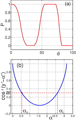
Fig. 2: (Color online) (a) The variation of the ratio P = S−/S with d. Here, S and S− represent, respectively, the area of the FR and the area of the gains corresponding to stable controls in this FR. The other parameters are the same as those in fig. 1. Periodically, P approaches 0 (1, respectively), which implies that every control with a gain in the FR is unstable (stable, respectively). (b) The intersection points α0,1 between the curve cos2[y*(α*) − α*] and the line A = aτ = 0.3 < 1.
Download figure:
Standard imageIn addition, since the FR rotates periodically around the origin which is located outside this FR, there exist infinitely many intervals of d, in which the FR has no interaction with the line n = 0. Thus, every n ≠ 0 in the FR implies an asymmetric gain matrix. Therefore, not a symmetric but an asymmetric gain matrix in front of the feedback control with time delay is vital for OS with particular frequencies. To find out such frequencies, we set ψ = 0, such that n = 0 and α = −dτ (mod π). Then, the NS conditions for local stability are not satisfied provided with α∈(α0,α1). Here, both α0 and α1 are the two solutions of the equation
as mentioned above and shown in fig. 2(b). Consequently, we get that

for  , that is,

are the intervals in which a symmetric gain matrix with any m is useless but an asymmetric one is essential for a successful OS.
Although model (1) has no persistent oscillation when a ⩽ 0, we still include the NS conditions for Cases II and III in table 1 since they are useful for realizing oscillation synchronization in complex systems later in this letter. Differently from A = aτ < 1 in Case I, there is no restriction on any finite time delay for these two cases. We also list the conditions for the limit situations of τ. Clearly, it is possible for Case III to guarantee the stability of model (2) when τ goes to +∞; nevertheless, it is impossible for the critical Case II.
Applications-oscillation death and synchronization
Now, we will validate the usefulness of the above-established NS conditions in coping with typical complex dynamical systems. First, we consider the FHNM [32, 33], which describes neuronal activity by the equations

The FHNM produces oscillations when the current input I is around I1, where I1 = (s + ζ)/δ + s3/3 − s is a supercritical Hopf bifurcation point at the equilibrium E(v0,w0) and s = (1 − δ )1/2. We aim to suppress these oscillations to E by a feedback control with time delay. We set

with ρ = (δ − v20 + 1)/2. Through the linear transformation

and by the linearization around E [31], the controlled FHNM can be transformed into equations of type (3), where the gain matrix is [m,−n;n,m]. In particular, a and d here can be regarded as functions of I for the FHNM (see fig. 3(a), and the gain matrix for the original controlled FHNM before the linear transformation reads

When n = 0, this gain matrix  becomes symmetric, i.e.,
  . By using the NS conditions of Case I in table 1, we conclude that for any m a symmetric gain matrix is useless to suppress the oscillation when τ = 0.1, ζ = 0.02, δ = 0.004, and = 200, and I∈(90,I1). However, we can find a particular unstable and asymmetric control with time delay to achieve OS for the FHNM. Both unsuccessful OS and successful OS are numerically depicted in figs. 3(b), (c), respectively.
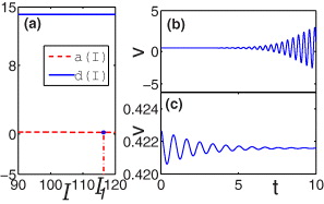
Fig. 3: (Color online) (a) The plots of functions a(I) and d(I) with respect to the argument I. Here, a(I) is slightly above 0 for I∈(90,I1). (b) An unsuccessful OS in the controlled FHNM by a stable and symmetric control (m = −4), and (c) a successful OS by an unstable and asymmetric control (m = 4 and n = −5).
Download figure:
Standard imageSecondly, we analyze the OD phenomenon which possibly occurs in a complex system of N identical dynamical units connected through time-delayed couplings [19]:

Here,  represents the state variable of each unit, {cij}N×N is a diagonalizable coupling matrix whose row sum
  is supposed to be m for all i = 1, ... ,N, and x0 = 0 is assumed as the equilibrium of each unit. It is easy to verify that the occurrence of OD can be determined by the stability of all the variational equations (VEs):

where λ1 = m is the eigenvalue of {cij}N×N associated to perturbations at x0 within the synchronization manifold (SM) and λ2,... ,N are the transversal eigenvalues [34]. For example, when each uncoupled unit satisfies model (1), q = 2 and the stability of the first VE is determined by the root distribution of eq. (4) as k = m and ψ = 0. According to the NS conditions established above for a symmetric control (ψ = 0) with time delay, despite A = aτ < 1, for any m the first VE is unstable and so OD cannot be observed physically when the oscillation frequency of the uncoupled unit is located in the intervals  as defined above. However, OD can be reached only when the frequency is not in
  , and the stability of the transversal VEs, in addition to the first VE, should be guaranteed through adjusting the eigenvalues λσ of {cij}N×N in light of the NS conditions. For some frequencies, the transversal eigenvalues might satisfy Re{λσ} > 0, which implies unstable control.
Finally and more significantly, we discuss periodic orbit synchronization in the above complex system. For a clear illustration, we suppose the uncoupled unit to be a three-dimensional system having a stable periodic orbit S(t) with period T. Thus, the Floquet exponents of S(t) become

where a < 0 [35]. We further set λ1 = m = 0, such that S(t) is within the SM. The other transversal VEs become

which, by virtue of the Floquet theory [35], can be further transformed into

if τ = pT and  [31]. We thus conclude that synchronization can be achieved if λ2,... ,N are adjusted to fulfill the NS conditions for Cases II and III in table 1. For example, one possible condition becomes

if all λ2... ,N are real and  with τ = pT.
Concluding remarks
Altogether, we have established NS conditions for OS through feedback control with time delays. We find that, when the time delay is appropriately selected, realization of OS crucially depends on the oscillation frequencies and the forms of control gains. Compared with the case of no time delay, an introduction of time delays brings an essential difference in the realization of OS.
Our results also suggest several directions for future research: i) the continuous dynamical model (1) could be replaced by some paradigmatic oscillating model in a discrete type; ii) our findings could be used in modulating the oscillations in real systems including preventing or generating the occurrence of OD and the synchronization phenomenon in the treatment of some mental diseases [8–12]; iii) the results could be used to analyze the dynamics of some higher-dimensional system which is controlled by the original time-delayed feedback controller, such as in systems biology (gene regulation) [7, 16, 26, 27]; iv) the deterministic control with time delays could be replaced by some stochastic control with or without time delays [36–38].
Acknowledgments
This work was supported by the NSF of China (Grant Nos. 10971035 and 61273014), and by Talents Programs (Nos. 10SG02, 11QH1400200 and NCET-11-0109).