


Abstract
Based on a phenomenological model with s± or s-wave pairing symmetry, the mixed-state effect on quasiparticle interference in iron-based superconductors is investigated by solving large-scale Bogoliubov-de Gennes equations based on the Chebyshev polynomial expansion. Taking into account the presence of magnetic field, our result for the s± pairing is in qualitative agreement with recent scanning tunneling microscopy experiment while for the s-wave pairing, the result is in apparent contradiction with experimental observations, thus excluding the s-wave pairing. Furthermore, we treat the effect of vortices rigorously instead of approximating the vortices as magnetic impurities, thus our results are robust and should be more capable of explaining the experimental data.
Export citation and abstract BibTeX RIS
Introduction
The discovery of iron-based superconductors [1] has triggered efforts to elucidate the superconducting (SC) pairing mechanism in these materials. One hotly debated issue is the symmetry and structure of the SC gap. Theoretically, it was initially suggested that the pairing may be established via spin fluctuations, leading to the so-called s± pairing symmetry ( defined in the 2Fe/cell Brillouin zone (BZ)). In this case the SC order parameter (OP) exhibits a sign reversal between the hole pockets (around the Γ point) and electron pockets (around the M point) [2–4]. Later, s-wave pairing symmetry without sign reversal was also proposed to be a possible candidate which is induced by orbital fluctuations due to the electron-phonon interaction [5]. Experimentally, the results about the pairing symmetry remain highly controversial as well. For example, in Ba0.6K0.4Fe2As2, an optimally hole-doped iron-based superconductor [6], the SC gaps measured by the angle-resolved photoemission spectroscopy (ARPES) can be approximately fitted by
  , with almost isotropic gaps on all the Fermi surfaces (FS) [7, 8], indicating the possible pairing symmetry to be either s± or s-wave. The situation is similar for optimally doped FeTe1−xSex with x ≈ 0.45 [9]. Neutron scattering experiments observed a resonance peak at
  below the SC transition temperature [10–13] as predicted by some theoretical works assuming s± symmetry [14, 15], thus at first glance they seemed to support each other. However, later theoretical works suggested that the experimentally observed resonance peak can also be reproduced by assuming s-wave pairing [16, 17].
Recently, in order to clarify the pairing symmetry, Hanaguri et al. used scanning tunneling microscopy (STM) to image the quasiparticle interference (QPI) patterns in the SC state [18]. They proposed that the relative sign of the SC OP can be determined from the magnetic-field dependence of quasiparticle scattering amplitudes and claimed that their experimental data were only consistent with the s± scenario but not the s-wave one. Soon after, the experimental results were put into question and argued instead to arise from the Bragg scattering but not due to the QPI because the observed peaks are too sharp [19]. On the other hand, the magnetic field will induce vortices into the system and lead to the inhomogeneity of the pairing OP in real space, thus affecting the QPI patterns. Theoretical analyzes performed previously have investigated the mixed-state effect on the QPI [20–22]. However, in ref. [20], only amplitude suppression of the OP near the vortex core was considered, without taking into account the phase variation. In ref. [21], the mixed-state effect was treated by using quasiclassical approximation and the QPI derived in this way was rather broad compared to the experimental observation. Furthermore, in ref. [22], only the effect of the Zeeman splitting was considered, which should be negligible with respect to the mixed-state effect. Thus there still lacks direct theoretical confirmation of the mixed-state effect on the QPI.
Therefore in this work we adopt a phenomenological model with s± pairing symmetry to study the influence of vortices on the QPI by directly solving large-scale Bogoliubov-de Gennes (BdG) equations in real space based on the Chebyshev polynomial expansion. For comparison, the problem is also studied for s-wave pairing. In this way the mixed-state effect on the QPI can be rigorously investigated and the results unambiguously support s± pairing symmetry in iron-based superconductors.
Method
We begin with an effective two-orbital model on a two-dimensional lattice [23], with a phenomenological form for the intraorbital pairing terms. The Hamiltonian can be written as
Here i and j are the site indices while α,β = 1,2 are the orbital ones. σ represents the spin and μ is the chemical potential. Then we consider potential scattering by nonmagnetic impurities through Vimp with iimp being the locations of the impurities.  is the intraorbital spin singlet bond OP, where Vij is the onsite (i = j) or next-nearest-neighbor (
 ) attraction which we choose to achieve the s-wave or s± pairing symmetry, respectively. Here we need to emphasize that the purpose of the present work is to study the mixed-state effect on the QPI by assuming s± or s-wave pairing symmetry, but not the mechanism of superconductivity in this type of compound. Thus we choose such an attractive interaction Vij only to reproduce the desired s± or s-wave pairing symmetry. Interestingly, based on this phenomenological model, the phase diagram [24] and vortex states [25] we derived are both in agreement with experimental observations, thus justifying the validity of the present approach. In the presence of a magnetic field B perpendicular to the plane, the hopping integral can be expressed as t'ij,αβ = tij,αβexp
 ![$[i\frac {\pi }{\Phi _{0}}\int _{j}^{i}\vect {A}(\vect {r})\cdot \mathrm {d}\vect {r}]$](https://content.cld.iop.org/journals/0295-5075/100/3/37002/revision1/epl14964ieqn6.gif) , where Φ0 = hc/2e is the SC flux quantum, and
, where Φ0 = hc/2e is the SC flux quantum, and  is the vector potential in the Landau gauge. The hopping integrals are

The Chebyshev polynomials can be written as ![$\phi _{k}(x)=\cos [k\arccos x]$](https://content.cld.iop.org/journals/0295-5075/100/3/37002/revision1/epl14964ieqn8.gif) and statisfy [26–29]
and statisfy [26–29]
where  , νk = π(1 + δk0)/2 and x∈[ − 1,1]. Next we define the Green's function matrix:

with C† = (··· ,c†j1↑,c†j2↑,··· ,cj1↓,cj2↓,··· ). Equation (1) can be diagonalized as

Here Q is a unitary matrix that satisfies (Q†MQ)rs = Drs = δrsEs and Φ = Q†C. The spectral function can be expressed as [26, 27]
Here r, s, γ = 1,··· ,L with L = 4NxNy and Nx (Ny) being the number of lattice sites along  (
( ) direction of the 2D lattice. a = (Emaxγ − Eminγ)/(2 −
  ) ( > 0 is a small number), b = (Emaxγ + Eminγ)/2,
  , ξγ = (Eγ − b)/a and
  .
.
If we further define the L-dimensional vectors e(o) and h(o) as e(o)γ = δγo and h(o)γ = δγo+2Ns (Ns = NxNy and o = 1,··· ,2Ns), we can express the self-consistent parameters as

where m = 2(jy + Nyjx) + β and n = 2(iy + Nyix) + α with ix,jx = 0,··· ,Nx − 1 and iy,jy = 0,··· ,Ny − 1.  ,
,  and
and  . N is the cutoff in the summation and gk is the kernel we convolute to avoid Gibbs oscillations [28]. In addition, f(x) is the Fermi distribution function. At zero temperature we have

Then we can solve the BdG equations self-consistently and the chemical potential is determined by the doping concentration. The calculation is repeated until the absolute error of the OP between two consecutive iteration steps and that of the total electron number are less than 10−4. The local density of states (LDOS) is given by
where  . Following ref. [18], we further define

and  is the Fourier transform of Zj(ω). Here
  is defined in the 1Fe/cell BZ in accordance with ref. [18].
The benefits of this method are threefold. First, it requires much less storage than the exact diagonalization method since the matrix M is sparse, thus we can solve large-scale BdG equations and obtain the QPI by Fourier transforming the real-space LDOS in sufficiently wide range. Second, it is applicable in parallel computation because the self-consistent parameters on each lattice site can be calculated separately. Third, the expansion scheme is very stable and efficient.
In our calculation, the magnitudes of the parameters are chosen as t1−4 = 1,0.4,−2,0.04. The FS in the 2Fe/cell BZ derived by using this set of parameters is shown in fig. 1. There are hole pockets around Γ and electron ones around M, thus the FS topology as well as the band structure we use can qualitatively represent iron-based superconductors. Furthermore, magnetic unit cells are introduced where each unit cell accommodates four SC flux quanta and the linear dimension is Nx × Ny = 80 × 80, corresponding to a magnetic field B ≈ 8.32 Tesla, close to the experimental value (10 Tesla) [18]. Vii and Vij ( ) are chosen to be −2.8 and −2, respectively. Moreover we introduce 12 randomly distributed impurities with Vimp = 0.3. The ratio of Nimpurity/Nvortex is chosen to be 3 in order to be consistent with the experimental observation (see fig. S2 in the supporting online material for ref. [18]). Emaxγ (Eminγ) is chosen as 1.5 (−1.5) band width. Throughout the paper, we set the system to be 20% hole-doped. In calculating the self-consistent parameters, we use the Jackson kernel

with = 0.001 and N = 500. For the LDOS we convolute the Lorentz kernel

with λ = 4, = 0.004 and N = λ/.
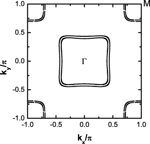
Fig. 1: The FS of our tight-binding model plotted in the 2Fe/cell BZ. The two pockets around Γ are hole pockets while those around M are electron ones.
Download figure:
Standard imageResults and discussion
First we consider the s± case. For Vimp = 0, fig. 2(a) shows that there exists a negative-energy in-gap peak in the LDOS at the vortex core center, in agreement with the experimental observation [30] and our previous results based on the exact diagonalization method [25], indicating the reliability of the Chebyshev polynomial-expansion scheme. Figure 2(c) plots the spatial distribution of Zj(ω), for B = 0 and at ω = Δ. The locations of the impurities can be clearly identified as the low-intensity spots. The corresponding  is shown in fig. 2(d). We notice that there are high-intensity peaks at
  ((±π,0) and (0,±π)) which arise from the interpocket scattering between the hole and electron pockets where the SC OP changes sign. Furthermore the intensities at
  ((±π,±π)) are much weaker than those at
  , consistent with the experimental observation [18]. This is because the intensity of the QPI is influenced by the relative sign of the SC OP between the two FS involved in the scattering process, through the coherence factor
  [18]. For iron-based superconductors,
  connects the electron pockets around (±π,0) and (0,±π), which preserves the sign of the SC OP if the paring symmetry is s±. In the case of weak scalar potential scattering as considered in the present work,
  is strongly suppressed for the
  that preserves the sign of the SC OP [31], leading to the lower intensity at
  than that at
  . On the other hand, along (±π,0) to (0,±π), there are broad high-intensity features. These should arise from the intrapocket scattering since the hole and electron pockets in our band structure are not circular, but more square-like. On the contrary, in ref. [27], these features do not show up, possibly due to the different band structure used. Upon applying the magnetic field, vortices are introduced into the system and their locations are denoted as the high-intensity spots in fig. 2(e). We notice that the vortices form a triangular lattice and none of them is pinned by the impurities since the impurity density is dilute and its strength is weak. In this work, the arrangement of the vortices as well as the position of the vortex cores are completely determined by the self-consistent calculation, and we did not assume any form of the vortex lattice. That is, we have tried various initial values and the converged results always led to the triangular vortex lattice as shown in fig. 2(e) (with or without the impurities). This means that the triangular vortex lattice is a stable state of the system. In all the calculations, the square vortex lattice as made in ref. [27] or other forms never appear as the converged results, thus they are energetically unfavorable for iron-based superconductors. Experimentally, the triangular vortex lattice has been observed in Ba0.6K0.4Fe2As2 (see fig. 5 in ref. [30]). In addition, in LiFeAs the vortices form quasihexagonal lattice at low field and become disordered at higher field. Nevertheless, they are never arranged into a square lattice [32]. Therefore in the present work, since we can only get the triangular vortex lattice self-consistently and the experiments did not observe the square vortex lattice in iron-based superconductors, we concentrate on the triangular one and do not consider other forms. In this case, from fig. 2(f) we can see that there exist additional peaks at
  , whose intensities are enhanced by the application of the magnetic field and they are due to the interpocket scattering between different electron pockets (see fig. 1 in ref. [18]). Figure 2(b) shows the magnetic-field–induced change in the QPI intensities defined as
  . In the presence of the time-reversal symmetry breaking due to the magnetic field, the phase of the SC OP precesses by 2π about each vortex and its amplitude vanishes at the vortex core center. Both the phase variation and the inhomogeneity in the amplitude can scatter quasiparticles. While the former produces Doppler-shift scattering [33] that is odd under time reversal with
  being like that of magnetic impurities, the latter causes inhomogeneous Andreev scattering. Both of the scattering will enhance (suppress) the QPI intensities at those
  points that preserve (reverse) the sign of the SC OP [31]. Thus the sign-preserving scatterings at
  (
( connects the FS with the same sign of the SC OP) are enhanced while the sign-reversing scatterings at
  (
( connects the FS with the opposite sign of the SC OP) are suppressed. These phenomena are most pronounced around ω ≈ Δ. Away from it, the intensity at
  diminishes, since
  connects the hole and electron bands with different dispersion. On the other hand, spotty features remain at
  even at low and high energies, which may be ascribed to a field-induced Bragg (-like) component [18]. Both the locations and the sharpness of the QPI peaks shown in figs. 2(b), (d) and (f) are in reasonable agreement with the experimental data [18], suggesting that the experimentally observed peaks are indeed due to the QPI but not the Bragg scattering as argued in ref. [19].
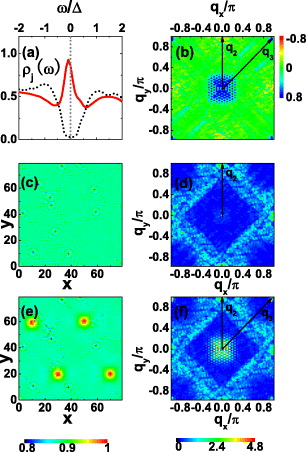
Fig. 2: (Colour on-line) For s± pairing symmetry. (a) The LDOS at the vortex core center (red solid line) and at B = 0 (black dotted line) as a function of the reduced energy ω/Δ. Here 2Δ is the SC gap between two SC coherence peaks in the LDOS at B = 0. The gray-dotted line indicates the position of ω = 0. (b)  at ω = Δ. (c) and (d) show Zj(ω = Δ) and
  at B = 0, respectively. (e) and (f) are the same as (c) and (d), respectively, but for B ≠ 0. (c) and (e) share the same colour scale while the case is similar for (d) and (f).
Download figure:
Standard imageNext we consider the s-wave case. For Vimp = 0, the LDOS at B = 0 (black dotted line) and at the vortex core center (red solid line) shown in fig. 3(a) are also consistent with those obtained by exact diagonalization [34], again suggesting the validity of the current polynomial-expansion scheme. From fig. 3(c) we notice, the QPI in the presence of impurities at B = 0 exhibits no pronounced peaks at either  or
or  , as compared to the clear peaks at
  in the s± case as shown in fig. 2(d). This is because for s-wave pairing,
  also connects the FS with the same sign of the SC OP, thus the QPI intensity at this wave vector is suppressed for potential scattering as compared to the s± case. After applying the magnetic field, the intensities at
  are enhanced and they form sharp peaks as shown in fig. 3(d), similar to the s± case. At last, from the magnetic-field–induced change in the QPI intensities plotted in fig. 3(b) we can see, the intensities are enhanced at
  but remain almost unchanged at
  . The lack of distinct structures at
  is in stark contrast to the s± case and is inconsistent with the experimental observations [18]. Therefore, the different behaviour of the QPI intensities at
  in the s± and s-wave pairing cases makes it possible to distinguish these two types of pairing symmetry since the STM experiment observed clear structures at
  , thus excluding the possibility of s-wave pairing in iron-based superconductors.
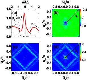
Fig. 3: (Colour on-line) For s-wave pairing symmetry. Panels (a), (b), (c) and (d) are similar to figs. 2(a), 2(b), 2(d) and 2(f), respectively. Panels (c) and (d) share the same colour scale.
Download figure:
Standard imageSummary
In summary, by using the Chebyshev polynomial expansion to directly solve large-scale BdG equations in real space, we have investigated the mixed-state effect on QPI in iron-based superconductors by assuming s± or s-wave pairing symmetry. For the s± pairing, the QPI intensities at  which connects the FS with the opposite sign of the SC OP are suppressed by the application of the magnetic field while the situation at
  is reversed where
  connects the FS with the same sign of the SC OP. The obtained results at both B = 0 and B ≠ 0 are in qualitative agreement with experiment, suggesting that the experimentally observed peaks are indeed due to QPI. On the other hand, for the s-wave pairing, the QPI intensities at
  are featureless both with and without the magnetic field. Based on the available experimental data, the s-wave pairing can be excluded in iron-based superconductors.
In addition, we want to take this opportunity to compare our work with the previous ones which also studied the QPI in iron-based superconductors by using different band structures or methods. For s± paring, without the magnetic field, our results are similar to those in refs. [20, 22, 35, 36] where strong QPI peaks appear at  (see fig. 4 in refs. [20, 35, 36] and fig. 2 in ref. [22]). With the magnetic field, the QPI patterns in refs. [20–22, 35, 36] all lack clear peaks at
  (see fig. 4 in refs. [20, 36], fig. 8 in ref. [21], fig. 2 in ref. [22] and fig. 5 in ref. [35]). On the contrary, since we take both the phase variation and amplitude suppression induced by vortices into account, thus less approximation of the physics in involved in our calculation, we can get sharp QPI peaks at
  in agreement with experiment.
Furthermore we need to point out that although the method used in the present work is similar to that in ref. [27], the model and results are completely different. Our model is a multi-orbital one as compared to the single-orbital one adopted in ref. [27]. Thus the FS topology is drastically different between this two models (see fig. 1 and fig. 4 in ref. [27]). Besides, we assumed s± or s-wave pairing symmetry in the present work while the authors in ref. [27] considered d-wave pairing symmetry. Since the QPI is closely related to the FS topology and the SC pairing symmetry, thus the QPI patterns derived in our work and those in ref. [27] share no similarity and cannot be compared to each other. Most importantly, in ref. [27] the authors concluded that only pinned vortex can lead to the correct QPI patterns. However in our work, the vortices are not pinned by any impurities and we can still get the QPI patterns in qualitative agreement with the experimental observations. This is consistent with the experimental conclusion that no appreciable correlation is observed between the location of vortices and the magnitude of field-induced change in the QPI intensity (see the supporting online material for ref. [18]), suggesting different scattering mechanism in iron-based superconductors and that studied in ref. [27].
Acknowledgments
This work was supported by NSFC (Grants No. 11204138 and No. 11175087), Natural Science Foundation of Jiangsu Province, China (Grant No. BK2012450), Natural Science Foundation of the Higher Education Institution of Jiangsu Province, China (Grant No. 12KJB140009), National Key Projects for Basic Research of China (Grant No. 2009CB929501), and by China Postdoctoral Science Foundation (Grant No. 2012M511297). PQT acknowledges the hospitality of ICTP.
In this work, firstly, the system is set to be 20% hole-doped. At this doping level, the FS topology derived from our band structure contains both the hole pockets around the Γ point and the electron ones around the M point with the hole and electron pockets being quasinested by the wave vector  . Secondly, we have assumed that the pairing symmetry is s± or s-wave like. In this case, based on such a FS topology, there are no nodes on all the FS and the gaps are almost isotropic on each FS. Thirdly, we did not consider the spin-density-wave (SDW) order in our system. Thus our work applies to those iron-based superconductors such as the optimally doped Ba1−xKxFe2As2, BaFe2−x(Co, Ni)xAs2 and FeTe1−xSex, where the FS topology, the nonexistence of nodes and the almost isotropic gaps measured by ARPES experiments [7–9, 37] as well as the disappearance of SDW observed by neutron scattering experiments [10–13] are in agreement with our work. The exact doping is not important here as long as the hole and electron pockets can be quasinested by
  , since the QPI studied in this work and probed by STM experiments is sensitive to the phase difference between two
  on different FS connected by
  . Our work cannot be applied to the recently discovered KxFe2−ySe2 compounds because the FS topology in this system contains only the electron pockets [38] and is qualitatively different from the above-mentioned compounds. Furthermore, those iron-based superconductors with possible nodes on the FS, such as LaFePO [39] and Ba(FeAs1−xPx)2 [40], are not considered in our work. The study of QPI in these systems as well as the parent compounds [41] will constitute our future investigation.