
Abstract
The objective of quantitative photoacoustic tomography (qPAT) is to reconstruct the diffusion, absorption and Grüneisen thermodynamic coefficients of heterogeneous media from knowledge of the interior absorbed radiation. It has been shown in Bal and Ren (2011 Inverse Problems 27 075003), based on diffusion theory, that with data acquired at one given wavelength, all three coefficients cannot be reconstructed uniquely. In this work, we study the multi-spectral qPAT problem and show that when multiple wavelength data are available, all coefficients can be reconstructed simultaneously under minor prior assumptions. Moreover, the reconstructions are shown to be very stable. We present some numerical simulations that support the theoretical results.
Export citation and abstract BibTeX RIS
1. Introduction
In photoacoustic tomography (PAT), near infrared (NIR) light propagates into a medium of interest. As a fraction of the incoming light energy is absorbed, the medium heats up. This results in mechanical expansion and the generation of compressive (acoustic) waves. The acoustic waves propagate to the boundary of the medium where they are measured. From knowledge of these (time-dependent) acoustic measurements, one attempts to reconstruct the diffusion, absorption and Grüneisen thermodynamic properties of the medium of interest [2, 7, 19, 31, 33, 36, 39, 47, 55–57].
The reconstruction problem in PAT is a two-step process. In the first step, one reconstructs the absorbed energy map (multiplied by a coefficient), H defined in (2) below, from the measured acoustic signals on the surface of the medium. This is a relatively well-known inverse source problem for the wave equation that has been extensively studied in the past [1, 16, 21, 22, 25–28, 32, 34, 37, 39, 40, 50–53]. In the second step, often called quantitative PAT (qPAT), the objective is to reconstruct the diffusion coefficient D in (1), the absorption coefficient σ in (1) and the Grüneisen coefficient Γ in (2), from the reconstructed energy data H. This step has recently attracted significant attention from both mathematical [3, 4, 8–10] and computational [11, 17, 18, 20, 24, 23, 35, 45, 46, 59, 61] perspectives. Mathematically, the reconstruction problem in this step is very similar to the diffuse optical tomography (DOT) problem except that in DOT we have boundary current data, while here in qPAT we have interior absorbed energy data. The use of interior data improves the stability, and thus the resolution, of the reconstruction significantly. This is the main advantage of PAT over DOT.
Most of the studies in the past have assumed that the Grüneisen coefficient is a constant and is known so that only the absorption and diffusion coefficients are to be reconstructed. As recently pointed out in [17, 19, 48], it is more realistic to consider Γ as a function of space. In this work, we treat Γ also as an unknown. We thus aim at both Γ and the optical coefficients. Note that unlike the reconstruction of the absorption coefficient σ and the diffusion coefficient D, the reconstruction of Γ is a linear inverse problem since the data H we have are linearly proportional to Γ. This means that if both σ and D are known, then we can simply solve the diffusion equation (1) and compute the energy E = σu. Then Γ is reconstructed as Γ = H/E.
The work in [9] has shown that with data at only one wavelength, the reconstruction of the three coefficients simultaneously is not unique. In fact, only two of the three coefficients can be reconstructed without other a priori information. The objective of this work is exactly to reconstruct all three coefficients by using measured data of different wavelengths and a priori information on the form of the coefficients. We show that the reconstruction can be done when the coefficients take specific forms. One specific case of practical importance is that if the dependence of the coefficient on the spatial variable and on the wavelength variable can be separated, then they can be reconstructed with spectral data stably.
The paper is structured as follows. In section 2, we reformulate the inverse problem of quantitative PAT in the setting of multiple wavelength illuminations and present uniqueness and stability theory regarding the inverse problem in simplified settings. We then present in section 3 numerical procedures to reconstruct the unknown coefficients. We present some numerical simulation results with synthetic data in section 4. Conclusions and further remarks are offered in section 5.
2. Uniqueness and stability results
Let us denote by X a bounded domain in  (d = 2, 3) with the smooth boundary ∂X, and
  the set of wavelengths at which the interior data are constructed. In the diffusive regime, the density of photons at the wavelength λ,
  solves the following diffusion equation:

where  and
and  are the wavelength-dependent diffusion and absorption coefficients, respectively, and
  is the illumination pattern in photoacoustic experiments. The wavelength-dependent interior data constructed from the inversion of the acoustic problem are given by

where  is the non-dimensional Grüneisen coefficient that relates the absorbed optical energy σu to the increase in pressure H. The thermodynamic coefficient Γ measures the photoacoustic efficiency of the medium.
The problem of multi-spectral qPAT is to reconstruct the coefficients  ,
,  and
and  from interior data of the form (2). The results in [9] state that without further a priori information, we cannot uniquely reconstruct all three coefficients. In fact, only two quantities related to the three coefficients, i.e. the functionals
  and
and  defined in (5) below can be reconstructed. The objective of this work is to show that when data of multiple wavelengths are available, we can recover the uniqueness in the reconstructions with relatively little additional a priori information. To obtain results that are as general as possible, we allow the diffusion and absorption coefficients to be arbitrary functions of the wavelength and assume that the Grüneisen coefficient can be written as the product of a function of space and a function of wavelength. More precisely, the coefficients take the following form:

where γ(λ) is a function assumed to be known. This assumption is not sufficient to guarantee unique reconstructions. We need to assume a little more on the coefficients. Our main assumption is as follows.
- (A1)There exist two known wavelengths λ1, λ2 ∈ Λ so that
 for some known positive constant ρ, while for all .This assumption essentially requires that the dependence of the diffusion and absorption coefficients is different for at least two wavelengths. Otherwise, we would simply be able to eliminate the spectral dependence from equation (1). We will see later on that this assumption is satisfied by most coefficient models employed by researchers in the community. We also need some assumptions on the regularity and boundary values of the coefficients. We assume, denoting by the space of p-times differentiable functions in X, that
 - (A2)the function, and its boundary value D|∂X is known. The functions .


We now present the main uniqueness result on reconstructions with multi-spectral data.
Theorem 2.1. Let (D, σ, Γ) and  be two sets of coefficients given in (3), with γ(λ) known, satisfying assumptions (A1) and (A2). Then there exists an open set of illuminations
  such that the equality of the data

in X × Λ implies that

in X × Λ provided that the values of the diffusion coefficient agree on the boundary:  for all λ ∈ Λ.
Proof. With the regularity assumptions on the diffusion coefficient, we can recast equation (1), using the Liouville transform  , as
, as

with the interior data H(x, λ) = v(x, λ)/χ(x, λ), where χ and q are defined respectively as

Let us denote by  and
and  the solutions of (4) with the illuminations
  and
and  respectively. Then it is straightforward to check that [9]
Since  is known, this is a transport equation for
  with the vector field
  . By the results of [9], there exist the well-chosen illuminations g1 and g2 (and thus
  and
and  ) such that the vector field is smooth enough with the positive modulus
  . This ensures that the transport equation is uniquely solvable for v21. Once v21 is reconstructed, we can reconstruct χ = v1/H1 and then q = −Δv1/v1.
Now let λ1, λ2 ∈ Λ be two wavelengths as in assumption (A1). We first reconstruct the two pairs of functionals ( ) and (
 ). With the assumption that
  , we obtain after some algebra using the above equations that

where the function  is defined as

Using the conditions in assumptions (A1) and (A2), the denominator in Q does not vanish and Q is bounded. The elliptic equation (7) can then be solved uniquely as shown in [9] to reconstruct  . We then find


Once  is reconstructed, then so is
  . The results in [9, corollary 2.3] then allow us to reconstruct
  and
and  for all λ ∈ Λ.
It has been shown in [9] that the reconstruction of v1 (and thus that of χ and q as well) is Lipschitz stable for each fixed wavelength. Because the solution of (7) is stable with respect to Q, we deduce that the reconstruction of the  (and thus
  ) is stable. Precise stability estimates similar to those in [9, theorem 2.4] can be derived.
The coefficient model (3) is quite general and covers many of the models used in the literature. For instance, we may consider the following standard model [13–15, 17, 19, 29, 35, 41, 42, 48, 49, 54, 58, 60]:
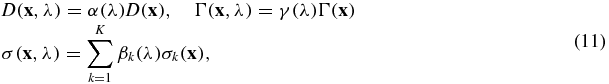
where the functions α(λ), {βk(λ)}Kk = 1 and γ(λ) are assumed to be known. In other words, all three-coefficient functions can be written as products of functions of different variables. Moreover, the absorption coefficient contains multiple components. This is the parameter model proposed in [17, 19, 29, 35, 42, 49] to reconstruct chromophore/fluorochrome concentrations from optical measurements. The following result regarding model (11) is a natural extension of theorem 2.1.
Corollary 2.2. Let  ,
,  and
and  be as in (11) and satisfying assumptions (A1) and (A2). Assume further that there exist K wavelengths such that the matrix B with elements Bkj = βk(λj) (1 ⩽ k, j ⩽ K) is non-singular. Then the coefficients
can be uniquely reconstructed from the well-chosen data  ,
,  .
.
Proof. Theorem 2.1 allows the unique reconstruction of  ,
,  and
and  . Since B is non-singular, we can invert the linear system
  , j = 1, ..., K, to recover
  .
.
3. Reconstruction methods
We now present two numerical reconstruction methods for the multi-spectral qPAT problem.
3.1. The vector field method
The first method is based on the constructive uniqueness proof in the previous section. The proof provides an explicit procedure to reconstruct the unknown coefficients. The main step is to solve the transport equation (6) for v21. Let us denote by {λj}Kj = 1 the wavelengths at which data are measured. For a general pair of coefficients of the form (3) that satisfy assumptions (A1) and (A2), the algorithm proceeds as follows.
The vector field algorithm
- Step 2. Construct and as
- Step 5. Recover from .
- Step 6. Solve for by repeating the following steps for 3 ⩽ j ⩽ K.
- Step 6(a). Solve the transport equation (6) for.
- Step 6(b). Solve the following elliptic equation for:
- Step 6(c). Reconstruct and .


Step 6 is the main algorithm that we used in [9] for solving the mono-spectral qPAT problem for the case when  is known. Equation (13) is obtained by rewriting the diffusion equation (1) for u1 using the fact that Du21 = v12. As long as g1 ⩾ c0 > 0 everywhere on the boundary, this elliptic problem is well-posed for 1/u1. For more details on the vector field method in the mono-spectral case, including the discussion on dealing with noisy data, we refer to [9].
The same algorithm can be used when the simplified coefficient model (11) is considered. In that case, step 6(b) is not needed anymore. This is because once  and
and  in (11) are reconstructed,
  (1 ⩽ j ⩽ K) can be reconstructed from the solution
  to the transport equation.
The uniqueness results we presented hold only for coefficients that are regular enough, satisfying the regularity assumptions in (A2). So is this vector field algorithm that we just described. In practice, we do not know a priori whether or not the coefficients to be reconstructed satisfy this assumption. We thus have to make sure that  is smooth enough so that we can take the second-order derivatives without problem. That is the reason we added a smoothing process to v in step 2 of the algorithm. The kernel
  of the convolution operator
  is a smooth function. Here we take
  to be a Gaussian whose variance is used to control the strength of the smoothing. The strength of the smoothing is determined by looking at the image of
  . The smoothing, however, does not cause many problems for the solution of the next elliptic problem as we know that the solution of the elliptic problem is stable with respect to changes in Q.
3.2. The nonlinear least-squares method
The second approach to solve numerically the inverse problem is to reformulate the reconstruction problem as a data-driven minimization problem. More precisely, we look for the coefficients in the form of (3) that minimize the following mismatch functional:

where N ⩾ 2 is the number of different spatial source patterns used for a fixed wavelength. In the theoretical results we presented in section 2, N = 2. The data predicted by the model are denoted as  , with
  being the solution of the diffusion equation (1) with the ith source pattern
  . The real interior data, that is, the data constructed from acoustic measurement, are denoted by
  .
.
We solve the minimization problem by a quasi-Newton method with the BFGS updating rule on the Hessian operator [12, 30, 38, 44]. This method requires the Fréchet derivatives of the functional Φ with respect to the unknowns D, σ and Γ. These derivatives can be computed in the following way. Let us denote by  the solution of the adjoint problem

with  . Then it is standard to show that
Theorem 3.1. The nonlinear least-squares functional ![$\Phi : [L^2(X\times \Lambda )]^3 \mapsto \mathbb R$](https://content.cld.iop.org/journals/0266-5611/28/2/025010/revision1/ip407887ieqn85.gif) is Fréchet differentiable with respect to D, σ and Γ. The Fréchet derivatives are given respectively by
is Fréchet differentiable with respect to D, σ and Γ. The Fréchet derivatives are given respectively by


where  denotes the usual inner product in L2(X × Λ).
When model (11) is employed, the derivatives with respect to σ have to be replaced by the derivatives with respect to each σk (1 ⩽ k ⩽ K). These derivatives can be simply computed by using (18) and the chain rule. More precisely,

Compared with the vector field method in the previous section, the nonlinear least-squares method is a very general method. However, it is computationally more expensive. In each quasi-Newton iteration, we need to solve several forward and adjoint problems to evaluate the value of the objective function and the Fréchet derivatives. The method is thus slow. However, since the diffusion equation (1) and its adjoint (15) are elliptic problems that can be solved efficiently with finite-element methods, the overall reconstruction cost is reasonably low.
4. Numerical simulations
We now present some numerical simulations using synthetic data to support the theory that is developed in the previous section. To simplify the presentation, we consider only two-dimensional problems, even though the uniqueness results and the reconstruction methods hold in three-dimensional domains as well. The domain we consider is the square: X = (0, 2 cm) × (0, 2 cm). Material properties of the medium will be provided in specific cases.
In the first set of numerical experiments, we show reconstruction results for smooth coefficients. The coefficients take the forms given in (11) with two components in the absorption coefficient, i.e. K = 2. The spectral components of the coefficients are given as follows:

where the normalization wavelength λ0 is included to control the amplitude of coefficients. These weight functions are by no means what they should exactly be in practical applications. However, the specific forms do not have impacts on the results of the reconstruction. The spatial components of the coefficients are given as

Four illuminations are used, two at each wavelength. The reconstruction results with clean data, i.e. synthetic data without being polluted by additional random noise, are shown in the second row of figure 1. Note that the data used in this case indeed contain noise that comes from the discretization of the continuous PDE model, which is very small since we used a very fine discretization. The reconstructions are almost perfect, with overall quality very similar to those presented in mono-spectral data [9], as can be seen from the plots and the cross-sections (red dashed) in figure 2. The third row of figure 1 presents one typical realization of reconstruction results with data containing 5% extra additive random noise. The cross-sections of the reconstruction along the line y = 1 are shown in figure 2 (blue dashed). The results are still very accurate, with overall quality comparable to those results obtained in [9].
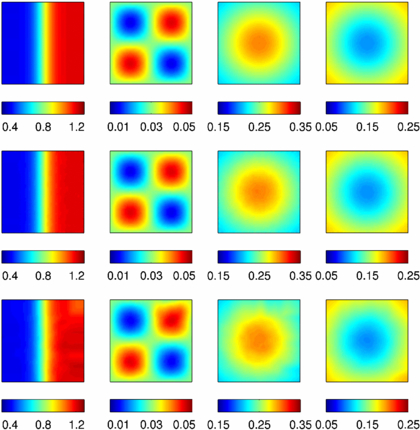
Figure 1. The reconstructions of the coefficients ( ,
,  ,
,  ,
,  ). From top to bottom: true coefficients, reconstructions with clean data and reconstructions with data containing 5% random noise.
Download figure:
Standard image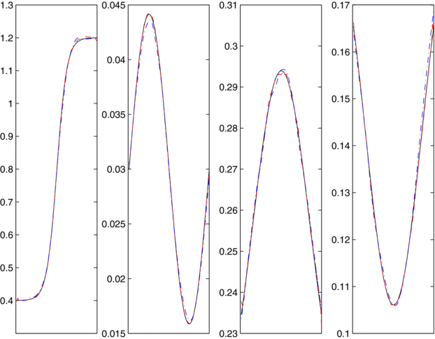
Figure 2. Cross-sections of plots in figure 1 along the axis y = 0.75. Shown are true coefficients (solid line), reconstruction with noise-free data (red dashed) and reconstructions with noisy data (blue dashed).
Download figure:
Standard imageIn the second set of numerical experiments, we show reconstruction results for piecewise constant coefficients with the numerical minimization algorithm that we introduced in the previous section. The true coefficients are shown in the first row of figure 3. We again use four illuminations of two different wavelengths. The reconstructions with clean and noisy data are presented on the second and third rows of figure 3, respectively. In the case of noisy data, we regularized the nonlinear least-squares problem with the Tikhonov regularization term  . The strength ρ of the regularization is taken after a few tests with different values. The effect of the regularization is mainly to smooth out the additive noise in the data. It also smooths out part of the jumps across the interfaces of coefficient discontinuities, as can be seen from the plots in the third row of figure 3. To better visualize the quality of the reconstructions, we again plot the cross-sections of the reconstructed coefficients in figure 4. We observe that discontinuous coefficients can be reconstructed as accurately as smooth coefficients, even though the discontinuity is smeared out in the former case.

Figure 3. The reconstructions of piecewise constant coefficients ( ,
,  ,
,  ,
,  ). From top to bottom: true coefficients, reconstructions with clean data and reconstructions with data containing 5% random noise.
Download figure:
Standard image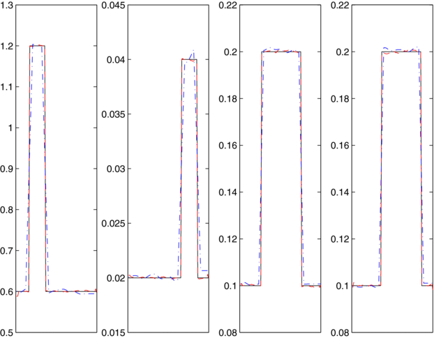
Figure 4. Cross-sections of true coefficients (solid line) and the reconstructed coefficients with noise-free data (red dashed) and a typical realization of noisy data (blue dashed) in figure 3 along the axis y = 1.0.
Download figure:
Standard image5. Concluding remarks
We presented in this paper some theoretical results for quantitative photoacoustic tomography with multi-spectral interior data to reconstruct the Grüneisen, absorption and diffusion coefficients simultaneously. We showed the uniqueness of the solution to the inverse problem under minor assumptions on the form of the coefficients. One specific case of practical importance is that, if the dependence of the coefficient on the spatial variable and on the wavelength variable can be separated, the spatial components of all three coefficients can be reconstructed with spectral data uniquely and stably.
We presented a vector field-based algorithm and a general nonlinear least-squares-based method for the numerical reconstruction of smooth and rough coefficients. We showed by numerical simulations that the reconstructions are very accurate for both types of coefficients, assuming that the interior data H constructed from measured acoustic data are accurate enough. The reconstructions are stable with Lipschitz type stability estimates that are identical to those in [9].
The uniqueness results that we obtained in this paper depend on the illuminations that are selected. In other words, uniqueness only holds when appropriate illuminations are used. Fortunately, the characterization of these 'well-selected' illuminations is identical to that presented in [9]. In fact, as pointed out in [9], many illumination pairs that we have used work, in the sense that they generate the data H1 and H2 such that the condition  holds, and thus the transport equation (6) is uniquely and stably solvable.
The results of this paper and [9] are all based on diffusion theory for light propagation in tissues. It is well known that the phase-space radiative transport model [5, 6, 43] is a more accurate light propagation model for this application. Uniqueness and stability results for the transport model have been developed in [8] in the situation where measurements from all possible illuminations are available. Numerical simulations have also been reported [20]. It would be interesting to extend the study in [8] to include an unknown variable Grüneisen coefficient.
Acknowledgments
We would like to thank Professor Simon Arridge (University College London) for useful discussion on the simplified coefficient model (11) in optical and photoacoustic tomography. KR was supported in part by NSF grant DMS-0914825. GB was supported in part by NSF grants DMS-0554097 and DMS-0804696.