


Abstract
Based on the accurate color excess  of more than 4 million stars and the
  of more than 1 million stars from Sun et al., the distance and extinction of the molecular clouds (MCs) in the Magnani–Blitz–Mundy catalog at ∣b∣ > 20° are studied in combination with the distance measurement of Gaia/EDR3. The distance, as well as the color excess, is determined for 66 MCs. The color excess ratio
  is derived for 39 of them, which is obviously larger and implies more small particles at smaller extinction. In addition, the scale height of the dust disk is found to be about 100 pc and becomes large at the anticenter direction due to the disk flaring.
Export citation and abstract BibTeX RIS

Original content from this work may be used under the terms of the Creative Commons Attribution 4.0 licence. Any further distribution of this work must maintain attribution to the author(s) and the title of the work, journal citation and DOI.
1. Introduction
The study of molecular clouds (MCs), the site of star formation (Blitz & Williams 1999), is important for the information on the initial mass function of stars and the buildup of galaxies. Molecular clouds in the Milky Way are the nearest and most accessible star-forming sites. Carbon monoxide is the main tracer of MCs, which is much more easily excited and observed than H2 and is used to detect a large number of MCs in many large-scale joint observations of the galaxy (e.g., Magnani et al. 1985; May et al. 1997; Dame et al. 2001). However, the distance as the fundamental and key parameter for studying MCs is often difficult to determine. Many distance measurement methods, such as stellar photometric parallax and period–luminosity relation, are not suitable for MCs.
Previously, a popular method was to estimate the distance to the clouds using Galactic kinematics, i.e., the distance at which the radial velocity of the cloud corresponds to the rotation curve of the Galactic disk (e.g., Brand et al. 1994; May et al. 1997; Nakagawa et al. 2005; Roman-Duval et al. 2009; García et al. 2014; Miville-Deschênes et al. 2017). This technique is widely applied to estimate the distances to a large number of MCs in the inner disk of the Galaxy (e.g., Roman-Duval et al. 2009). But the well-known problems are the large uncertainty induced by the presence of peculiar and noncircular motions and the ambiguity where one velocity can correspond to two distances at either side of the tangent point. Another frequently used method is to find the distance to the objects associated with a cloud and to place the cloud at the same distance; for instance, many clouds have produced young OB associations of stars for which distances can be estimated. This method can be applied to some specific cases.
Both of the above methods are applicable only to low-latitude clouds in the disk because high-latitude clouds deviate a lot from the disk rotation curve and have no young massive stars. Because MCs possess not only high-density gas but also high-density dust, their extinction significantly exceeds the surrounding diffuse interstellar medium. Thus, the distance to MCs can be inferred from the high extinction they cause (Goodman et al. 2009; Chen et al. 2017). Early in 1923, Wolf (1923) first effectively described Wolf diagrams based on star counts in obscured versus reference fields to determine the distance to MCs, and Magnani & de Vries (1986) applied the Wolf diagrams to a small subset of Magnani–Blitz–Mundy (MBM) clouds. Using the two-dimensional (2D) Galactic extinction maps, Dobashi (2011) identified more than 7000 MCs based on the idea that high extinction is caused by MCs. As the extinction map is 2D, no distance information can be obtained. With the 3D extinction maps, which are constructed by comparing the observed color distributions of Galactic giant stars with those predicted by the Galactic model, Marshall et al. (2009) cataloged over 1000 clouds together with their distance information and determined that the errors of their distances are about 0.5–1 kpc. Comparing the stars in front of the clouds, which have little extinction, with the predictions of the Galactic model, Lada et al. (2009) and Lombardi et al. (2011) estimated the distances to many clouds. With the multiband photometry by Pan-STARRS1 (Kaiser et al. 2010) and the resultant color indexes of numerous stars, Schlafly et al. (2014) derived the distances to 18 well-known star-forming regions and 108 MCs at high Galactic latitude selected from Magnani et al. (1985) and Dame et al. (2001) according to the breakpoint of the extinction.
The distances obtained in these studies are not measured directly but with the help of some stellar or Galactic model and suffer relatively large uncertainty. The Gaia mission has changed this situation drastically. The Gaia/DR2 catalog (Gaia/DR2; Gaia Collaboration et al. 2018) provides the distances to more than a billion stars, renewing the way to determine the distance to MCs by their extinction. With the Gaia/DR2 data, Zucker et al. (2019) present a uniform catalog of accurate distances to local MCs according to the breakpoint of the extinction. Yan et al. (2019) obtain the distances to MCs at high Galactic latitudes (∣b∣ > 10°) from the parallax (Lindegren et al. 2018) and G-band extinction (AG ) measurements of the stars at the cloud's sight line from Gaia/DR2. Based on the 3D dust reddening map and estimates of color excesses and distances of over 32 million stars, Chen et al. (2020) identified 567 dust/MCs within 4 kpc from the Sun at low Galactic latitudes (∣b∣ ≤ 10°) with a hierarchical structure identification method and obtained their distance estimates by a dust model-fitting algorithm. Benefiting from the large number of stars for the individual MCs and the robust estimates of the stellar distances from Gaia/DR2, the errors of the distances in these works are typically only about 5%.
The high-latitude MCs are generally optically thin, which leads to much smaller extinction than those in the disk, and usually very close, thus a precise measurement of extinction and distance to the stars is necessary to estimate their distance by the extinction method. Spectroscopy can be used to determine the stellar intrinsic color index and thus extinction is usually more accurate than multiband photometry. The general inefficiency of spectroscopy in comparison with photometry has recently been compensated by large-area multiobject spectroscopy such as the LAMOST survey, which has observed almost 10 million stars. Using the stellar parameters derived from the LAMOST and GALAH surveys, we (Sun et al. 2021, Paper I hereafter) determined the color excess  accurate to ∼0.01 mag on average toward about 4 million stars. In addition, the color excess
  is calculated for more than 1 million stars accurate to ∼0.1 mag. Moreover, Gaia/EDR3 was recently released with apparently more precise measurements of stellar parallaxes and distances. The combination of the accurate color excess and distance brings about the possibility of determining the distances to the MCs at high latitude. In addition, the dust property in the high-latitude clouds may be inferred from the color excess ratio of
  . Welty & Fowler (1992) studied the low-resolution UV spectra of the B3 V star HD 210121 located behind the high-latitude MC DBB 80 and obtained an extinction curve with a very steep rise in the far-UV. The extremely steep far-UV extinction and the augmentation of the intensity at 12 μm are consistent with the presence of an enhanced population of very small grains. We (Paper I) also find that there may be more small dust grains at high than at low galactic latitude, which is supported by the steeper increase of extinction toward the FUV band.
This paper is part of an ongoing project to study the extinction and dust as well as the 3D distribution of MCs at high latitude based on the spectroscopic and astrometric measurements of stars. This work focuses on the MBM high-latitude MCs.
2. Sample and Data
Blitz et al. (1984) started a project to conduct a systematic search of high-latitude MCs using the CO line observation of potentially obscured regions identified from the Palomar Observatory Sky Survey prints, which was followed up and completed by Magnani et al. (1985) (MBM) 3 . This project resulted in 124 detections of MCs with ∣b∣ > 20°. We adopt the center positions of the MCs from MBM, and the size as well if given. For the 88 MCs whose size is unavailable in MBM, a radius of 90' is taken as default, which is approximately the average size of the high-latitude MCs (Dutra & Bica 2002).
The tracers for the extinction and distance of high-latitude clouds are chosen from Paper I. Using the blue-edge method (see Jian et al. 2017 and Sun et al. 2018), Paper I calculated the color excess with respect to the Gaia/GBP, GRP, and GALEX/NUV bands, i.e.,  and
and  of more than 4 million and 1 million dwarfs, respectively, which are mostly located at high latitude. These color excesses are determined from the intrinsic and observed color indexes, in which the intrinsic color index is determined from the stellar parameters Teff,
  , and metal abundance Z from the LAMOST/DR7 and GALAH/DR3 spectroscopic surveys. The average error of
  and
and  is ∼0.01 mag and 0.1 mag, respectively. Furthermore, the distances to those sources are obtained by the corresponding parallax in Gaia/EDR3 (Gaia Collaboration et al. 2021).
The cross-match between the MBM MCs and the stars in Paper I finds that there are 75 MCs for which the sight line  to 13,773 stars is available, and 47 MCs of these for which the sight line
  to 3614 stars is available as well. The distributions of all the
  in Paper I and MBM MCs are displayed in Figure 1, where the red and green ellipses represent the MCs within and outside the extinction map, respectively.

Figure 1. Distribution of the MBM molecular clouds (ellipses) in the extinction map (blue background) expressed as  from Paper I, where the red and green ellipses represent the molecular clouds within and outside the extinction map respectively.
Download figure:
Standard image High-resolution image3. Method
3.1. Selection of the Reference and Cloud Region
3.1.1. The Planck 857 GHz map
The extinction of the cloud is the difference between the post-cloud and the pre-cloud extinction. Then, it is necessary to delineate the region of the cloud and the background for reference in order to determine the extinction caused by the MC. The area given by MBM makes a very good initial value for the region of the cloud, but no reference region is available. Though the region in front of the cloud can be taken as reference as Zhao et al. (2020, 2018) have done, the high-latitude MCs are usually close and the small-range foreground stars hardly reflect the global trend of extinction variation along the sight line with no cloud. Thus an independent region other than the cloud region is selected as the reference. Moreover, the cloud normally has an irregular shape such that an ellipse cannot describe the true boundary of the cloud. We determine the precise border of the cloud according to the infrared emission image instead of the molecular emission because infrared emission comes directly from dust and is proportional to extinction.
The Planck 857 GHz image (Planck Collaboration et al. 2020), closely correlated with the dust emission, is used to mark the reference and MC region. The Planck 857 GHz survey has a similar spatial resolution ( ) to the IRAS 100 μm image (Schlegel et al. 1998; Miville-Deschênes & Lagache 2005), while its sensitivity is much higher. In comparison with the CO survey (Dame et al. 2001), the Planck 857 GHz survey is more complete at high Galactic latitude.
In order to see the relation between the 857 GHz (350 μm) cumulative dust emission from Planck Collaboration et al. (2020) and the color excess, the sources from Paper I are selected only when they have latitude ∣b∣ > 20° and Galactic plane distance ∣h∣ > 200 pc so that their extinction can be considered to be cumulative along the specific sight lines. The comparison of the extinction with the dust emission, as shown in Figure 2, finds a very tight linear relationship between them. The quantitative relation is obtained in the same way as in Paper I by iteratively clipping stars beyond 3σ of the median, which results in  , and
, and  .
.
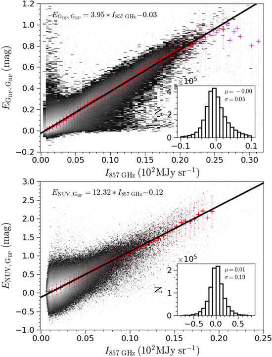
Figure 2. Linear fitting of the color excess  to the Planck/857 GHz intensity I857GHz(102MJy sr−1) (top) and
  to I857GHz(102MJy sr−1) (bottom). The grayscale decodes the source density, the red and magenta crosses denote the median values of each bin with small and large deviations from the linear fitting line (see Section 3.1.1 for details). The inset shows the distribution of the residuals with its median and standard deviation.
Download figure:
Standard image High-resolution image3.1.2. Selection of the Reference and Cloud Region
The denser MCs are supposed to have higher infrared intensity than the reference region so that the areas can be determined according to the Planck/857 GHz intensity. At first, both the reference and cloud region are searched for in a square area with a side length of four times the cloud's equivalent angular diameter ( ) centered at the cloud position. However, I857GHz does not decrease significantly within this area in many cases. So, the region is expanded to m times of the cloud's angular diameter until an appropriate region can be found for reference. The technical route of selecting the areas is illustrated by taking three typical cases (MBM 5, MBM 109, and MBM 40) as examples in Figure 3.
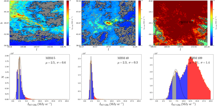
Figure 3. The studied area (top) and histogram (bottom) of I857GHz(MJy sr−1) in MBM 5 (left), MBM 40 (middle), and MBM 109 (right). In the studied area, the gray filled region bordered by a black dashed line is the background region, and the green–yellow–red region bordered by the red dashed line region inside the MBM cloud region (black solid line) is the cloud region. In the histogram, the black dashed curve is the local Gaussian fit, where the blue bars represent the noise (left) and transition (right) region, the gray bars represent the background region sources and the red bars represent the cloud region sources.
Download figure:
Standard image High-resolution imageThe distribution of the small peak is fitted by a Gaussian function to determine the median (μ) and the standard deviation (σ) of I857GHz for the reference region; then, the region with I857GHz in the range of μ − σ to μ is selected as the reference region, denoted by the black dashed line and gray histogram in the upper and lower panels, respectively, of Figure 3, and the region with I857GHz above μ + 3σ (the red dashed line and histogram in the upper and lower panels, respectively, of Figure 3) and inside the MBM-assigned MC area (marked by the black solid-line ellipse) is selected as the cloud region.
MBM 5 is a relatively isolated object for which the reference region can be found in an area four times as big as the cloud area. But MBM 109 is located within a large high-I857GHz area toward the sight line of the Tau–Per–Aur complex cloud so that the reference area has to be found in a far area; specifically, the area is expanded to 16 times the cloud's angular diameter. MBM 40 is taken as an example because it will be shown later that its distance is only 63 pc, which might put it inside the Local Bubble or right at the boundary of the Local Bubble. It can be seen that the values of μ and σ depend on the property and location of the MC. In this way, the reference and cloud area is defined for each cloud in an area specified by the m value listed in Table 1.
Table 1. The Distances and Color Excesses of the Molecular Clouds
| Cloud a | la | ba | dZucker b | dSchlafly c | dthis work d |
 d
d
|
 d
d
|
 d
d
| m d |
 d
d
|
 d
d
|
 d
d
| CERs d |
|---|---|---|---|---|---|---|---|---|---|---|---|---|---|
| (°) | (°) | (pc) | (pc) | (pc) | (mag) | (pc) | (mag) | (mag) | (pc) | (mag) | |||
| (1) | (2) | (3) | (4) | (5) | (6) | (7) | (8) | (9) | (10) | (11) | (12) | (13) | |
| MBM 1 | 110.19 | −41.229 | 265 | 228 | 285 ± 9.0 | 0.07 ± 0.0005 | 146 ± 8.7 | 0.09 ± 0.0022 | 8.0 | 0.20 ± 0.0155 | 296 ± 81.3 | 0.32 ± 0.0278 | 3.81 |
| MBM 3 | 131.291 | −45.676 | 314 | 277 | 309 ± 1.4 | 0.07 ± 0.0003 | 193 ± 3.8 | 0.11 ± 0.0010 | 4.0 | 0.20 ± 0.0036 | 185 ± 16.2 | 0.40 ± 0.0082 | 3.96 |
| MBM 4 | 133.515 | −45.303 | 286 | 269 | 320 ± 8.0 | 0.08 ± 0.0014 | 274 ± 14.6 | 0.13 ± 0.0013 | 4.0 | 0.22 ± 0.0133 | 104 ± 44.2 | 0.44 ± 0.0183 | 3.92 |
| MBM 5 | 145.967 | −49.074 | 279 | 187 | 297 ± 2.3 | 0.08 ± 0.0003 | 225 ± 3.1 | 0.14 ± 0.0012 | 4.0 | 0.23 ± 0.0051 | 260 ± 19.7 | 0.46 ± 0.0188 | 3.51 |
| MBM 6 | 145.065 | −39.349 | 111 | 151 | 153 ± 0.9 | 0.10 ± 0.0003 | 164 ± 2.7 | 0.23 ± 0.0017 | 8.0 | 0.28 ± 0.0054 | 179 ± 19.2 | 0.63 ± 0.0251 | 2.96 |
| MBM 7 | 150.429 | −38.074 | 171 | 148 | 213 ± 26.2 | 0.11 ± 0.0003 | 183 ± 2.1 | 0.20 ± 0.0026 | 10.0 | 0.31 ± 0.0039 | 156 ± 12.1 | 0.63 ± 0.0188 | 3.28 |
| MBM 8 | 151.75 | −38.669 | 255 | 199 | 262 ± 0.2 | 0.17 ± 0.0007 | 176 ± 3.5 | 0.26 ± 0.0028 | 12.0 | 0.48 ± 0.0106 | 108 ± 22.6 | 0.76 ± 0.0742 | 3.25 |
| MBM 9 | 156.531 | −44.722 | 262 | 246 | 248 ± 36.1 | 0.14 ± 0.0011 | 223 ± 7.7 | 0.08 ± 0.0034 | 4.0 | 0.38 ± 0.0282 | 277 ± 67.3 | 0.35 ± 0.0440 | 4.07 |
| MBM 11 | 157.983 | −35.06 | 250 | 185 | 147 ± 101.7 | 0.11 ± 0.0016 | 198 ± 14.2 | 0.33 ± 0.0037 | 16.0 | ||||
| MBM 12 | 159.351 | −34.324 | 252 | 234 | 278 ± 61.8 | 0.16 ± 0.0008 | 155 ± 5.3 | 0.51 ± 0.0181 | 4.0 | 0.49 ± 0.0123 | 201 ± 23.5 | 0.99 ± 0.0451 | 3.56 |
| MBM 13 | 161.591 | −35.89 | 237 | 191 | 409 ± 0.5 | 0.17 ± 0.0011 | 177 ± 4.7 | 0.42 ± 0.0108 | 12.0 | 0.48 ± 0.0162 | 155 ± 23.3 | 0.70 ± 0.0631 | 3.24 |
| MBM 14 | 162.458 | −31.861 | 275 | 233 | 295 ± 0.4 | 0.22 ± 0.0009 | 212 ± 2.8 | 0.27 ± 0.0006 | 2.0 | 0.69 ± 0.0058 | 259 ± 7.6 | 0.99 ± 0.0168 | 3.61 |
| MBM 15 | 191.666 | −52.294 | 200 | 160 | 164 ± 120.7 | 0.07 ± 0.0009 | 191 ± 10.2 | 0.11 ± 0.0038 | 5.0 | 0.17 ± 0.0136 | 152 ± 72.3 | 0.22 ± 0.0495 | 1.96 |
| MBM 16 | 170.603 | −37.273 | 170 | 147 | 210 ± 28.4 | 0.16 ± 0.0004 | 233 ± 2.5 | 0.64 ± 0.0057 | 10.0 | 0.47 ± 0.0075 | 246 ± 15.8 | 1.45 ± 0.0442 | 3.15 |
| MBM 17 | 167.526 | −26.606 | 130 | 165 | 231 ± 38.6 | 0.22 ± 0.0012 | 260 ± 5.4 | 0.30 ± 0.0072 | 4.0 | ||||
| MBM 18 | 189.105 | −36.016 | 155 | 166 | 149 ± 1.9 | 0.08 ± 0.0007 | 333 ± 8.4 | 0.41 ± 0.0022 | 12.0 | 0.21 ± 0.0056 | 336 ± 28.4 | 1.10 ± 0.0148 | 3.09 |
| MBM 19 | 186.041 | −29.929 | 143 | 156 | 293 ± 0.2 | 0.08 ± 0.0008 | 368 ± 10.3 | 0.34 ± 0.0075 | 72.0 | ||||
| MBM 22 | 208.091 | −27.477 | 266 | 238 | 181 ± 1.2 | 0.06 ± 0.0114 | 388 ± 137.2 | 0.11 ± 0.0047 | 2.0 | ||||
| MBM 23 | 171.835 | 26.706 | 349 | 305 | 252 ± 182.1 | 0.10 ± 0.0008 | 395 ± 10.1 | 0.07 ± 0.0052 | 10.0 | 0.31 ± 0.0167 | 470 ± 70.3 | 0.27 ± 0.0619 | 5.75 |
| MBM 24 | 172.272 | 26.965 | 351 | 279 | 338 ± 0.9 | 0.10 ± 0.0010 | 368 ± 13.0 | 0.11 ± 0.0015 | 4.0 | 0.32 ± 0.0224 | 490 ± 77.1 | 0.43 ± 0.0273 | 4.42 |
| MBM 25 | 173.752 | 31.475 | 342 | 297 | 362 ± 2.1 | 0.06 ± 0.0007 | 317 ± 12.2 | 0.07 ± 0.0008 | 4.0 | 0.15 ± 0.0101 | 410 ± 83.5 | 0.28 ± 0.0106 | 4.06 |
| MBM 34 | 2.307 | 35.7 | 117 | 110 | 178 ± 43.3 | 0.06 ± 0.0004 | 107 ± 8.2 | 0.14 ± 0.0022 | 14.0 | 0.14 ± 0.0092 | 174 ± 69.1 | 0.37 ± 0.0283 | 2.76 |
| MBM 35 | 6.571 | 38.128 | 86 | 89 | 296 ± 10.4 | 0.19 ± 0.0016 | 150 ± 9.5 | 0.23 ± 0.0066 | 4.0 | ||||
| MBM 36 | 4.229 | 35.792 | 107 | 105 | 99 ± 10.6 | 0.10 ± 0.0006 | 176 ± 5.8 | 0.42 ± 0.0013 | 8.0 | 0.34 ± 0.0139 | 234 ± 38.0 | 0.94 ± 0.0356 | 3.05 |
| MBM 37 | 6.067 | 36.757 | 115 | 121 | 143 ± 0.4 | 0.11 ± 0.0013 | 83 ± 13.7 | 0.32 ± 0.0011 | 4.0 | 0.34 ± 0.0290 | 107 ± 41.5 | 0.80 ± 0.0649 | 2.60 |
| MBM 38 | 8.222 | 36.338 | 92 | 77 | 286 ± 14.2 | 0.13 ± 0.0009 | 142 ± 7.6 | 0.52 ± 0.0399 | 12.0 | 0.40 ± 0.0186 | 108 ± 50.2 | 1.51 ± 0.0675 | 2.98 |
| MBM 40 | 37.57 | 44.667 | 93 | 64 | 63 ± 51.3 | 0.06 ± 0.0003 | 122 ± 6.4 | 0.14 ± 0.0013 | 8.0 | 0.17 ± 0.0046 | 217 ± 26.1 | 0.39 ± 0.0123 | 2.92 |
| MBM 49 | 64.496 | −26.539 | 212 | 204 | 330 ± 2.1 | 0.09 ± 0.0006 | 172 ± 10.0 | 0.13 ± 0.0014 | 2.0 | 0.24 ± 0.0112 | 179 ± 55.3 | 0.29 ± 0.0258 | 3.09 |
| MBM 51 | 73.313 | −51.526 | 190 ± 9.2 | 0.07 ± 0.0007 | 100 ± 9.0 | 0.06 ± 0.1058 | 12.0 | 0.25 ± 0.0233 | 272 ± 94.6 | 0.14 ± 0.0825 | 1.64 | ||
| MBM 53 | 93.965 | −34.058 | 259 | 253 | 266 ± 0.7 | 0.07 ± 0.0003 | 204 ± 6.3 | 0.18 ± 0.0013 | 8.0 | 0.20 ± 0.0071 | 285 ± 36.9 | 0.85 ± 0.0154 | 4.21 |
| MBM 54 | 91.624 | −38.103 | 245 | 231 | 238 ± 18.5 | 0.06 ± 0.0005 | 159 ± 7.2 | 0.15 ± 0.0028 | 10.0 | 0.14 ± 0.0044 | 163 ± 35.6 | 0.53 ± 0.0137 | 4.03 |
| MBM 55 | 89.19 | −40.936 | 245 | 206 | 266 ± 1.5 | 0.06 ± 0.0004 | 152 ± 6.9 | 0.15 ± 0.0007 | 4.0 | 0.15 ± 0.0069 | 244 ± 54.2 | 0.22 ± 0.0207 | 3.88 |
| MBM 56 | 103.075 | −26.06 | 265 | 227 | 271 ± 46.4 | 0.11 ± 0.0006 | 173 ± 6.5 | 0.19 ± 0.0024 | 4.0 | 0.33 ± 0.0098 | 163 ± 40.1 | 0.58 ± 0.0714 | 2.52 |
| MBM 101 | 158.191 | −21.412 | 289 | 283 | 288 ± 0.2 | 0.26 ± 0.0004 | 194 ± 1.8 | 0.60 ± 0.0012 | 8.0 | 0.81 ± 0.0043 | 245 ± 5.3 | 1.36 ± 0.0738 | 2.54 |
| MBM 102 | 158.561 | −21.154 | 289 | 275 | 289 ± 0.1 | 0.25 ± 0.0004 | 201 ± 1.6 | 0.59 ± 0.0010 | 8.0 | 0.79 ± 0.0040 | 248 ± 6.0 | 1.19 ± 0.0480 | 2.56 |
| MBM 103 | 158.885 | −21.552 | 279 | 269 | 285 ± 0.1 | 0.25 ± 0.0006 | 196 ± 3.3 | 0.49 ± 0.0009 | 8.0 | 0.78 ± 0.0041 | 235 ± 5.5 | 1.18 ± 0.0368 | 3.13 |
| MBM 104 | 158.405 | −20.436 | 281 | 262 | 291 ± 0.1 | 0.28 ± 0.0007 | 194 ± 3.4 | 0.69 ± 0.0007 | 5.0 | 0.95 ± 0.0110 | 243 ± 11.4 | 1.09 ± 0.0628 | 2.11 |
| MBM 105 | 169.52 | −20.126 | 127 | 139 | 142 ± 0.4 | 0.20 ± 0.0003 | 178 ± 1.6 | 0.27 ± 0.0005 | 5.0 | 0.61 ± 0.0073 | 192 ± 13.3 | 0.62 ± 0.0134 | 2.52 |
| MBM 106 | 176.334 | −20.781 | 158 | 190 | 179 ± 0.1 | 0.23 ± 0.0006 | 213 ± 2.4 | 0.40 ± 0.0005 | 16.0 | ||||
| MBM 107 | 177.654 | −20.343 | 141 | 197 | 142 ± 0.3 | 0.24 ± 0.0009 | 213 ± 3.5 | 0.48 ± 0.0007 | 16.0 | ||||
| MBM 108 | 178.238 | −20.342 | 143 | 168 | 139 ± 0.4 | 0.24 ± 0.0009 | 213 ± 2.8 | 0.48 ± 0.0014 | 16.0 | ||||
| MBM 109 | 178.93 | −20.1 | 155 | 160 | 176 ± 8.5 | 0.23 ± 0.0005 | 209 ± 2.1 | 0.38 ± 0.0012 | 16.0 | 0.72 ± 0.0038 | 241 ± 4.9 | 0.82 ± 0.0367 | 3.27 |
| MBM 110 | 207.598 | −22.944 | 356 | 313 | 300 ± 1.4 | 0.13 ± 0.0025 | 464 ± 19.5 | 0.12 ± 0.0009 | 4.0 | ||||
| MBM 111 | 208.547 | −20.222 | 400 | 366 | 403 ± 0.3 | 0.13 ± 0.0025 | 468 ± 21.2 | 0.30 ± 0.0011 | 4.0 | ||||
| MBM 115 | 342.331 | 24.146 | 141 | 137 | 126 ± 46.4 | 0.13 ± 0.0006 | 52 ± 2.4 | 0.28 ± 0.0015 | 8.0 | 0.37 ± 0.0143 | 76 ± 22.1 | 0.79 ± 0.0362 | 3.23 |
| MBM 116 | 342.715 | 24.506 | 137 | 134 | 158 ± 29.6 | 0.14 ± 0.0006 | 51 ± 1.6 | 0.29 ± 0.0015 | 8.0 | 0.39 ± 0.0134 | 70 ± 17.8 | 0.83 ± 0.0383 | 3.20 |
| MBM 117 | 343.001 | 24.085 | 138 | 140 | 141 ± 2.1 | 0.13 ± 0.0006 | 51 ± 1.3 | 0.23 ± 0.0014 | 8.0 | 0.40 ± 0.0164 | 86 ± 25.6 | 1.01 ± 0.0832 | 3.21 |
| MBM 118 | 344.018 | 24.758 | 140 | 56 | 146 ± 10.3 | 0.13 ± 0.0007 | 51 ± 1.9 | 0.27 ± 0.0021 | 8.0 | ||||
| MBM 119 | 341.613 | 21.396 | 169 | 150 | 111 ± 84.2 | 0.12 ± 0.0009 | 51 ± 1.0 | 0.11 ± 0.0024 | 8.0 | ||||
| MBM 120 | 344.231 | 24.188 | 135 | 59 | 145 ± 0.7 | 0.12 ± 0.0007 | 52 ± 2.1 | 0.28 ± 0.0022 | 8.0 | ||||
| MBM 123 | 343.281 | 22.121 | 143 | 101 | 75 ± 63.9 | 0.13 ± 0.0008 | 51 ± 1.0 | 0.22 ± 0.0035 | 8.0 | 0.50 ± 0.0592 | 197 ± 81.9 | 0.24 ± 0.0562 | 2.83 |
| MBM 124 | 343.966 | 22.725 | 145 | 89 | 147 ± 122.3 | 0.13 ± 0.0006 | 51 ± 0.9 | 0.14 ± 0.0098 | 8.0 | ||||
| MBM 125 | 355.536 | 22.541 | 129 | 115 | 131 ± 1.1 | 0.14 ± 0.0004 | 51 ± 1.6 | 0.30 ± 0.0026 | 21.0 | ||||
| MBM 127 | 355.409 | 20.877 | 146 | 147 | 150 ± 0.2 | 0.14 ± 0.0003 | 51 ± 1.3 | 0.89 ± 0.0070 | 21.0 | ||||
| MBM 128 | 355.562 | 20.592 | 136 | 134 | 150 ± 0.2 | 0.14 ± 0.0003 | 51 ± 1.4 | 0.89 ± 0.0067 | 21.0 | ||||
| MBM 129 | 356.155 | 20.761 | 139 | 141 | 145 ± 0.7 | 0.14 ± 0.0004 | 51 ± 47.5 | 0.52 ± 0.0033 | 21.0 | ||||
| MBM 130 | 356.805 | 20.265 | 129 | 109 | 150 ± 0.1 | 0.14 ± 0.0004 | 51 ± 1.3 | 0.60 ± 0.0042 | 21.0 | ||||
| MBM 131 | 359.156 | 21.787 | 158 | 106 | 161 ± 0.3 | 0.14 ± 0.0004 | 51 ± 1.2 | 0.48 ± 0.0027 | 21.0 | ||||
| MBM 133 | 359.176 | 21.37 | 161 | 98 | 240 ± 0.6 | 0.14 ± 0.0004 | 51 ± 1.2 | 0.57 ± 0.0052 | 21.0 | ||||
| MBM 134 | 0.132 | 21.782 | 158 | 121 | 285 ± 0.7 | 0.07 ± 0.0003 | 73 ± 8.1 | 0.46 ± 0.0062 | 24.0 | ||||
| MBM 136 | 1.271 | 20.992 | 139 | 120 | 110 ± 20.2 | 0.09 ± 0.0004 | 101 ± 4.6 | 0.42 ± 0.0027 | 21.0 | ||||
| MBM 145 | 8.482 | 21.842 | 108 | 152 | 185 ± 0.6 | 0.07 ± 0.0005 | 71 ± 12.6 | 0.49 ± 0.0024 | 16.0 | ||||
| MBM 146 | 8.784 | 22.035 | 116 | 179 | 197 ± 0.4 | 0.07 ± 0.0005 | 63 ± 8.6 | 0.46 ± 0.0058 | 16.0 | ||||
| MBM 148 | 7.543 | 21.066 | 156 | 116 | 186 ± 0.4 | 0.07 ± 0.0007 | 80 ± 14.4 | 0.55 ± 0.0023 | 16.0 | ||||
| MBM 151 | 21.533 | 20.93 | 138 | 122 | 145 ± 0.2 | 0.18 ± 0.0003 | 100 ± 1.9 | 0.31 ± 0.0006 | 8.0 | 0.53 ± 0.0042 | 107 ± 9.6 | 0.83 ± 0.0135 | 3.07 |
| MBM 152 | 359.48 | −20.474 | 86 ± 65.8 | 0.10 ± 0.0021 | 134 ± 16.0 | 0.15 ± 0.0024 | 4.0 |
Notes.
a The molecular cloud's series number (Column 1) and Galactic coordinates (Columns 2 and 3) retrieved from Magnani et al. (1985). b The distance and the error (Column 4) from Zucker et al. (2019). c The distance and the error (Column 5) from Schlafly et al. (2014). d The distance and the errors (Column 6), the foreground fitting parameters (Columns 7 and 8), and the color excess jump in the optical (Column 9), the multiples of the cloud's angular diameter (Column 10), the foreground fitting parameters (Columns 11 and 12), and the color excess jump (Column 13) in the optical-ultraviolet bands, and the color excess ratio of molecular clouds (Column 14) from this work.A machine-readable version of the table is available.
3.2. The Extinction-jump Model
Under the assumption that interstellar extinction increases smoothly with distance in the absence of any MCs, the extinction will make an upward jump at the distance of the cloud in the presence of an MC. In order to obtain accurate distance to and extinction of MCs, we take the extinction-jump model in Zhao et al. (2020), which is insensitive to the outliers. This model was designed originally by Zhao et al. (2018) and improved by Zhao et al. (2020) and used to determine the distance and the extinction of Galactic supernova remnants (SNRs). A similar model is used by Chen et al. (2017) and Yu et al. (2019) for other SNRs as well as MCs. The MCs cause the same effect as SNRs on the extinction and thus the extinction-jump model is applicable. In detail, the total extinction in terms of color excess E(d) toward the sight line of the MC is composed of two parts: the color excess of the cloud EMC(d), which dominates the total extinction, and the color excess of the diffuse interstellar medium EDISM(d),

Moreover, EMC(d) is described by an erf function,

where ΔEMC is the amplitude of the color excess jump, i.e.,  or
or  caused by the cloud, dc
is the distance to the center, and δ
d is the radius of the cloud calculated from dc
× θc
with θc
being the cloud's angular diameter.
caused by the cloud, dc
is the distance to the center, and δ
d is the radius of the cloud calculated from dc
× θc
with θc
being the cloud's angular diameter.
However, unlike Chen et al. (2017), Yu et al. (2019), and Zhao et al. (2020) which use a two-order polynomial function or root function, we use an exponential law to fit the color excess caused by the diffuse interstellar dust,

The function is modified to be in line with the high-latitude location of the MCs, in the sight line of which the material (including the interstellar dust) density falls exponentially with the vertical distance from the Galactic plane. Under this form, the parameter E0 reflects the cumulative color excess, and  with b being the latitude of the cloud is the scale height (h) of the dust disk in the sight line.
3.3. The Model Fitting
The model fitting is performed with the Markov Chain Monte Carlo procedure (Foreman-Mackey et al. 2013). In order to set the initial parameters very reasonably, a Markov chain is first run with 100 walkers and 250 steps. Then, the final chain uses the initial parameters with 100 walkers and 2000 steps, and we choose the last 1750 steps from each walker to sample the final posterior. The best estimates are the median values (50th percentile) of the posterior distribution and the uncertainties are derived from the 16th and 84th percentile values.
The variation of stellar extinction with distance is fitted separately for the reference region and the cloud region. Because the sample becomes more and more incomplete with distance, only the objects closer than 2000 pc with relative distance uncertainty <30% are taken into account. The fitting steps are in the following order: (1) fitting the optical extinction–distance measurements, i.e., the  versus d points of the reference region, by Equation (3) to obtain the parameters
  and
and  to describe the change of
  with d in the reference region. (2) Fitting the optical extinction–distance measurements of the cloud region by Equations (1) and (2) after substituting the above values of
  and
and  into Equation (1), which yields the distance dc
and the optical jump
into Equation (1), which yields the distance dc
and the optical jump  of the MC. (3) The same as step (1) but replacing
  by the
  of the reference region sources to obtain
  and
and  . (4) Similar to step (2), but replacing the optical parameters by ultraviolet values, i.e.,
  by
by  and
and  and
and  by
by  and
and  . In addition, the value of dc
resulting from the optical color excess is adopted rather than fitted because the number of measurements in the UV band is only about a quarter in the visual, thus only the jump
. In addition, the value of dc
resulting from the optical color excess is adopted rather than fitted because the number of measurements in the UV band is only about a quarter in the visual, thus only the jump  is derived in this step.
The model fitting for MBM 5, MBM 40, and MBM 109 with the reference and cloud sources are displayed as the example in Figures 4 and 5 for  and
and  , respectively. The green dots denote the sources in the reference region used to determine the variation of extinction with distance in the diffuse medium, and the red dots denote the sources in the cloud region used to determine the distance and extinction of the cloud. The key parameters with the uncertainty derived from modeling are shown in the upper-left corner of the figures (an extended version of Figure 4 is available for all the sample clouds).

Figure 4.
The fitting to the color excess,  , variation with the distance to the stars in the reference (green dots) and the cloud (red dots) region for the three typical clouds MBM 5, MBM 40, and MBM 109 with the extinction−distance model (Equations (1), (2), and (3). The parameters derived are shown in the upper-left corner, where "d" is the distance, "ΔE" is the color excess jump (
 ), and E0 and
  are the foreground parameters of the molecular cloud (
 and
and  ). (An extended version of this figure for all the studied clouds is available online). (The complete figure set (11 images) is available.)
Download figure:
Standard image High-resolution image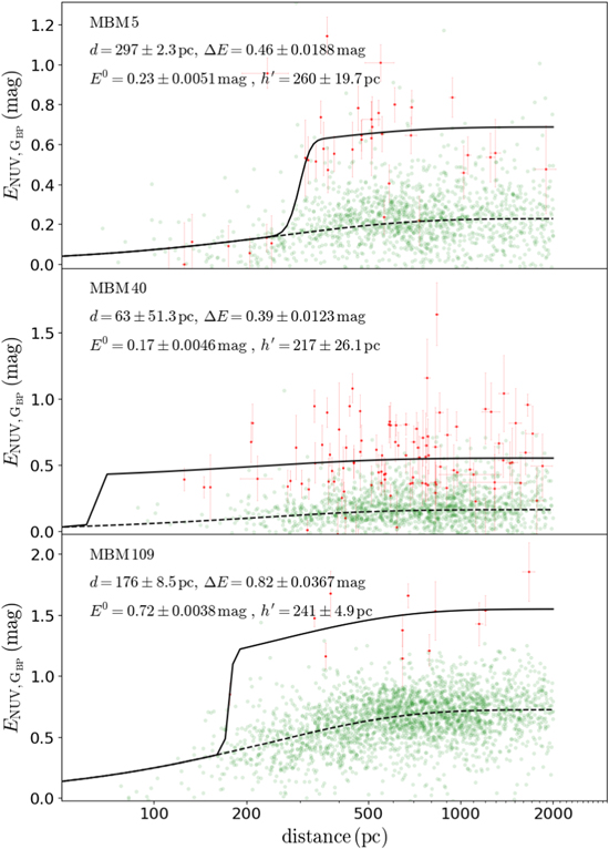
Figure 5. The same as Figure 4, but for  .
.
Download figure:
Standard image High-resolution image4. Results and Discussions
4.1. The Distance
The distance is derived for 66 of the 75 MBM clouds toward whose sight line more than three stars are present with an optical color excess measurement and lying behind the MC. The derived parameters are tabulated in Table 1. The distribution of the distances and their uncertainties is shown in Figure 6 where the symbols follow the convention in Figure 4. A simple visual inspection would conclude that the fitting agrees very well with the measurements in most cases. Meanwhile, the distances to G37.57−35.06 (MBM 11), G157.98+44.67 (MBM 40), G341.61+21.40 (MBM 119), G343.28+22.12 (MBM 123), and G359.48−20.47 (MBM 152) seem to be underestimated because there are few sources at a very close distance. As mentioned earlier, MBM 40 is the nearest with a distance of only 63 ± 51 pc, which puts it inside the Local Bubble or right at the boundary of the Local Bubble, if true. Though the uncertainty is large, the best value is consistent with that of Schlafly et al. (2014). On the other hand, this value is smaller than the 93 pc obtained by Zucker et al. (2019). Indeed, Figures 4 and 5 indicate that the first stars that show a marked increase in color excess have a distance of about 125 pc, apparently much larger, though still within the range of the uncertainty. These cases indicate that a precise distance from our method needs a continuous distribution of the distance of the tracers, in particular around the jump point. For MBM 40, more objects in front of the cloud should be measured to confirm its close distance.
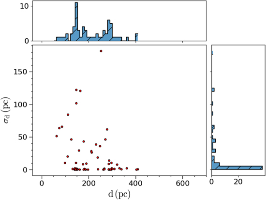
Figure 6. The distribution of the distances (d) and their uncertainties (σd ).
Download figure:
Standard image High-resolution imageFigure 7 shows the distance d and the vertical distance to the Galactic plane ∣z∣ versus the Galactic latitude ∣b∣. There is no systematic trend of d with ∣b∣ expected as these clouds are local, while ∣z∣ increases with the Galactic latitude ∣b∣.

Figure 7. The distance d (upper panel) and the Galactic disk distance ∣z∣ (lower panel) versus the Galactic latitude ∣b∣.
Download figure:
Standard image High-resolution imageThe distances to 9 of the 66 MCs were measured by Yan et al. (2019) and to 64 of them by Schlafly et al. (2014) and Zucker et al. (2019); these are compared with ours in Figure 8. It can be seen that the distances are more or less identical between the works at d < 200 pc. When d > 200 pc, this work yields a systematically larger distance than the others to a different extent in that the difference with Schlafly et al. (2014) is the largest and the difference with the other two works are mostly within the uncertainties. Comparing with these works, this work differs in a few aspects: (1) the intrinsic color indexes are derived from spectroscopy rather than photometry, (2) the stellar distance comes from the Gaia/EDR3 catalog instead of the DR2 catalog, (3) the model considers the thickness of the MC, and (4) the rise of the color excess of the foreground sources with distance is considered separately, which prevents the premature occurrence of jumps in some MCs. The first two factors improve the accuracy but should have no systematic influence on the distance.
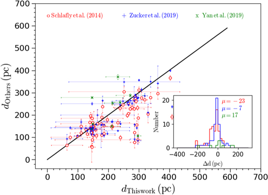
Figure 8. The comparison of the distances to molecular clouds with those obtained by Schlafly et al. (2014), Yan et al. (2019), and Zucker et al. (2019). The inset is the distribution of the differences with their results.
Download figure:
Standard image High-resolution image4.2. The Extinction
4.2.1. The Cloud
The extinction is determined for 66 MCs expressed by the optical color excess  and for 39 MCs by the UV-optical color excess
  . Their distribution along the latitude is shown in Figure 9 where the increase at low latitudes is visible as expected from their smaller vertical distance to the Galactic plane as evident in the lower panel of Figure 7. Meanwhile, it should be noted that the extinction appears large around ∣b∣ ∼ 35°−40°. The majority of
  is not bigger than 0.4 mag, i.e., AV ∼ 0.8 mag, and some clouds cause a large extinction but still smaller than AV ∼ 3 mag. Therefore, most of the clouds may be classified as translucent, and some of them as diffuse MCs.

Figure 9. The change of  and
and  with the Galactic latitude ∣b∣.
Download figure:
Standard image High-resolution imageIt should be noted that there are some stars with a large color excess, which is not reflected in the fitting parameters. The cross-identification with the Lynds dark clouds (Lynds 1962) finds that 24 MBM clouds contain 20 Lynds dark clouds, which are listed in Table 2. Some MBM clouds cover multiple Lynds clouds while some Lynds clouds repetitively appear in various MBM clouds. Such confusion implies that the boundary of a cloud needs to be redefined and will be considered in our next work. Figure 10 shows the maximum stellar  , i.e.,
  behind each MBM cloud identifiable in the Lynds dark clouds catalog in comparison with all the other clouds, where the blue asterisks denote the MBM MC containing some Lynds dark cloud(s). It can be seen that the majority of these clouds have
  , i.e., AV > 2.0 mag. Because dark clouds are normally defined to have AV > 5 mag, this is not consistent with the expectation for a dark cloud. It is likely that an interstellar cloud might have an average extinction of 2 mag with small patches having extinctions of 5 mag or more and so, on the basis of these small patches, the cloud is defined as a dark cloud while its average extinction is more like that of a translucent cloud. Meanwhile, a few clouds have AV ∼ 1.0–2.0 mag, smaller than the extinction that a dark cloud should have. One possible reason is that the stars that suffer serious extinction may become too faint to be observable by the LAMOST or GALAH spectroscopy survey. This also shows that the method in this work derives the median rather than the highest extinction of a cloud so that it is more appropriate for relatively large clouds than smaller dense clouds. Additionally, several MBM clouds have no associated Lynds dark clouds but with
  , AV < 3.0 mag is still an acceptable extinction for a translucent cloud though we cannot exclude the possibility of the presence of some dark nebula.

Figure 10. The change of maximum extinction  in the sight line of molecular clouds with the Galactic latitude ∣b∣. The blue and red asterisks are the result of MBM clouds with or without Lynds dark cloud.
Download figure:
Standard image High-resolution imageTable 2. MBM Molecular Clouds Associated with Lynds Dark Cloud
| MBM a | LDN a | AreaMBM b |
 b
b
|
 c
c
|
 c
c
|
|---|---|---|---|---|---|
| (deg2) | (deg2) | (mag) | (mag) | ||
| MBM 12 | LDN 1453 | 1.767 | 0.066 | 1.84 | 1.528 |
| MBM 12 | LDN 1454 | 1.767 | 0.86 | 1.84 | 1.84 |
| MBM 12 | LDN 1457 | 1.767 | 0.262 | 1.84 | 1.786 |
| MBM 12 | LDN1458 | 1.767 | 0.056 | 1.84 | 1.113 |
| MBM 18 | LDN 1569 | 2.836 | 0.631 | 1.009 | 0.855 |
| MBM 36 | LDN 134 | 1.767 | 0.22 | 1.183 | 1.109 |
| MBM 37 | LDN 169 | 1.227 | 0.86 | 1.612 | 1.612 |
| MBM 37 | LDN 183 | 1.227 | 0.24 | 1.612 | 1.612 |
| MBM 101 | LDN 1452 | 1.767 | 1.66 | 1.945 | 1.945 |
| MBM 101 | LDN 1448 | 1.767 | 0.053 | 1.945 | 1.296 |
| MBM 101 | LDN 1451 | 1.767 | 0.14 | 1.945 | 1.569 |
| MBM 102 | LDN 1448 | 1.767 | 0.053 | 1.945 | 1.296 |
| MBM 102 | LDN 1451 | 1.767 | 0.14 | 1.945 | 1.569 |
| MBM 102 | LDN 1452 | 1.767 | 1.66 | 1.945 | 1.945 |
| MBM 103 | LDN 1451 | 1.767 | 0.14 | 1.885 | 1.569 |
| MBM 103 | LDN 1448 | 1.767 | 0.053 | 1.885 | 1.296 |
| MBM 103 | LDN 1452 | 1.767 | 1.66 | 1.885 | 1.945 |
| MBM 104 | LDN 1452 | 1.767 | 1.66 | 2.387 | 1.945 |
| MBM 107 | LDN 1543 | 1.767 | 0.09 | 1.732 | 1.732 |
| MBM 107 | LDN 1546 | 1.767 | 0.37 | 1.732 | 1.842 |
| MBM 108 | LDN 1543 | 1.767 | 0.09 | 2.018 | 1.732 |
| MBM 108 | LDN 1546 | 1.767 | 0.37 | 2.018 | 1.842 |
| MBM 109 | LDN 1546 | 1.767 | 0.37 | 2.018 | 1.842 |
| MBM 110 | LDN 1634 | 1.767 | 0.492 | 0.773 | 0.466 |
| MBM 111 | LDN 1640 | 1.767 | 0.018 | 1.379 | 0.005 |
| MBM 125 | LDN 1721 | 1.767 | 0.287 | 0.769 | 0.424 |
| MBM 126 | LDN 1719 | 1.767 | 0.61 | 1.218 | 1.218 |
| MBM 127 | LDN 1719 | 1.767 | 0.61 | 1.218 | 1.218 |
| MBM 128 | LDN 1719 | 1.767 | 0.61 | 1.218 | 1.218 |
| MBM 129 | LDN 1719 | 1.767 | 0.61 | 1.218 | 1.218 |
| MBM 130 | LDN 1752 | 1.767 | 1.78 | 0.979 | 1.421 |
| MBM 131 | LDN 1781 | 1.767 | 1.19 | 0.778 | 0.778 |
| MBM 133 | LDN 1781 | 1.767 | 1.19 | 0.778 | 0.778 |
| MBM 134 | LDN 1781 | 1.767 | 1.19 | 0.559 | 0.778 |
| MBM 145 | LDN 234 | 1.767 | 1.41 | 0.648 | 0.802 |
| MBM 148 | LDN 234 | 1.767 | 1.41 | 0.802 | 0.802 |
Notes.
a The molecular cloud's series number (Columns 1 and 2) from Magnani et al. (1985) (MBM) and Lynds (1962) (LDN). b The cloud area (Columns 3 and 4) from MBM and LDN. c The maximum color excess in the cloud region (Columns 5 and 6) from MBM and LDN.
A machine-readable version of the table is available.
Download table as: DataTypeset image
4.2.2. The Reference Region
The reference region is selected from the low-intensity noise-like emission at Planck/857 GHz, representative of the diffuse interstellar medium. Our model for the reference extinction by Equation (3) assumes an exponential disk with vertical height. The parameter E0 in Equation (3) is the cumulative extinction and  is the scale height of the extinction/dust disk toward the specific high-latitude sight line.
The relationship between the parameters from fitting  and
and  for the reference regions is shown in Figure 11. As shown in Figure 11(a), there is a good linear relationship between
  and
and  . The slope of the fitting line is 3.27, which reflects the ratio of the accumulated color excess of the diffuse interstellar medium in the UV and optical bands. This ratio is very close to the all-sky color excess ratio of 3.25 in Paper I.
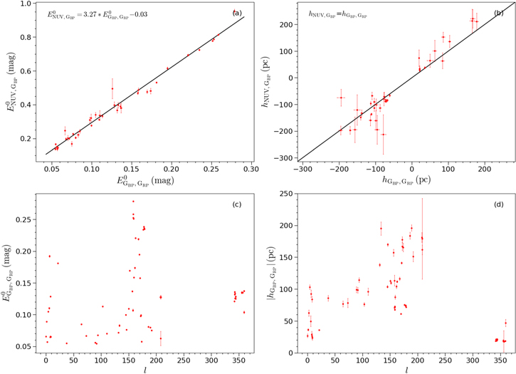
Figure 11. The relationship of  and
and  (top, left) and
  and
and  (top, right) as well as the distribution of
  (bottom, left) and
  (bottom, right). Red asterisks are the parameters of foreground and black line is the fitting line of
  and
and  (top, left) and
  =
=  line (top, right).
Download figure:
Standard image High-resolution imageAfter multiplying  and
and  by
by  , the dust disk scale height
  and
and  in the sight line is obtained. Figure 11 (b) presents the relation between
  and
and  , which are basically distributed near the equal line while some points deviate. Because the parameter
  is very sensitive to the data size,
  should be more reliable due to its much smaller error and more data points in the Gaia/EDR3 catalog. The change of
  and
and  with Galactic longitude is displayed in Figures 1
1(c) and 11(d). The scale height varies from about 50 to 250 pc, with an obvious increase toward the anticenter direction consistent with a flaring dust disk. This median thickness of about 100 pc indicates that the dust disk agrees with the thin gaseous disk of the Milky Way whose scale height ranges around 100–300 pc (e.g., Ferguson et al. 2017; Ma et al. 2017).
with Galactic longitude is displayed in Figures 1
1(c) and 11(d). The scale height varies from about 50 to 250 pc, with an obvious increase toward the anticenter direction consistent with a flaring dust disk. This median thickness of about 100 pc indicates that the dust disk agrees with the thin gaseous disk of the Milky Way whose scale height ranges around 100–300 pc (e.g., Ferguson et al. 2017; Ma et al. 2017).
The resultant  is compared with Schlegel et al. (1998, SFD98) for the reference region because
  is supposed to be the cumulative extinction along the sight line. The value of
  is first converted to
  for comparison (Niu et al. 2021). Figure 12 shows the linear fitting between
  and the median value of
  in each studied reference area. The slope is 0.95 and the intercept is −0.005, which means our result is very consistent with that of SFD98.

Figure 12. Comparison between  and
and  in the background region.
Download figure:
Standard image High-resolution image4.3. Dust Property of High-latitude Molecular Clouds
Because the extinction of an MC changes across the cloud, the overall average color excess of the cloud, i.e.,  and
and  , should be an extinction indicator of the overall cloud. However, the ratio
  of the cloud has great uncertainty, perhaps due to the very large dispersion in the extinction. Instead, the sources behind the cloud are all taken into consideration to determine the color excess ratio
  /
/ and then the dust property of an MC. By subtracting the color excess of the diffuse interstellar medium at equal distances from the color excess of these sources, the corresponding color excess of the MC in the sight line is obtained. Requiring the number of selected sources to be N ≥ 3, the color excess ratios of 39 MCs are calculated by linear fitting through iterative 3σ clipping (Paper I). The results of MBM 5, MBM 40, and MBM 109 are displayed in Figure 13, where
  and
and  have a good linear relationship.
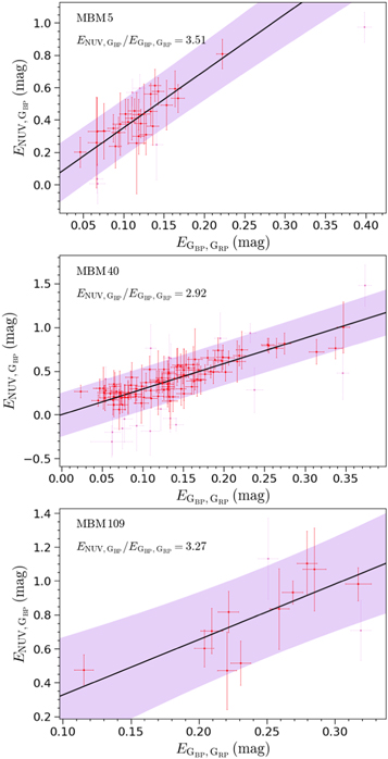
Figure 13. Linear fitting of the color excess  to
to  in MBM 5, MBM 40, and MBM 109. Red and magenta dots are sources in and out of the 95% confidence interval, the black line is the fitting curve, and the purple shadow is the 95% confidence interval.
Download figure:
Standard image High-resolution imageThe change of the color excess ratios ( ) with
  of these MCs is shown in the lower panel of Figure 14. Obviously, the color excess ratio of the MCs (red asterisks) increases at
  . As Paper I pointed out, there exists a systematic variation in both Teff and
  with the Galactic location for the tracing stars, which can shift the effective wavelength of the filters and then the color excess ratio
  in a complicated way (see Figure 10 of Paper I). In brief,
  generally decreases with
  when Teff > 6500 K, while increases with
  when Teff < 6500 K. On average, this color excess ratio is bigger for higher Teff. The upper panel of Figure 14 confirms that Teff changes with
  . In order to see the change of dust property, the effects of Teff and
  on the color excess ratio should be stripped off in advance. For this purpose, the color excess ratio of each is calculated assuming that only Teff and
  play a role, i.e., convolving the stellar emergent spectrum with the response curve of the filter and the F99 extinction curve at RV = 3.1 (Fitzpatrick 1999) to get the color excess ratio at the corresponding effective wavelength. The derived color excess ratio is represented by blue asterisks in Figure 14, which agrees with the expectation from Paper I that the lower Teff around 6000 K in combination with the smaller
  should lead to a smaller
  . The observed trend that the color excess ratio of the MCs increases at smaller
  is thus in the opposite direction. It seems that this trend can only be explained by the change of dust property at small extinction. In principle, the color excess ratio is sensitive to the composition and size distribution of the dust particles (Draine 2011). Larson & Whittet (2005) conclude that many high-latitude clouds have enhanced abundances of relatively small grains based on the near-infrared extinction curves. The enhanced proportion of small grains can also explain the observed ratio variation of the near-ultraviolet-to-visual extinction here. Indeed, this trend is already found in the whole high-latitude sky in Paper I and now confirmed by this work.
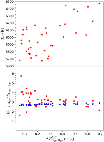
Figure 14. The change of Teff (upper panel) and color excess ratios  /
/ (lower panel) with
  . Red asterisks are the results of the studied molecular clouds, while the blue asterisks are the simulation results considering the effective wavelength shift because of Teff and
  (see Paper I for details).
Download figure:
Standard image High-resolution image5. Summary
This work uses the color excesses of more than 4 million stars in the visual and 1 million stars in the ultraviolet to explore the high-latitude MCs cataloged by Magnani et al. (1985). The cloud and reference region are selected from the Planck/857 GHz image in order to clarify the extinction caused by the cloud. The distances to 66 clouds are determined by the extinction jump along the sight line caused by the cloud denser than the diffuse area.
The major results of this paper are as follows:
- 1.The cumulative color excess
 of the diffuse ISM and scale height hvisible of the dust disk is derived for 66 areas, while the cumulative color excess of the diffuse ISM is obtained for 39 areas. The calculated scale height is around 50–250 pc, which agrees with the thin gaseous disk of the Milky.
 - 2.
- 3.The color excess ratio of 39 MCs is calculated and found to be obviously larger at lower extinction, which cannot be interpreted as the shift of the effective wavelength because of the variation in Teff and . This indicates that the MCs with lower extinction have more small dust particles.


We thank Profs. Jian Gao and Haibo Yuan, and Mr. Ye Wang and Bin Yu for discussions. We are also grateful to the referee for helpful suggestions. This work is supported by CMS-CSST-2021-A09, National Key R&D Program of China No. 2019YFA0405503, and NSFC 11533002. H.Z. is funded by the China Scholarship Council (No. 201806040200). This work made use of the data taken by GALEX, LAMOST, Gaia, and GALAH, MBM.
Facilities: GALEX - Galaxy Evolution Explorer satellite, LAMOST - , Gaia - , GALAH - , MBM - .