


ABSTRACT
We substantially update the capabilities of the open-source software instrument Modules for Experiments in Stellar Astrophysics (MESA). MESA can now simultaneously evolve an interacting pair of differentially rotating stars undergoing transfer and loss of mass and angular momentum, greatly enhancing the prior ability to model binary evolution. New MESA capabilities in fully coupled calculation of nuclear networks with hundreds of isotopes now allow MESA to accurately simulate the advanced burning stages needed to construct supernova progenitor models. Implicit hydrodynamics with shocks can now be treated with MESA, enabling modeling of the entire massive star lifecycle, from pre-main-sequence evolution to the onset of core collapse and nucleosynthesis from the resulting explosion. Coupling of the GYRE non-adiabatic pulsation instrument with MESA allows for new explorations of the instability strips for massive stars while also accelerating the astrophysical use of asteroseismology data. We improve the treatment of mass accretion, giving more accurate and robust near-surface profiles. A new MESA capability to calculate weak reaction rates "on-the-fly" from input nuclear data allows better simulation of accretion induced collapse of massive white dwarfs and the fate of some massive stars. We discuss the ongoing challenge of chemical diffusion in the strongly coupled plasma regime, and exhibit improvements in MESA that now allow for the simulation of radiative levitation of heavy elements in hot stars. We close by noting that the MESA software infrastructure provides bit-for-bit consistency for all results across all the supported platforms, a profound enabling capability for accelerating MESA's development.
Export citation and abstract BibTeX RIS
1. INTRODUCTION
The development of a relatively complete and quantitative picture of stellar evolution is one of the great drivers of astrophysics. On the observational side of this impetus, the Kepler (Borucki et al. 2010) and CoRoT (Baglin et al. 2009) missions continuously monitored more than 100,000 stars in a 100 deg2 window with a dynamic range of apparent stellar brightness of 106. Highlights include the discoveries that nearly all γ Doradus and δ Scuti stars are hybrid pulsators, and the detection of solar-like oscillations in a large sample of red giants (Auvergne et al. 2009; De Ridder et al. 2009; Bedding et al. 2010; Grigahcène et al. 2010; Christensen-Dalsgaard & Thompson 2011; Chaplin & Miglio 2013). The Dark Energy Survey is scanning 5000 deg2 of the southern sky in five optical filters every few days to discover and study thousands of supernovae (e.g., Papadopoulos et al. 2015; Yuan et al. 2015). Building upon the legacy of the Palomar Transient Factory (Law et al. 2009), the intermediate Palomar Transient Factory conducts a fully automated, wide-field survey that systematically explores the transient sky with a 90 s to 5 days cadence (Vreeswijk et al. 2014). The forthcoming Zwicky Transient Facility will enable a survey more than an order of magnitude faster at the same depth as its predecessors. In its unique orbit, the Transiting Exoplanet Survey Satellite will have an unobstructed view to scrutinize the light curves of the brightest 100,000 stars with a 1 minute cadence (Ricker et al. 2015). The Gaia mission aims to provide unprecedented distance and radial velocity measurements with the accuracies needed to reveal the evolutionary state, composition, and kinematics of about one billion stars in our Galaxy (e.g., Creevey et al. 2015; Sacco et al. 2015). The Large Synoptic Survey Telescope will image the entire southern hemisphere deeply in multiple optical colors every week with its three billion pixel digital camera, thus opening a new window on transient objects such as interacting close binary systems. (e.g., Oluseyi et al. 2012).
Interpreting these new observations and predicting new stellar phenomena propels the theoretical side, in particular the evolution of the community software instrument Modules for Experiments in Stellar Astrophysics (MESA) for research and education. We introduced MESA in Paxton et al. (2011, hereafter Paper I) and expanded its range of capabilities in Paxton et al. (2013, hereafter Paper II). This paper describes the major new advances for MESA modeling of binary systems, shock hydrodynamics, explosions of massive stars and X-ray bursts with large, in situ reaction networks. Moreover it details the coupling of MESA with the non-adiabatic pulsation software instrument GYRE (Townsend & Teitler 2013). We also describe advances made to existing modules since Paper II, including improved treatments of mass accretion, weak reaction rates, and particle diffusion.
It has been a little more than 200 years since Herschel (1802) announced, after 25 years of observation, that certain pairs of stars displayed evidence of orbital motion around their common center of mass. Binary systems allow the masses of their component stars to be directly determined, which in turn allows stellar radii to be indirectly estimated. This allows the calibration of an empirical mass–luminosity relationship from which the masses of single stars can be estimated (Torres et al. 2010). Recent surveys such as Raghavan et al. (2010) suggest that 30%–50% of solar-like systems in the Galactic disk are composed of binaries, where the binary fraction is higher for more massive stars (Sana et al. 2012; Kobulnicky et al. 2014). As argued by de Mink et al. (2013), the most rapidly rotating massive stars are expected in binary systems as a consequence of accretion-induced spin-up. Differential rotation has a major impact on the evolution of massive stars (Heger et al. 2000, 2005; Maeder & Meynet 2000) and for single stars the corresponding physics has been included in MESA as described in Paper II. On the other hand, very few works that include the physics of differential rotation in binaries have been published (Petrovic et al. 2005; Cantiello et al. 2007). Our improvements to MESA now allow for the calculation of differentially rotating binary stars.
The rapid expansion of extra-solar planet research has led to a revival of interest in the detailed properties of stars probed through space-based brightness variability studies and radial velocity measurements. Stellar properties can be derived from measurements of the radial and non-radial oscillation modes of a star, but this requires the accurate and efficient computations of mode frequencies and their eigenfunctions enabled by the coupling of GYRE with MESA.
There are many ways  stars can end their lives (e.g., Woosley et al. 2002; Smartt 2009; Meynet et al. 2009; Langer 2012; Nomoto et al. 2013; Smith 2014). Some become electron capture supernovae; others collapse with most of their extended envelope intact and yield a Type II supernova; others can lead to pair instability; and some have envelopes thin enough to allow a jet to break through and appear as a long gamma-ray burst (MacFadyen & Woosley 1999; Woosley & Bloom 2006; Gehrels et al. 2009). There is a pressing need throughout the stellar community to routinely explore this entire mass range with new supernova progenitor and explosion models. The observational facilities discussed above have found explosions that indicate large amounts of mass are lost within a few years of explosion (Smith 2014); some show evidence of optically thick winds present at the moment of explosion (Ofek et al. 2014), while others have yet to be securely identified with a specific core collapse scenario. These mysteries, coupled with the community's call for new yields from massive stars for galactic chemical evolution studies motivate the development of implicit shock hydrodynamics and explosions with large, in situ reactions networks in MESA.
The paper is outlined as follows. Section 2 describes the new capability of MESA to evolve binary systems. Section 3 discusses the new non-adiabatic pulsation capabilities resulting from fully coupling to the GYRE software instrument. Section 4 describes the improvements to accommodate implicit hydrodynamics with shocks. New capabilities for advanced burning and X-ray bursts with large, in situ reaction networks are described in Section 5. In Section 6 we model the pre-supernova evolution of massive stars and combine the implicit hydrodynamics module and the new capabilities for advanced burning to probe the nucleosynthesis and yields of core-collapse supernovae. Section 7 discusses the improvements for a more robust and efficient treatment of mass accretion. Section 8 presents a new option for an on-the-fly calculation of weak reaction rates and their application to the Urca process and accretion-induced-collapse models. Section 9 presents improvements in the physics implementation of particle diffusion by including radiative levitation and pushing diffusion methods into the strongly coupled, electron degenerate regime. In Section 10 we discuss improvements to the MESA software infrastructure, highlighting bit-for-bit consistency across operating systems and compilers. We conclude in Section 11 by noting additional improvements to MESA are likely to occur in the near future. Important symbols are defined in Table 1. We denote components of MESA, such as modules and routines, in Courier font, e.g., evolve_star.
Table 1. Variable Index
| Name | Description | First Appears |
|---|---|---|
| a | Orbital seperation | 2.1 |
| A | Atomic mass number | 5 |
| α | Fine structure constant | 8.1 |
| c | Speed of light | 2.2.1 |
| e | Specific thermal energy | 4.4 |
| η | Wind mass loss coefficient | 6.1 |
| g | Gravitational acceleration | 5.3 |
| G | Gravitational constant | 2.1 |
| Γ | Coulomb coupling parameter | 9 |
| I | Moment of inertia | 2.4 |
| κ | Opacity | 1 |
| L | Luminosity | 4.4 |
| λ | Reaction rate | 5 |
| m | Lagrangian mass coordinate | 4 |
| M | Stellar mass | 2.1 |
| M1 | Donor mass | 2.1 |
| M2 | Accretor mass | 2.1 |
| μ | Mean molecular weight | 2.3.1 |
| N | Neutron number | 6.1 |

|
Dimensionless eigenfrequency | 3.1 |
| Ω | Angular frequency | 2.4 |
| Q | Nuclear rest mass energy difference | 8.1 |
| P | Pressure | 2.3.1 |
| q | Fractional mass coordinate | 7 |
| q1 | Mass ratio, 
|
2.3 |
| q2 | Mass ratio, 
|
2.3 |
| r | Radial coordinate | 2.3.1 |
| R | Stellar radius | 2.3 |
| ρ | Baryon mass density | 2.3.1 |
| s | Specific entropy | 7 |

|
Oscillation eigenfrequency | 3.1 |
| t | Time | 2.4 |
| T | Temperature | 2.3.1 |
| τ | Timescale | 2.4 |
| v | Velocity | 4.1 |
| X | Baryon mass fraction | 5 |
| Y | Molar abundance | 5 |

|
Gravitational redshift | 5.3 |
| Z | Atomic number | 5 |

|
Mixing length parameter | 3.1 |
| CP | Mass specific heat at constant pressure | 7 |

|

|
7 |

|

|
7 |
| dm | Mass of cell | 4.1 |

|
mass associated with cell face | 4.3 |
| dq | Fractional mass of cell | 7 |

|
Numerical timestep | 2.2.3 |

|
Change of stellar mass in one step | 7 |

|
Adiabatic temperature gradient 
|
7 |

|
Stellar temperature gradient 
|
7 |

|
Fermi energy | 6.1 |

|
Gravitational heating rate | 4.9 |

|
Neutrino energy loss rate | 4.9 |

|
Nuclear energy generation rate | 4.9 |

|
Viscous heating rate | 4.4 |

|
Artificial dynamic viscosity coefficient | 4.1 |

|
Convective overshoot parameter | 3.1 |

|
Viscous acceleration | 4.3 |

|
Radiative acceleration | 9.1.3 |

|
First adiabatic exponent 
|
2.3.1 |

|
Pressure scale height | 2.3 |

|
Rate of change of angular momentum | 2.2 |

|
Orbital angular momentum | 2.1 |

|
Boltzmann constant | 2.3.1 |

|
Mean inter-ion spacing | 9 |

|
Proton mass | 2.3.1 |

|
Accreted mass accumulated, 
|
7.2 |

|
Mass of unmodeled inert core | 7 |

|
 at time of nova runaway at time of nova runaway |
7.2 |

|
Eddington accretion rate | 2.1 |

|
Electron chemical potential | 8.1 |

|
Ion number density | 9 |

|
Linear oscillation frequency | 3.1 |

|
Orbital period | 2.1 |

|
Artificial viscosity energy | 4.2 |

|
Roche lobe radius | 2.3 |

|
Debye radius | 9.1.1 |

|
Central baryon mass density | 6 |
| t' | GR corrected time for observer at infinity | 5.3 |

|
Central temperature | 6 |

|
Effective temperature | 2.3.1 |

|
Timescale to accrete outer star layer | 7 |

|
Convective timescale | 4.7 |

|
Oscillation e-folding time | 3.1 |

|
Tidal synchronization timescale | 2.4 |

|
Thermal timescale of outer star layer | 7 |

|
Convection timescale | 4.5 |

|
Time centered velocity | 4.1 |

|
Electrons per baryon | 5 |
2. BINARIES
MESAbinary is a MESA module that uses MESAstar to evolve binary systems. It can be used to evolve a full stellar model plus a point mass companion or to simultaneously evolve the structure of two stars. It optionally allows the modeling of systems including stellar rotation, assuming the axis of rotation of each star to be perpendicular to the orbital plane, accounting for the effects of tidal interaction and spin-up through accretion. The implementation of MESAbinary benefits from early contributions by Madhusudhan et al. (2006) and Lin et al. (2011) who modeled mass transfer from a star to a point mass.
Here we provide an overview of the modeled physical processes for circular binary systems and describe the tests against which we validate MESAbinary.
2.1. Initialization of a Circular Binary System
A binary system is initialized by specifying the components and either the orbital period  or separation a. Each component can be a point mass or a stellar model. The initial model(s) are provided by a saved MESA model or a zero-age main-sequence (ZAMS) specification. For stellar models including rotation, the initial rotational velocities of each component can be explicitly defined, or set such that the star is synchronized to the orbit at the beginning of the evolution. The orbital angular momentum of the system is

where M1 and M2 are the stellar masses. Evolution of M1, M2, and  is used to update a using Equation (1). Masses can be modified both by Roche lobe overflow (RLOF) and winds. The total time derivatives of the component masses are given by

where M1 is the donor mass and M2 the accretor mass. The stellar wind mass loss rates are  and
and  (see Paper I and Paper II) and
  is the mass transfer rate from RLOF, all defined as negative. The factor
  represents the efficiency of accretion and can be used to limit accretion to the Eddington rate
  .
.
2.2. Evolution of Orbital Angular Momentum
To compute the rate of change of orbital angular momentum, we consider the contribution of gravitational waves, mass loss, magnetic braking, and spin–orbit (LS) coupling

from which the change in orbital angular momentum in one step is calculated as  , where
  is the timestep. Unless models with stellar rotation are being used, the
  term is equal to zero, and the contribution of the individual spins of each star is not directly considered. On the other hand, the
  term implicitly assumes a strong tide that keeps the orbit synchronized. The simultaneous usage of
  with stellar rotation is not consistent (see Section 2.2.4). We now describe how these terms are computed.
2.2.1. Gravitational Wave Radiation
Very compact binaries can experience significant orbital decay due to the emission of gravitational waves. Observations of the Hulse–Taylor binary pulsar over three decades (Weisberg & Taylor 2005) and of the double pulsar (Kramer et al. 2006) have tested the predicted effect from general relativity to a high precision. The angular momentum loss from gravitational waves is

2.2.2. Mass Loss
We assume the mass lost in a stellar wind has the specific orbital angular momentum of its star. For the case of inefficient mass transfer, angular momentum loss follows Soberman et al. (1997), where fixed fractions of the transferred mass are lost either as a fast isotropic wind from each star or a circumbinary toroid with a given radius:

where  ,
,  , and
, and  are respectively the fractions of mass transferred that is lost from the vicinity of the donor, accretor and circumbinary toroid, and
  is the radius of the toroid. Ignoring winds, the efficiency of mass transfer is then given by
  . When accretion is limited to
  , efficiency of accretion is given by

and the additional mass being lost is added to the  term in Equation (5), i.e., it is assumed to leave the system carrying the specific orbital angular momentum of the accretor.
2.2.3. Spin–Orbit Coupling
Tidal interaction and mass transfer can significantly modify the spin angular momentum of the stars in a binary system, acting as both sources and sinks for orbital angular momentum. The impact spin–orbit interactions have on orbital evolution depends on the orbital separation and the mass ratio, with the effect being greater for tighter orbits and uneven masses. The corresponding contribution to  is computed by demanding conservation of the total angular momentum, accounting for losses due to the other
  mechanisms and loss of stellar angular momentum due to winds.
In a fully conservative system, the change in orbital angular momentum in one timestep is  , where
  and
and  are the changes in spin angular momenta. This needs to be corrected if mass loss is included, as winds take away angular momentum from the system. If
  and
and  are the amounts of spin angular momentum removed in a step from each star due to mass loss (including winds and RLOF),

where the additional factor for the donor accounts for mass lost from the system, ignoring mass loss due to mass transfer. In the absence of RLOF this equation becomes symmetric between both stars, as then  .
.
The form of Equation (7) is independent of how tides and angular momentum accretion work, as it is merely a statement on angular momentum conservation. The details of how we model these processes and their impact on the spin of each component are described in Section 2.4.
2.2.4. Magnetic Braking
The rotational velocities of low mass stars are strongly correlated with their ages (Skumanich 1972). This spin-down arises from the coupling of the stellar wind to a magnetic field. If the star is in a binary system and tidally coupled to the orbit, magnetic braking can provide a very efficient sink for orbital angular momentum (Mestel 1968; Verbunt & Zwaan 1981). We implement this effect following Rappaport et al. (1983), who assumed the star being braked is tidally synchronized:

where in the simplest approximation  = 4 (Verbunt & Zwaan 1981). A similar contribution from the accretor can be included. As tidal synchronization is assumed, this formulation is incompatible with the use of LS coupling.
It is normally assumed that once a star becomes fully convective, the dynamo process that regenerates the field will stop working or at least behave in a qualitatively different manner. Similarly, magnetic fields in stars with radiative envelopes are of a significantly different nature than those seen in stars with convective envelopes, and there is no simple way to predict even the presence of magnetism (Donati & Landstreet 2009). By default, MESAbinary only accounts for magnetic braking as long as the star being braked has a convective envelope and a radiative core, though the process might still operate outside of these conditions.
2.3. Mass Transfer from RLOF
Close binary stars are defined as systems tight enough to interact through mass transfer, with the most important mechanism being RLOF. This process is commonly modeled in 1D by considering the spherical-equivalent Roche lobe radius  of each object (Eggleton 1983)
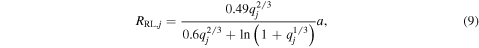
where j is the index identifying each star,  and
and  . This fit is correct up to a few percent for the full range of mass ratios,
  . Mass transfer occurs then when the radius of a star approaches or exceeds
  . Depending on several factors, once a star begins RLOF the ensuing mass transfer phase can proceed on a nuclear, thermal, or dynamical timescale.
The stability of mass transfer is normally understood in terms of mass–radius relationships (e.g., Soberman et al. 1997; Tout et al. 1997),


Here,  gives the radial response of the donor to mass loss when it happens slowly enough for the star to remain in thermal equilibrium. When mass loss proceeds on a timescale much shorter than the thermal timescale of the star, but still slow enough for the star to retain hydrostatic equilibrium then the radial response will be given by
  . The dependency of the Roche lobe radius on mass transfer is encoded in
  . In general
 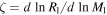 is a function of
  , so requiring
  will determine the value of
  . If an overflowing star satisfies
  , then it can remain inside its Roche lobe by transferring mass while retaining thermal equilibrium. If on the contrary
  , mass transfer will proceed on a thermal timescale, while for the extreme case
  the star will depart from hydrostatic equilibrium and the process will be dynamical. MESA cannot model common envelope or contact binaries.
MESAbinary provides both explicit and implicit methods to compute mass transfer rates. An explicit computation sets the value of  at the start of a step, while an implicit one begins with a guess for
  and iterates until the required tolerance is reached. The composition of accreted material is set to that of the donor surface, and the specific entropy of accreted material is the same as the surface of the accretor. In models with rotation the specific angular momentum of accreted material is described in Section 2.4.
2.3.1. Explicit Methods
MESAbinary implements two mass transfer schemes: the model of Ritter (1988) which we refer to as the Ritter scheme and Kolb & Ritter (1990) which we refer to as the Kolb scheme. We use the mass ratio q2 consistent with the Ritter scheme.
Ritter scheme: Stars have extended atmospheres therefore RLOF can take place through the L1 point even when  . Ritter (1988) estimated the mass transfer rate for this case as

where  is the pressure scale height at the photosphere of the donor and

where  is the proton mass,
  is the effective temperature of the donor, and
  and
and  are the mean molecular weight and density at its photosphere. The two fitting functions are

and
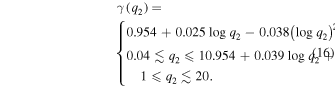
Outside the ranges of validity,  and
and  are evaluated using the value of q2 at the edge of their respective ranges.
Kolb scheme: Kolb & Ritter (1990) extended the Ritter scheme in order to cover the case  according to

where  is the first adiabatic exponent, and Pph and PRL are, respectively, the pressures at the photosphere and at the radius for which
  .
.
2.3.2. Implicit Methods
Explicit schemes exhibit large jumps in  unless the timestep is severely restricted. Therefore, if one needs accurate values of
  and stellar radius, this requires use of an implicit scheme. Implicit schemes also allow the calculation these quantities when there is no general closed form formula for
  .
.
These implicit methods use a bisection-based root solve to satisfy  at the end of the step, where ξ is a given tolerance. The implicit schemes are then defined by the choice of the function
  . For the Ritter and the Kolb scheme the function is chosen as

with  being the mass transfer rate computed at the end of each iteration.
A different implicit method is also provided. In this case, whenever the donor star overflows its Roche lobe the implicit solver will adjust the mass transfer rate until  within some tolerance (see, e.g., Whyte & Eggleton 1980; Rappaport et al. 1982, 1983). In this case

and if  is below a certain threshold and
  then the system is assumed to detach and
  is set to zero.
2.4. Effect of Tides and Accretion on Stellar Spin
To model tidal interaction we adjusted the model of Hut (1981) to include the case of differentially rotating stars. The time evolution of the angular frequency for each component is

where  is the index of each star,
  is the angular frequency at the face of cell i toward the surface,
  is the radius of gyration (with Ij being the moment of inertia of each star), and the ratio of the apsidal motion constant to the viscous dissipation timescale,
  , is computed as in Hurley et al. (2002). Similarly to Detmers et al. (2008), we assume constant
  and
and  through a step and therefore
 $](https://content.cld.iop.org/journals/0067-0049/220/1/15/revision1/apjs519320ieqn132.gif) . This extension of Hut's work to differentially rotating stars is not formally derived but merely applies his result for solid body rotators independently to each shell. The formulation of Hut (1981) can be recovered from Equation (20), by forcing solid body rotation with a large diffusion coefficient for angular momentum throughout the star. In reality tides would act mostly on the outer layers, and whether the core synchronizes or not depends on the coupling between the core and the envelope.
. This extension of Hut's work to differentially rotating stars is not formally derived but merely applies his result for solid body rotators independently to each shell. The formulation of Hut (1981) can be recovered from Equation (20), by forcing solid body rotation with a large diffusion coefficient for angular momentum throughout the star. In reality tides would act mostly on the outer layers, and whether the core synchronizes or not depends on the coupling between the core and the envelope.
To compute the specific angular momentum carried by accreted material, we consider the possibility of both ballistic and Keplerian disk mass transfer (e.g., Marsh et al. 2004; de Mink et al. 2013). To distinguish which occurs, we compare the minimum distance of approach of the accretion stream (Lubow & Shu 1975; Ulrich & Burger 1976)11

to the radius of the accreting star. When outside the range of validity,  is computed using the value of q2 at the respective edge. Accretion is assumed to be ballistic whenever
  and the specific angular momentum is
  . When
  the specific angular momentum is taken as that of a Keplerian orbit at the surface
  .
.
2.5. Treatment of Thermohaline Mixing in Accreting Models
In stars with radiative envelopes accreted material with a high mean molecular weight is expected to mix inwards due to thermohaline mixing, a process that is very sensitive to the μ-gradient (see e.g., Kippenhahn et al. 1980; Cantiello & Langer 2010). Thermohaline mixing is included in MESA (see Paper I). However, as mass with homogeneous composition is added during the accretion process, a jump is produced at the boundary between new and old material. MESAstar computes mixing coefficients explicitly at the start of each step, so this results in thermohaline mixing only operating near this boundary, leading to unphysical compositional staircases. To avoid this issue, we artificially soften the composition gradient in the outer  fraction of the star by mass. We do this starting at the surface and homogeneously mixing inwards a region of size
  . Then, moving toward the center, the process is repeated at each cell while linearly (with respect to mass) reducing the size of the small mixed region such that it is zero after going
  inwards. All the binary models where the accretor is not a point mass are calculated using
  and
and  .
.
2.6. Numerical Tests
Here we describe tests designed to validate the implementation of the physics described in Section 2.2. We check orbital evolution in the presence of gravitational waves and mass loss by comparing to analytical solutions. We also verify total angular momentum conservation in calculations that include the physics of tides and spinup by accretion. To test for the thermal response of stellar models undergoing mass transfer, we compare MESAbinary results to those from the STARS code (Eggleton 1971; Pols et al. 1995; Stancliffe & Eldridge 2009).
2.6.1. Gravitational Wave Radiation
If gravitational waves are the only source of angular momentum loss and the masses of each component remain constant, Equation (3) can be integrated to obtain the time evolution of orbital separation (Peters 1964). We model a system consisting of a  star and a
  point mass with
  . We ignore all effects on the evolution of orbital angular momentum except its loss due to gravitational waves. In 3.5 Gyr the orbital separation of this system reduces to
  , at which point the
  star begins mass transfer. We terminate the run at the onset of RLOF. The maximum error in a is
  relative to the analytical result.
2.6.2. Inefficient Mass Transfer
An analytical expression for the evolution of orbital separation can be derived if inefficient mass transfer is the only contribution to the angular momentum evolution (Tauris & van den Heuvel 2006, p. 623). We model a  main sequence (MS) star together with a
  point mass with an initial orbital separation of
  . We choose
  ,
,  ,
,  and
and  , which give a low mass transfer efficiency of
  . Such a system is representative of the evolution of an intermediate mass X-ray binary (IMXB). The model initiates mass transfer just after the end of the MS, interrupting the evolution of the star through the Hertzsprung gap and producing a low mass white dwarf (WD;
  ) with a small amount of hydrogen on its surface. As the WD evolves to the cooling track, it experiences several hydrogen flashes, one of them strong enough to produce an additional phase of RLOF (see Figure 1).
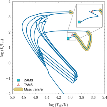
Figure 1. Evolution in the Hertzsprung-Russell (HR) diagram for a  star transferring mass to a
  point mass, assuming a mass transfer efficiency of
  . Symbols are shown at zero-age main sequence (ZAMS) and terminal-age main sequence (TAMS), together with parts of the track where RLOF is occurring. The inset shows evolution from ZAMS up to the beginning of the first phase of mass transfer.
Download figure:
Standard image High-resolution imageFigure 2 shows that MESAbinary computes the orbital evolution to a precision of a few parts in 104. We run this system using both the Ritter and the Kolb implicit schemes to display that under some circumstances the precise choice of mass transfer scheme does not play a big role in the evolution.

Figure 2. Evolution of mass transfer rate from a  to a
to a  point mass, assuming a mass transfer efficiency of
  . The upper panel shows the difference between the computed orbital separation and the analytical solution while the bottom one displays the evolution of the mass transfer rate, using two different schemes.
Download figure:
Standard image High-resolution image2.6.3. Spin–Orbit Coupling
We now test angular momentum conservation by ignoring all the mechanisms that remove angular momentum from the binary system. For this purpose we model an  binary with rotating components and an initial orbital period of 1.5 days. Due to the short orbital separation we assume the initial spin periods of the two stars are equal to the orbital period. The primary undergoes RLOF during the MS, initiating a phase of mass transfer on a thermal timescale. After transferring just
  the accretor also fills its Roche lobe, producing a contact system. At this point we terminate the evolution.
Figure 3 shows that spin angular momentum in both components increases during the pre-interaction phase, which is due to both stars expanding on the MS while remaining tidally locked. During RLOF, the secondary is rapidly spun-up, reaching nearly  of critical rotation before contact. The calculation of total angular momentum requires the summation of different contributions (orbital angular momentum and spin of both components). Therefore the maximum accuracy to which we can conserve angular momentum is limited by rounding errors. Figure 3 shows that conservation of angular momentum in the run is very close to machine precision.
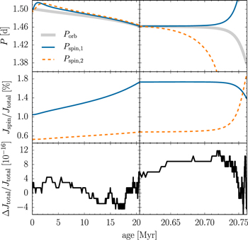
Figure 3. Angular momentum evolution in an  binary with an initial orbital period of 1.5 days. Left panels show the evolution before the onset of RLOF, while right panels display evolution from the beginning of RLOF until contact, when both components fill their Roche lobe. The fractional error in the total angular momentum is plotted in the bottom panel and is of order machine-precision.
Download figure:
Standard image High-resolution image2.6.4. Thermal Response to Mass Loss
The fate of binary systems depends largely on the precise value of  during an interaction phase, which depends on the thermal response of the donor star to mass loss. For WDs there is a limited range of accretion rates for stable hydrogen burning (Nomoto et al. 2007; Shen & Bildsten 2007). In MS binaries the evolution of the accretor radius depends on the mass transfer rate, and expansion during the interaction phase can lead to contact or even a merger (Wellstein et al. 2001).
We calculated an  binary system with an initial orbital period of 1.5 days using both MESAbinary and STARS. To minimize the modeling differences and focus on the thermal response of both components, we use an extremely simplified model that ignores internal mixing (including convective mixing). Under these conditions, the more massive star quickly depletes its central hydrogen and begins shell hydrogen burning, reaching RLOF and undergoing a phase of mass transfer on the thermal timescale. The resulting mass transfer rates are shown in Figure 4. The agreement is very good, despite mass transfer rates being computed in slightly different ways. Masses at detachment show a small difference, with the MESAbinary model terminating mass transfer when
  while the STARS calculation when
  . The figure also shows the change in radius of the accreting star, with two prominent peaks at
 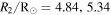 for MESAbinary and
  for STARS. The larger radius of the MESAbinary model is likely associated to the slightly higher mass transfer rates.
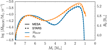
Figure 4. Mass transfer rate and accretor radius as computed by MESA and STARS for an  binary with an initial orbital period of 3 days. All internal mixing processes (including convective mixing) are turned off in the calculations.
Download figure:
Standard image High-resolution image2.7. Period Gap of Cataclysmic Variables (CVs)
Although CVs span a wide range of periods, observations show a lack of systems in the range  (see, for instance, Gänsicke et al. 2009). Such a feature is commonly explained by having an angular momentum loss mechanism "turn off" or become inefficient at some point. The most popular model for such a mechanism is magnetic braking (Rappaport et al. 1983), as the magnetic field of the donor is assumed to change quickly when the star loses enough mass to become fully convective.
We now compare to the results of Howell et al. (2001), who performed a population synthesis study to explore in detail the standard scenario involving magnetic braking. In Figure 5 we show the evolution of mass transfer rates and orbital periods for a set of CV models with different component masses and orbital periods. We run all models using  and
and  and magnetic braking is turned off when the donor star becomes fully convective. As an example the system with a
  donor (left panel in Figure 5) experiences a first phase of mass transfer induced by magnetic braking between
  and
and  , a non-interacting phase (the gap) between
  and
and  , and a subsequent phase of mass transfer dominated by gravitational wave radiation, reaching a minimum orbital period of about 1 hr at
  . As a comparison, for the same model Howell et al. (2001) obtain a first phase of mass transfer between
  and
and  , the gap occurs between
  and
and  and a period minimum is reached at
  . Figure 5 shows that our CV models spend most time away from the observed period gap.

Figure 5. Evolution of CV models under the effect of magnetic braking and gravitational wave radiation. For each track the label gives the donor mass, the WD mass, and the initial orbital period respectively. The gray band shows the observed period gap for CVs. These results reproduce Figure 1 in Howell et al. (2001).
Download figure:
Standard image High-resolution image2.8. Evolution of Massive Binaries
In massive stars, binary interactions have dramatic effects on the evolution of both components. Kippenhahn & Weigert (1967) introduced the term "case A" to refer to a mass transfer phase occurring in systems tight enough such that RLOF starts during the MS. This results in a large amount of mass being transferred on a thermal timescale, followed by a phase of mass transfer that proceeds on the nuclear timescale until the end of core H-burning. An additional phase of thermal-timescale mass transfer then follows (the so-called "case AB"), which strips the donor and produces an almost-naked helium star.
Here we show that MESAbinary can calculate the evolution of massive interacting binaries. We reproduce one of the models from Wellstein et al. (2001), a  system with an initial period of 3 days, using the same semiconvection efficiency of
  . As shown in Figures 6 and 7 this system experiences case A and AB mass transfer, and the accretor becomes a blue supergiant after core hydrogen depletion. The accretor depletes carbon before its donor.
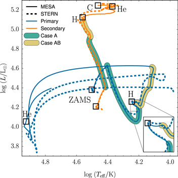
Figure 6. Evolution of a  system with a 3 day initial orbital period. MESAbinary models are compared to the results of Wellstein et al. (2001), which were calculated using the STERN code. The terms primary and secondary are used throughout the evolution to describe the initially more massive and the less massive components, respectively. For each component in the MESAbinary model, squares mark the ZAMS and the depletion of the indicated nuclear fuel in the core.
Download figure:
Standard image High-resolution image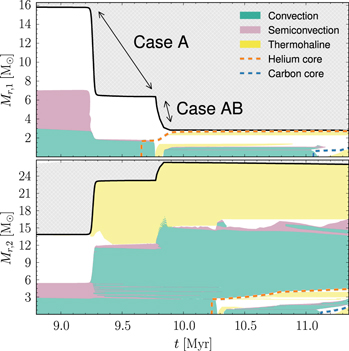
Figure 7. Kippenhahn diagram for the evolution of a  system with a 3 day initial orbital period. Most of the pre-interaction phase is not shown in this figure. The upper plot shows the evolution of the donor, while the lower plot displays that of the accretor.
Download figure:
Standard image High-resolution imageFigure 7 illustrates the prevalence of both thermohaline mixing and semiconvection in the accreting star. Newly accreted material is efficiently mixed inwards by thermohaline mixing. On the other hand the μ-gradient formed before interaction prevents the convective core from growing, with the efficiency of semiconvection controlling whether or not the star rejuvenates. Due to the choice of inefficient semiconvection, the core remains small, preventing the star from becoming a red supergiant. The star accretes a large amount of CNO-processed and helium-rich material. After being mixed through the envelope this material results in the surface being nitrogen rich and carbon depleted, with a slight enhancement in helium.
2.9. Rotating Binaries and the Efficiency of Mass Transfer
The efficiency of mass transfer plays a key role in close binary systems, but the processes by which material is lost from the system are not well-understood. In particular, whenever an accreting star approaches  , it is uncertain whether accretion can continue, one option being the development of a strong wind that prevents accretion (e.g., Petrovic et al. 2005; Cantiello et al. 2007). Whenever
  approaches one, we use an implicit method to iteratively reduce
  until this ratio falls below a threshold.
Tides counteract the effect of spin-up from accretion. Whether or not an accreting object reaches critical rotation depends on the efficiency of tidal coupling. Here we model a  binary system including differential stellar rotation, with an initial orbital period of 3 days and assuming initial orbital synchronization. Langer et al. (2003) argue that turbulent processes in the radiative envelope can significantly enhance tidal strength. They model the same system using the simple estimate for the synchronization timescale for a star with a convective envelope given by Zahn (1977),
  . For our implicit modeling of stellar winds we use a threshold of
  .
.
Figure 8 shows that MESAbinary models using both the Zahn (1977) and Hurley et al. (2002) timescales for tidal coupling. These models experience highly non-conservative phases of mass transfer, corresponding to the accreting star evolving very close to critical rotation. In particular during case AB mass transfer the accretor needs to switch from mass accretion to mass loss in order to remain sub-critical. As expected, the system with the tidal timescale from Zahn (1977) has a significantly higher mass transfer efficiency, and during the first phase of RLOF it only experiences a brief period in which the accretor reaches critical rotation. This is in broad agreement with the model by Langer et al. (2003).

Figure 8. Efficiency of mass transfer in a  binary system including differential rotation. The system is modeled with tides as described by Hurley et al. (2002) for radiative envelopes, and also with the simple tidal timescale given by Zahn (1977). The upper panel shows the efficiency of mass transfer, the middle panel the angular frequency of each star in terms of its critical value, while the lower panel shows the evolution of
  for both components.
Download figure:
Standard image High-resolution image2.10. Description of a Binary Run
MESAbinary performs each evolution step by independently solving the structure of each component and the orbital parameters, using the same timestep  for each. This approach differs from STARS, which simultaneously solves for the structure of both stars and the orbit in a single Newton–Raphson solver. Our choice to solve for each star separately gives a significant amount of flexibility and simplicity, as the examples in this paper demonstrate.
The top-level algorithm for evolving a star is described in Appendix B1 of Paper II. We modified this algorithm to support the new implementation of binary interactions, which is described in detail in the MESA documentation. Additional timestep limits are imposed in MESAbinary that consider relative changes between the radius and Roche lobe radius of both components, the total orbital angular momentum, the orbital separation, and the envelope mass in the donor.
3. PULSATIONS
The study of stellar pulsations (also termed oscillations) offers unique insights into the interiors of stars (Aerts et al. 2010). In some classes of star (e.g., solar-type, red giant), the stochastic excitation of hundreds of oscillation modes, typically by convective motions, allows remarkably detailed measurements to be made of the interior, including nuclear burning state (Bedding et al. 2011) and internal rotation (Beck et al. 2012). In other classes (e.g., classical Cepheid, β Cephei, δ Scuti, and γ Doradus pulsators), modes are instead excited by linear instabilities, most often linked to opacity variations in the envelope (the κ mechanism). In these latter objects, typically too few modes are excited for detailed asteroseismic analysis to be feasible; nevertheless, mapping out the regions of the theoretical HR diagram where the instabilities are expected to operate, and then comparing these instability strips against observational surveys, can often lead to new science.
Paper II introduced the astero extension to MESAstar, which permits on-the-fly refinement of stellar model parameters in order to fit a set of observed oscillation frequencies and spectroscopic constraints. Subsequent improvements to the astero capabilities include frequency correction recipes from Ball & Gizon (2014); implementation of the downhill simplex (Nelder & Mead 1965) and NEWYUO (Powell 2004) algorithms for  minimization; parameter optimization using only spectroscopic constraints (e.g.,
  and surface gravity); and coupling to the GYRE oscillation code, as an alternative to the ADIPLS code (Christensen-Dalsgaard 2008) used in the original implementation.
GYRE calculates the normal-mode eigenfrequencies  of a stellar model by solving the system of linearized equations and boundary conditions governing small periodic perturbations (
![$\propto \mathrm{exp}[i\sigma t]$](https://content.cld.iop.org/journals/0067-0049/220/1/15/revision1/apjs519320ieqn205.gif) ) to the equilibrium state. It is based on a novel Magnus Multiple Shooting (MMS) numerical scheme which is robust and accurate, and makes full use of all available processors on multicore computer architectures. The MMS scheme and the initial release of the code, which focuses on adiabatic pulsations, is described in Townsend & Teitler (2013); extensions to the code to support non-adiabatic pulsations are described in J. Goldstein & R. H. D. Townsend (2015, in preparation).
) to the equilibrium state. It is based on a novel Magnus Multiple Shooting (MMS) numerical scheme which is robust and accurate, and makes full use of all available processors on multicore computer architectures. The MMS scheme and the initial release of the code, which focuses on adiabatic pulsations, is described in Townsend & Teitler (2013); extensions to the code to support non-adiabatic pulsations are described in J. Goldstein & R. H. D. Townsend (2015, in preparation).
MESAstar couples to GYRE via two mechanisms. Loose coupling is achieved simply by MESAstar writing models out to disk, and GYRE subsequently reading these models in; we use this process below to map out massive-star instability strips. Tight coupling removes the intermediate disk usage, by handling all communication between MESAstar and GYRE in-memory; this permits fully closed-loop calculations, where the changes in the oscillation eigenfrequencies of an evolving stellar model are used to guide the further evolution of the model. Tight coupling allows GYRE to function as an alternative to ADIPLS in the astero extension, and opens up the possibility of other kinds of novel calculations, such as the automated location of instability-strip boundaries.
3.1. Massive-star Instability Strips
As an illustration of a large-scale calculation using MESAstar and GYRE loosely coupled, Figure 9 plots the instability strips for massive stars on and near the upper MS, for oscillation modes with harmonic degrees  . These strips are based on a set of 182 evolutionary tracks, each extending from the ZAMS across to a red limit at
  , with 101 tracks spanning the initial mass range
  in uniform logarithmic increments, and the remaining 81 tracks spanning the mass range
  in uniform linear increments (the latter set is designed to adequately resolve the "fingers" discussed below). OPAL opacity tables are used with the proto-solar abundances from Asplund et al. (2009), and for simplicity we neglect any rotation or mass loss. Convection is modeled with a mixing-length parameter
  = 1.5 and an exponential overshoot parameter
  , and the Schwarzschild stability criterion is assumed.
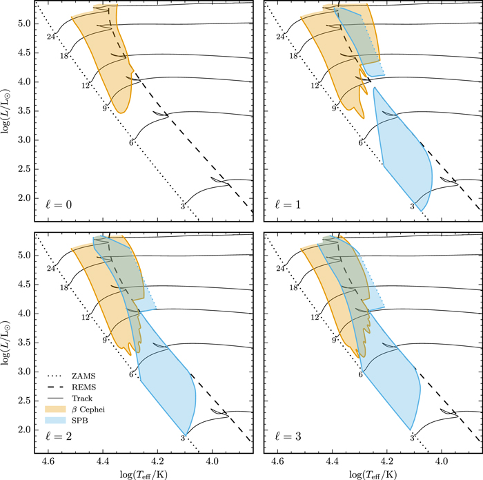
Figure 9. Instability strips for  oscillation modes in the upper part of HR diagram. Separate strips are shown for the β Cephei (
 1) and slowly pulsating B-type (SPB;
  1) classes of pulsating stars. The ZAMS and red edge of the main sequence (REMS) are shown for reference, as are evolutionary tracks for models with selected masses (labeled in solar units along the ZAMS). The red edges of the post-MS SPB strips are drawn with a dotted line, indicating that the positioning of these edges is an artifact of our numerical procedure.
Download figure:
Standard image High-resolution imageWe select points  along each of the 182 tracks (where i is the timestep index; see Section 6.4 of Paper I), chosen so that
  corresponds to the ZAMS,

across the  pair, and similarly for subsequent pairs. Here,
  and
and  are dimensionless weights which control the spacing of points in effective temperature and luminosity; we adopt the values 0.004 and 0.011, respectively, for these weights. At the selected points, GYRE searches for unstable oscillation modes with the harmonic degrees considered. First, GYRE solves the adiabatic oscillation equations to find eigenfrequencies
  falling in the range extending from the asymptotic frequency of the gravity (g) mode with radial order n = 400, up to the asymptotic frequency of the pressure (p) mode with radial order n = 10. Each
  is then used as an initial guess in finding a corresponding eigenfrequency
  of the full non-adiabatic oscillation equations. The real and imaginary parts of
  give the linear frequency
  and the growth e-folding time
  of a mode:

If  is negative, the mode is damped.
Separate strips are shown in Figure 9 for regions exhibiting unstable modes with  and
and  , where

is the dimensionless eigenfrequency; these correspond, respectively, to the β Cephei and slowly pulsating B-type (SPB) classes of pulsating stars. In β Cephei stars during the MS phase, p and g modes with periods of a few hours and radial orders  are excited by a κ mechanism operating on the iron opacity bump situated in the outer envelope at
  (Cox et al. 1992; Dziembowski & Pamiatnykh 1993). In SPB stars during the MS phase, g modes with periods of a few days and radial orders
  are excited by the same mechanism (Dziembowski et al. 1993). For masses
  the strips for both classes of stars extend into the post-MS domain. During this phase, unstable modes couple with g modes trapped near the boundary of the inert helium core. In the case of the SPB stars this leads to very high overall radial orders,
  , and ultimately limits our ability to follow the instability strips all the way to the red edge (our calculations are restricted to
  for computational efficiency reasons). Hence, in Figure 9 we plot the red edges of the post-MS SPB strips with dotted lines, to highlight that these are not the true red edges.
Allowing for differences in adopted abundances and other modeling parameters, the instability strips plotted in Figure 9 are in general agreement with those published in the literature (e.g., Pamyatnykh 1999; Zdravkov & Pamyatnykh 2008; Saio 2011). The notable difference is the presence of fingers in the lower boundaries of our β Cephei strips for  . Their appearance here is due to the unprecedented resolution in HR-diagram space of our stability calculations. To elucidate their origin, Figure 10 plots part of the
  frequency spectrum of an
  stellar model as it evolves from the ZAMS to the red edge of the main sequence (REMS), showing which modes are stable and which are unstable. The p1 mode is unstable over the effective temperature range
  , and the g1 mode over the cooler but overlapping range
  . The star then passes through a phase with no unstable modes, before the instability reappears in the range
  for the g2 mode.

Figure 10. The  = 1 dimensionless frequency spectrum of an 8.5
  stellar model as it evolves from the ZAMS to the REMS. Blue (orange) dots indicate which modes are stable (unstable); selected modes are labeled along the left/bottom edge using their classification.
Download figure:
Standard image High-resolution imageThis alternation between instability and stability, seen as fingers in Figure 9, stems from the fact that the κ mechanism only excites modes whose eigenfrequencies fall in a narrow range ![$[{\sigma }_{\mathrm{lo}},{\sigma }_{\mathrm{hi}}]$](https://content.cld.iop.org/journals/0067-0049/220/1/15/revision1/apjs519320ieqn243.gif) . At frequencies
. At frequencies  , the pulsation period becomes comparable to the local thermal timescale in the envelope region above the iron opacity peak, and this region behaves as a damping zone, stabilizing the modes. Conversely, at frequencies
  , modes couple with gravity waves trapped in the μ-gradient zone developing at the core boundary, and are likewise damped. The intermediate stable phase in Figure 10, between
  and
and  occurs when there are no modes in the
 ![$[{\sigma }_{\mathrm{lo}},{\sigma }_{\mathrm{hi}}]$](https://content.cld.iop.org/journals/0067-0049/220/1/15/revision1/apjs519320ieqn248.gif) range. As the star evolves, the unstable range narrows:
range. As the star evolves, the unstable range narrows:  decreases due to lower
  , while
  increases due to the growth of the μ-gradient zone.
Figure 11 shows a version of the  panel calculated using OP opacity tables rather than OPAL tables. There is an overall shift of the instability strips toward higher luminosities, an effect already noted by Pamyatnykh (1999). The fingers persist with much the same structure, supporting the fact that they are physical effects rather than numerical artifacts.

Figure 11. Instability strips for dipole ( ) oscillation modes in the upper part of the HR diagram, but calculated using OP rather than OPAL opacities (cf. Figure 9).
Download figure:
Standard image High-resolution imageReturning now to Figure 9, the post-MS extension of the SPB strips has been attributed in the literature to features in the Brunt–Väisälä frequency which reflect gravity waves at the boundary of the helium core, preventing them from penetrating into the core and being dissipated by strong radiative damping. Saio et al. (2006) and Godart et al. (2009) argue that the necessary feature is an intermediate convection zone (ICZ) associated with the hydrogen-burning shell, but more recently Daszyńska-Daszkiewicz et al. (2013) have shown that even a local minimum in the Brunt–Väisälä frequency is sufficient to reflect modes. In the present case, the empirical mass threshold  required for formation of an ICZ coincides with the lower boundaries of the SPB strip extensions. In the lowest-mass models above this threshold, the ICZ vanishes shortly after its appearance, but it leaves behind a narrow region with a steep molecular weight gradient. This gradient causes a spike in the Brunt–Väisälä frequency, which serves in a similar manner to prevent gravity waves from entering into the core and being dissipated.
The corresponding post-MS extension of the β Cephei strips was first noted by Dziembowski & Pamiatnykh (1993), but has not received much attention in the literature. Figure 9 shows that this extension has a well defined lower boundary, much like the SPB stars although situated at slightly higher masses,  . We have determined that the extension is also a consequence of ICZ formation; the shift to higher masses arises because it appears that multiple convection zones, rather than a single one, are necessary to reflect waves at the core boundary in the case of β Cephei pulsators.
3.2. Asteroseismic Optimization
To illustrate the updated asteroseismic capabilities of MESA, Figure 12 plots the echelle diagram for the subgiant star HD 49385, showing both the frequencies of  modes measured by Deheuvels et al. (2010), and the corresponding frequencies of the best-fit model determined using the astero extension. The calculations follow the same procedure detailed in Section 3.2 of Paper II; the only significant differences are that the initial mass, helium abundance, metal abundance and mixing length parameter are refined using the downhill simplex algorithm rather than the Hooke–Jeeves algorithm; oscillation frequencies are calculated using GYRE rather than ADIPLS; and the surface corrections to frequencies are evaluated using Equation (4) of Ball & Gizon (2014) rather than with the Kjeldsen et al. (2008) scheme.
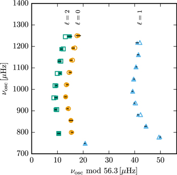
Figure 12. Echelle diagram for the subgiant star HD 49385. Observed frequencies are shown as filled circles ( ), triangles (
 = 1) and squares (
 = 2); black horizontal lines indicate the 1σ error bars. Calculated frequencies of the best-fit model are overplotted as the corresponding open symbols.
Download figure:
Standard image High-resolution imageComparing Figure 12 against Figure 8 of Paper II reveals only small differences between the two. The  of the best-fit models reported by astero is 2.3 in the former case, compared to 2.4 in the latter (cf. Table 2 of Paper II).
3.3. Automated Strip Location
The instability strips presented above involved the examination of ∼11 million modes of ∼40,000 stellar models. To partially automate the process, we can leverage tight coupling between GYRE and MESAstar. This is achieved by making small modifications to the extras_check_model callback routine in MESAstar (see Appendix B.1 of Paper II), so that GYRE is run after each timestep to determine the set of eigenfrequencies  of a user-specified group of modes. When
  changes sign from one timestep to the next for any of these modes, indicating that an instability-strip boundary has been crossed, a search is performed to find
  (
( )
)  0.
0.
Figure 13 presents an application of the tight coupling to the fundamental and first-overtone radial modes of the 8.5  model considered in Section 3.1, showing how the growth timescales
  and oscillation periods
  = 1/
= 1/ of the modes change as the star evolves from the ZAMS into the post-MS. The second-overtone radial mode remains stable,
  , over the range plotted. The vertical lines show where
  changes sign. The blue and red edges of the (
 ) β Cephei instability strip can be seen in the upper panel of Figure 13 at
  and
and  , respectively. The blue edge12
of the classical instability strip can likewise be seen in both panels at
, respectively. The blue edge12
of the classical instability strip can likewise be seen in both panels at  . The corresponding red edge is not found because GYRE does not include a treatment of the pulsation–convection interaction—a necessary ingredient for modeling the classical red edge (see, e.g., Section 3.7.3 of Aerts et al. 2010, and references therein).
Figure 13. Growth timescale  (left axis) and oscillation period
  (right axis) of the fundamental and first-overtone radial modes of a 8.5
  model, plotted as a function of
  as the star evolves away from the ZAMS. The vertical dashed lines, determined automatically, show the points where the modes switch from stable (
 ) to unstable (
 ), and vice versa.
Download figure:
Standard image High-resolution imageAs a further demonstration of automated instability strip location, Figure 14 plots the blue edges of the classical instability strip in the HR diagram, for fundamental and first-overtone radial modes. The edges are calculated for 51 evolutionary tracks spanning the initial mass range  in uniform logarithmic increments. At luminosities
  corresponding to classical Cepheid pulsators, these edges show good agreement with the set B results published by Smolec & Moskalik (2008, their Figure 1). At luminosities
  corresponding to δ Scuti stars, the edges are somewhat cooler than results published in the literature; however, this is because we consider only fundamental and first-overtone modes, whereas the blue edge is typically set by higher overtones which are displaced toward hotter
  (e.g., Dupret et al. 2004, their Figure 1).

Figure 14. Calculated blue edge of the classical instability strip, for fundamental and first-overtone radial modes. The corresponding dashed lines show the predictions from set B of Smolec & Moskalik (2008, their Figure 1).
Download figure:
Standard image High-resolution imageIdeally, the same automated approach could be used to locate the boundaries of the non-radial ( ) instability strips plotted in Figure 9. In practice it is very challenging to devise a robust algorithm that can unambiguously interpret the eigenfrequencies produced by GYRE. Sometimes, acoustic glitches in a model can trap modes in surface layers, where they are strongly excited; however, these modes are very sensitive to model parameters, and it is unclear whether they are physically meaningful or not.
4. IMPLICIT HYDRODYNAMICS
Shocks happen in stars, such as after a massive star collapses, or cyclically in the outer envelopes of stars pulsating at sufficiently large amplitude. Previous versions of  allowed large velocities such as those encountered in the last few seconds leading to a core collapse (
 ), but there was no provision for large jumps in velocities leading to shocks. In this section we describe the changes that have been made to support an implicit treatment of hydrodynamic shocks that includes careful attention to conservation of energy. We demonstrate that the revised equations are intrinsically conservative in the sense that deviations from exact energy balance can only arise from residual numerical errors in the approximate solutions rather than from the form of the equations themselves. Following the description of the changes, we show a series of envelope shocks as a test of the implementation. The form of the equations and the demonstration of intrinsic conservation closely follow Fraley (1968) and Grott et al. (2005). The treatment of artificial viscosity is based on Weaver et al. (1978).
4.1. Mass Continuity
The specific volume of cell k is

where rk is the outer face radius,  is the inner face radius,
  is the cell mass, and
  is the cell average density (see Figure 15 for the layout of cells in MESAstar).We create an initial algebraic form of the continuity differential equation by dividing the change in the specific volume in a step by the length of time
  , using step start and end values for rk,
  , and
, and  and the value
  which is constant during the step:
Next, we rewrite the right-hand side introducing variables for the time centered velocity  and the effective area A to get the final form of the mass continuity equation as used in
  :
:

where

and rk is evaluated as

Algebraic simplification then shows that

To be consistent with the mass continuity equation, we use these expressions for effective area and time centered velocity in the following momentum and energy equations. It will be shown below that to get intrinsic energy conservation, we must time center the velocity and use special combinations of starting and ending radius in a couple of places, but all other terms in the equations can remain fully implicit to avoid degrading the numerical stability as would happen in a uniformly time-centered scheme.
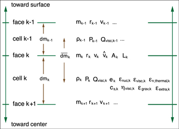
Figure 15. Schematic of relevant cell and face variables relevant for hydrodynamics in  .
.
Download figure:
Standard image High-resolution image4.2. Artificial Viscosity
In  , the artificial dynamic viscosity coefficient
  (which has the dimensions
  )
)

where the linear term is

and the quadratic term is

with 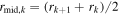 ,
,  the sound speed in cell k, and l1 (l2) is a dimensionless coefficient for the linear (quadratic) term. The linear term is rarely used; it provides for a general damping of pulsations. The quadratic term is only nonzero in regions of compression and is the primary control for the strength of artificial viscosity. Assuming the usual case of l1 = 0, the shock front is spread over a distance
  . We follow Dorfi (1998) in opting for a shock spread proportional to the local radius r rather than the local cell width. This choice is dictated by the fact that step-by-step adjustments to the mesh resolution lead to dynamically changing, non-monotonic variations in cell widths of up to a factor of 2 or more between neighboring cells. Making the shock spread directly dependent on the local cell widths would produce numerically intolerable dynamically changing, non-monotonic variations in cell-to-cell values for the shock spread. Use of a local running average cell width is also ruled out by the need to keep algebraic equations dependent only on nearest neighbors to allow a block tridiagonal matrix solution. The use of a small fraction of the local radius gives a smoothly varying shock spread that avoids the numerical problems associated with using the cell width.
We define the quantity  (having dimensions of energy), in cell k as

The momentum equation uses  in an expression that defines an artificial acceleration analogous to the pressure gradient term, and the energy equation uses it to define an artificial viscous heating analogous to the mechanical work term.
4.3. Specific Linear Momentum Equation
The local linear momentum conservation equation at face k between inner cell k and outer cell  is
is

where 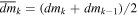 is the mass associated with face k, and the viscous acceleration term at face k is

The use of the product  in the denominator of the gravitation term is necessary for intrinsic energy conservation as will be shown below.
4.4. Specific Energy Equation
The local energy conservation equation for cell k between outer face k and inner face  is
is

where ek is the specific thermal energy for cell k. The viscous heating rate for cell k is

Energy loss from weak reaction neutrinos is already subtracted from the nuclear burning term,  , so only the neutrino energy loss rate from thermal processes,
  , is explicitly accounted for in Equation (37). An example of
  is the artificial injection of energy to trigger a shock.
An alternative form of the energy equation equates the model  to the expected value

where

and

Using Equation (27), the expression for  can be rewritten

thereby avoiding the use of velocities and thus be appropriate for hydrostatic cases.
4.5. Intrinsic Energy Conservation
The summed kinetic, potential, internal energies are


and thus the total energy of the star is  . We now explicitly demonstrate that the equations we solve are formulated in such a way that the rate of change of total energy exactly equals the combined energy sources and sinks.
Multiplying Equation (35) by  gives an equation with units of luminosity:

Using Equation (29) to eliminate  in the first term on the right,

shows that this term is the negative of the rate of change of potential energy, a result that is made possible by the use of the  in Equation (35) instead of an alternative such as
  . Thus, Equation (46) can be written as
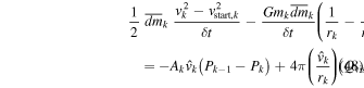
Similarly, multiplying Equation (37) by  also yields an equation with units of luminosity:

Adding Equations (48) and (49) and summing over the grid index k gives
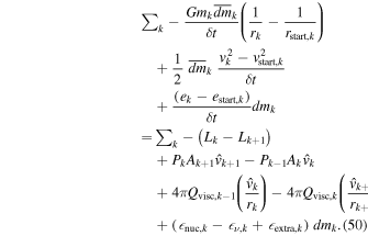
The sum over the pressure terms is
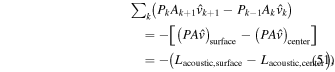
which cancels term by term except at the boundaries. We define  as the work done by the model on the atmosphere at the surface and
  as the work done on the model at the center, for example, by an artificial piston. The sum over the artificial viscosity terms leads to a similar expression, but because Qvisc vanishes at the surface and the center, the sum equals zero. That is, the energy added by artificial viscous heating in the energy equation exactly balances the loss of kinetic energy by artificial viscous acceleration in the momentum equation.
The terms on the left-hand side of Equation (50) are the difference in the total energy between the start and end of a step divided by the length of the step, in other words, the average rate of change of the total energy of the model. Therefore Equation (50) can be written as

This equation embodies conservation of energy in  : the rate of change of total energy equals the combined energy sources and sinks. This demonstrates that in the given form, the algebraic equations intrinsically conserve energy in the sense that failure to get energy balance can only arise from the residual numerical errors that are inherent in using approximate solutions to the equations. This in turn means that to control energy balance errors, we can focus on reducing residuals either by changes in the Newton solver or by timestep reductions.
4.6. Controlling the Accuracy of Energy Conservation
The Newton solver considers both the sizes of incremental changes to the variables and the sizes of residual errors for the equations. For the energy equation, the residual used by the solver is defined to be the timestep  times the difference between the left and right sides of Equation (37) divided by
  ; in other words, the residual is the error as a fraction of the specific energy at the start of the step. By adjusting tolerances for the average and maximum size of residuals, we force the Newton solver to take extra iterations to reduce the residuals which will in turn reduce the total error in energy conservation.
A second and related way to control energy conservation errors is to use the average and maximum energy residuals to adjust the timesteps. For example, if the maximum magnitude for an energy residual exceeds a specified hard limit, then the proposed solution is rejected and the step is retried with a smaller timestep. If the maximum is smaller than the hard limit but exceeds another specified limit, then there is no forced retry for this step, but the next timestep is reduced by the ratio of the limit divided by the maximum magnitude. If the maximum is smaller than both limits, then other factors determine the next timestep. Later in this section, we will show that these approaches in combination with the intrinsic conservation form of the equations yield a solution for a shock in an envelope that evolves with reasonably large timesteps while conserving energy to a high degree of accuracy.
4.7. Limiting Acceleration of Convective Velocity
When using hydrodynamics, we often require timesteps that are so small that we need to limit the increase in convective velocities as calculated in the standard instantaneous mixing length theory (MLT) so that they do not assume unphysically large accelerations. If convection velocities are allowed to adjust instantaneously, then our methods for artificially creating shocks will fail since however rapidly we inject energy over a limited region, convection will be able to transport the energy away. To be able to simulate shocks we need to have a way to limit convection velocity acceleration.
The primary scheme we use for this is derived from Arnett (1969) and Wood (1974). The MLT implementation in MESA has been extended to take as additional arguments the timestep and the previous convection velocity at the same mass location ( ). It calculates a provisional convection velocity (
 ) using the standard instantaneous MLT, then defines a convective timescale (
 ) as the local pressure scale height (H) divided by the sum of the provisional plus previous velocities. If
  is less than
  , then the next convection velocity (vc) is only incremented from the previous one by the difference of the provisional minus the previous velocities times the ratio of the timestep divided by the timescale

where

As an alternative scheme for limiting convection acceleration, we also allow the maximum rate of change of convection velocity to be set as a fraction,  , of the local gravitational acceleration. If
  , then

The final vc is used to recalculate the convection efficiency, which is used to calculate the MLT temperature gradient.
These methods for limiting the acceleration of convective velocities reduce the energy transport rate as well as the rate of compositional mixing. Both schemes seem to give at least qualitatively reasonable results and avoid the problems of unphysically large accelerations that are possible with standard instantaneous MLT. Hopefully this ad hoc solution will soon be replaced by a quantitatively correct formulation.
4.8. Surface Boundary Conditions
MESA provides a variety of options for surface boundary conditions (see, e.g., Section 5.3 of Paper I), and several more have been added for use with hydrodynamics. The simplest allow specification of a particular value for the surface pressure, the surface temperature, or the  if the surface is not at the photosphere. In the case of a given fixed surface pressure, the corresponding surface temperature is set using the surface luminosity and radius based on the usual blackbody relation. For the second case, where the surface temperature is fixed, the surface pressure is set to the corresponding radiation pressure. For both of these, if the surface is not at the photosphere,
  is set using the Eddington T–τ relation. Finally, for specified
  when the surface is not at the photosphere, the corresponding surface temperature is also derived using the Eddington T–τ relation, and the surface pressure is set to the radiation pressure for that temperature.
For computations involving shocks at the surface, there is an option to use boundary conditions that specify a vanishing gradient for compression at the surface and a temperature corresponding to blackbody radiation. The outermost cells ( ) satisfy the equation

which represents the vanishing of the surface compression gradient.
Finally, for computations involving interior shocks but low velocities at the surface, there is an option to use the surface pressure from the selected atmosphere prescription with the momentum equation relating the surface velocity to the surface pressure gradient. This form for the surface boundary conditions is used in the shocked massive star example in Section 6 and in the following envelope shock test.
4.9. Shock Test
To test the implementation, we shock the extended envelope of a 6.93  asymptotic giant branch (AGB) star evolved from a 7
  MS star without rotation and an initial metallicity of 0.001. This case is chosen because of the uniform properties of the extended envelope (i.e., small density range, smooth density, and uniform composition). Our interest is to study the propagation of the shock, the properties of the shocked material, and the magnitude of energy conservation errors. In Section 6, we present results that mimic core-collapse supernovae.
Explosion simulations with MESA start from a converged model. The core is excised by removing inner shells of the model and setting new inner boundary conditions for mass, radius, velocity, and luminosity. For the current test, we remove the center just above the helium core at a mass of 2.40  which corresponds to an inner radius of 27.2
  . The stellar surface lies at a radius of 282.7
  . During the following evolution, the excised region is treated as a point mass and is linked to the above layers by the inner boundary conditions which can be changed at each timestep to simulate various core events. The model grid was adjusted at each step to give higher resolution in the vicinity of the shock. The total number of cells stayed at about 1000, with cell masses dropping to about
  of the total in approximately 100 cells around the shock.
In MESA, the artificial explosion that creates a shock can be produced in three ways: a piston, a luminosity flash, or a thermal bomb.
- 1.The first option changes the inner boundary conditions for velocity and radius to mimic a piston. A core-collapse supernova can be simulated by moving the inner radius inwards (collapse) at a free-fall speed and then violently outwards (bounce and explosion). The parameterization for the piston-driven explosion is the same as that described in Woosley & Weaver (1995), and includes the infall piston time, the final inward piston radius, the initial outward piston speed, and the final piston radius.
- 2.The second option increases the inner boundary luminosity over a specified time in order to deliver the desired total energy. In this approach, the inner boundary radius is fixed at all times and becomes a zero-flux inner boundary once the flash is over. In this approach, the inner boundary radius is fixed (zero velocity) and we inject the energy within the first zone of the domain.
- 3.The third option deposits energy at a constant rate during a specified time and in a region bounded by two specified Lagrangian-mass coordinates. As in the second option, the inner boundary radius is fixed at all times.
The differences among these three options can alter the properties of the shocked envelope.
To benchmark MESA for these shock tests, we have used the explicit radiation-hydrodynamics code V1D (Livne 1993; Dessart et al. 2010a, 2010b). Options 1 and 3 are implemented in V1D. For the present envelope shock test, and subsequently for the explosion tests, we use option 3 in both codes. We initiate the explosion by depositing a total of 1049 erg at a constant rate over 10 s between the Lagrangian mass coordinates of 2.40 and 2.45  . This energy deposited is well in excess of the initial binding energy, which is approximately
  1047 erg. Once the energy injection is over, we save a model which is then used as initial conditions for a shock evolution simulation.
Once the stellar core has been excised, the remaining envelope has a smooth density profile, resembling a power law whose exponent is −1 at depth and decreases outwards to become about −10 at the photosphere (top row panels of Figure 16). Because convective accelerations are limited, the energy deposited increases the internal energy within the innermost 0.05  of the grid. The pressure build-up leads to the sudden expansion of the innermost layers and the formation of a mildly supersonic shock (Mach number
  ). The shock propagates at a velocity in excess of 1000
  initially, but slows to a few 100
  by the time it reaches the stellar surface after 3 × 10⁵ s. The density contrast across this somewhat weak shock is
  . For a strong shock, one expects a density jump of 4 for an ideal gas with an adiabatic index of 5/3 and a value of 7 for a radiation-dominated gas (
 4/3).
4/3).

Figure 16. Multi-epoch snapshots for the hydrodynamical simulation of a 1049 erg shock in the envelope of a  AGB star. We show the density (top row), temperature (middle row), and velocity (bottom row) vs. Lagrangian mass (left column) and radius (right column). In each panel, the solid line refers to the MESA results and the dashed line to the V1D results.
Download figure:
Standard image High-resolution imageThis simulation is analogous to a shock-tube test. However, in the stellar context (realistic stellar envelope, realistic equation of state, spherical expansion), there is no analytical solution for comparison. We thus run the same simulation with the code V1D and include the results in Figure 16. The results agree at multiple times spanning the progression of the shock toward the stellar surface (the times used for comparison are the same to within 1% and the grid resolution is comparable). The sharpness of the shock in the two simulations differs with time and location. In V1D, the artificial viscosity has a physical spread of two grid zones, irrespective of radius, while in this MESA run, the spread is set to 0.1% of the local radius (see Section 4.2).
Since the explosion is started as a thermal bomb, the bulk of the energy is initially internal (see Figure 17). As the material expands and accelerates, the kinetic energy increases, mirroring the decrease in internal energy (essentially no energy is used to unbind the envelope). At the time of shock emergence, the internal and kinetic energies are comparable.
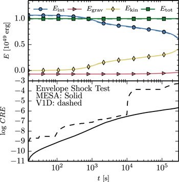
Figure 17. Top: evolution of internal energy  , gravitational energy
  , kinetic energy
  , and their sum
  for the envelope shock test simulated with MESA and V1D. Bottom: log of cumulative relative error CRE (Equation (58)) of the total energy
  . We neglect sources (nuclear burning) and sinks (radiation losses), which are negligible.
Download figure:
Standard image High-resolution imageIn the present case, we can preserve good accuracy while still allowing timesteps an order of magnitude greater than the Courant time.13 The error in energy conservation at timestep i is

where  is the right-hand side of Equation (52) multiplied by
  . The cumulative relative error in energy at a timestep n is

In the test case, after about 15,100 timesteps when the shock reaches 6.6  , the cumulative relative error has grown to about
  , corresponding to a roughly linear growth rate of about
  per step (bottom panel in Figure 17). Note that at this stage of evolution the shock is nearing the outer edge of the envelope but has not actually broken out through the surface. Issues of shock break out are beyond the scope of the current implementation. Using the parameters selected for the test, the energy conservation with V1D is not as good as with MESA (the jumps in cumulative error correspond to times when the limit on the timestep are loosened); comparable accuracy can be obtained with V1D by reducing the explicit timestep well below the Courant limit.
Finally, to illustrate the effects of artificial viscosity, we vary the quadratic term l2 that controls the spread of the shock in response to compression (see Equation (33)), with the explosion energy increased to 1050 erg in order to produce a stronger shock, and otherwise the same parameters and initial conditions. The top panel of Figure 18 shows the artificial acceleration ( ) and energy (
 ) terms that enter the momentum and the energy equations for
  0.001. The acceleration term is positive ahead of the shock, causing a pre-acceleration of the unshocked material, and negative behind the shock causing a deceleration of the post-shock material. The energy corresponding to those changes in momentum is balanced by the extra term for artificial viscous heating in the energy equation (
 ). The lower panel of Figure 18 shows the expected increase in the width of the shock as we raise the parameter l2. For the model with
  0.004, dots locate grid cells. Note that with the smallest value (
 0.001), the velocity is showing small oscillations ("ringing") behind the shock indicating that we have reached a practical lower bound for the shock spread given the other parameter choices and the nature of the specific problem.

Figure 18. Top: normalized values of velocity, artificial acceleration  , artificial viscous heating
  , and Mach number in the vicinity of the shock. The dashed vertical line marks where the Mach number is unity. Bottom: dependency of the shock morphology on changes in the viscosity parameter l2. The dots shown for the model with
  0.004 denote the location of the MESA grid points at that time. For all these tests, we deposit an energy of 1050 erg at a constant power over 1 s.
Download figure:
Standard image High-resolution image5. ADVANCED BURNING
For the advanced stages of stellar burning, we show here that more accurate summations yield more efficient time integrations. This development allows MESA to use large in situ reaction networks. It offers an improvement by providing a single solution methodology that avoids the challenges of stitching together different solution methods such as nuclear statistical equilibrium (NSE) or co-processing a reaction network. We discuss this development and apply it to the evolution of an X-ray burst on a neutron star (NS). In Section 6 we discuss the pre-supernova progenitors and combine the new capability for advanced burning with the implicit hydrodynamics module to discuss the explosion of core-collapse supernovae.
The equations that describe the continuum limit of reacting nuclei are

where Yi is the abundance of isotope i, λ is a reaction rate, and the three sums are over reactions which produce or destroy a nucleus of species i with 1, 2, and 3 reacting nuclei, respectively (e.g., Meyer et al. 1998; Hix & Meyer 2006; Guidry et al. 2013; Longland et al. 2014). The positive or negative stoichiometric coefficients ci account for the numbers of nuclei created or destroyed in a reaction. The factorials in the denominators avoid double counting of identical particles.
Figure 19 shows the evolution of the mass fractions for a MESA one-zone burn at constant T = 9.6 × 10⁹ K and ρ = 6.0 × 10⁹ g cm−3 for 106 s starting with a pure 28Si composition. The 204 isotope network, mesa_204.net, used in the calculation is listed in Table 2, and includes the isotopes identified in Heger et al. (2001) as important for  in core-collapse models. The thermonuclear reaction rates are from JINA reaclib version V2.0 2013-04-02 (Cyburt et al. 2010). Implementation of reaction rates and associated quantities are described in Paper I and Paper II.

Figure 19. Evolution of the composition for a one-zone burn at constant T = 9.6 × 10⁹ K and ρ = 6.0 × 10⁹ g cm−3 for 106 s starting with a pure 28Si composition. The calculation uses the mesa_204.net isotope listing (see Table 2), the most abundant isotopes are drawn with thick lines, and several isotopes are labeled. The initial composition is quickly erased as NSE for  0.5 is established by
  10−8 s. Several orders of magnitude in time pass before weak reactions drive a second period of rearrangement. By
  s a second NSE quiescent period with
  0.403 is established.
Download figure:
Standard image High-resolution imageTable 2. 204 Isotope Network Listing
| Element |

|

|
Element |

|

|
|---|---|---|---|---|---|
| n | ⋯ | ⋯ | S | 31 | 37 |
| H | 1 | 2 | Cl | 35 | 38 |
| He | 3 | 4 | Ar | 35 | 41 |
| Li | 6 | 7 | K | 39 | 44 |
| Be | 7 | 10 | Ca | 39 | 49 |
| B | 8 | 11 | Sc | 43 | 51 |
| C | 12 | 13 | Ti | 43 | 54 |
| N | 13 | 16 | V | 47 | 56 |
| O | 15 | 19 | Cr | 47 | 58 |
| F | 17 | 20 | Mn | 51 | 59 |
| Ne | 19 | 23 | Fe | 51 | 66 |
| Na | 21 | 24 | Co | 55 | 67 |
| Mg | 23 | 27 | Ni | 55 | 68 |
| Al | 25 | 28 | Cu | 59 | 66 |
| Si | 27 | 33 | Zn | 59 | 66 |
| P | 30 | 34 | ⋯ | ⋯ | ⋯ |
Download table as: ASCIITypeset image
The thermodynamic conditions used in Figure 19 are representative of the central regions of massive stars during the advanced stages of evolution. At such temperatures the initial composition of pure  undergoes a rapid readjustment. The timescale for the initial
 0.5 composition to relax to an NSE composition is roughly
  s =
s =  s (Khokhlov 1991; Calder et al. 2007), commensurate with the first burning phase in Figure 19. Between
  −8 s and
  10−4 s the isotopes 4He and 54Fe dominate the
 0.5 NSE composition. Since T and ρ are constant, only changes to
  can change the abundances. A second period of intense rearrangement begins at
  −4 s and ends at
  s. This activity is driven primarily by
  and
and  and other weak reactions that change
  . Beyond
  s, the isotopes 48Ca, 49Ca, and 51Sc dominate the
  NSE composition.
Table 3 shows the sensitivity of the final  in this calculation to the number of isotopes in the network. Each successively larger network encompasses the previous smaller network and was crafted to yield approximately the same final
  value as given by the largest network. The 204 isotope network used in Figure 19 is in the regime where larger networks give the same final
  to 3 significant figures.
Table 3.
Final  for Figure 19
| # of Isotopes |

|

|

|
|---|---|---|---|
| 75 | 0.4093 | Ni | 68 |
| 125 | 0.4065 | Ni | 68 |
| 160 | 0.4032 | Ni | 68 |
| 204 | 0.4032 | Zn | 66 |
| 368 | 0.4035 | Zn | 77 |
| 833 | 0.4029 | Sn | 125 |
| 3298 | 0.4039 | At | 211 |
Download table as: ASCIITypeset image
5.1. More Accurate Summations Yield More Efficient Integrations
We now test different summation methods for Equation (59) and demonstrate that improved accuracy of the summations reduces the number of timesteps with a commensurate reduction in the execution time—while producing the same answers to within the specified integration accuracy.
When the summations in Equation (59) are accumulated in IEEE 64-bit arithmetic (16 significant figures, real*8 precision in Fortran on most architectures; more specifically binary64 with round to nearest and round ties to even) the integration in Figure 19 takes 3062 timesteps using a variable-order Bader–Deuflhard integrator with a specified accuracy of  = 10−4 and a scaling value
  = 10−3. The specified accuracy
  limits the maximum error over one timestep for any isotope. Other potential, but less demanding, choices for the meaning of
  include limiting the average or root-mean-square error over one timestep for all isotopes. When an abundance is greater than
  a relative error is calculated, while for abundances smaller than
  , the absolute error is calculated (e.g., Press et al. 1992). In essence, only abundances greater than
  can exert control on the size of the timestep.
When the summations are accumulated in IEEE 128-bit arithmetic (32 significant figures, real*16 precision in Fortran on most architectures), the same integration takes only 55 timesteps, a factor  improvement in the number of timesteps, and a factor of
  less execution time. Both calculations returned the same answers to within the specified integration error tolerances. For tighter integration tolerances of
  = 10−6 and
  = 10−5, the evolution with summations in IEEE 64-bit arithmetic takes 10,081 timesteps while the evolution with summations in IEEE 128-bit arithmetic takes 88 timesteps. This is a factor of
  improvement in the number of timesteps, a factor of
  in execution time, with both calculations again producing the same abundances to within the specified integration error tolerances. Both sets of integration tolerances are practical, everyday usage tolerances; they are not extreme cases of hypothetical interest only. Using low-order Rosenbrock and first-order Euler integrators also showed similar improvements in the number of timesteps when the summations were performed in IEEE 128-bit arithmetic instead of IEEE 64-bit arithmetic. We achieve a reduction in the number of timesteps and execution times regardless of the number of isotopes, choice of integrator, integration tolerances, or linear algebra solver. This improvement in efficiency is fundamentally driven by a reduction in the numerical noise of the function being integrated.
At temperatures larger than ≈5 × 10⁹ K, integrating Equation (59) can be challenging as terms in the summation usually become large and opposite in sign. As shown above, the classic symptom during an integration under these thermodynamic conditions is the integrator taking an excessive number of very small timesteps in order to satisfy the specified integration accuracy criteria. The traditional workaround to this numerical problem is abandoning a network integration at elevated temperatures and deploying equilibrium solution methods. This switching of methods raises its own numerical issues when used within the larger context of multi-dimensional simulations or stellar evolution models (see Section 5.2).
Unless precautions are taken the summation of large sets of numbers can be very inaccurate due to the accumulation of rounding errors. Methods for accurate summation within the bounds of a given arithmetic remain an active field of research (e.g., Demmel & Hida 2003; McNamee 2004; Ogita et al. 2005; Rump et al. 2008; Graillat & Ménissier-Morain 2012; Collange et al. 2014). These summation discrepancies also worsen on heterogeneous architectures—such as clusters with NVIDIA GPUs or Xeon Phi accelerators—which combine programming environments that may obey various floating-point models and offer different precision results.
The summations in Equation (59) for the neutron, proton, and α-particle abundances are especially prone to inaccuracies because every isotope in a network reacts with these three particles. We report on the summation errors for these three isotopes. Each term in the summations of Equation (59) is calculated using IEEE 64-bit arithmetic and then copied into a IEEE 128-bit variable using the Fortran promotion rules. Each IEEE 128-bit term is then imported into the MP (Brent 1978) and MPf90 (Bailey 1995) multiple precision packages. All other aspects of the integration were executed in IEEE 64-bit arithmetic. The summations are then accumulated with
- 1.IEEE 64-bit: terms in the order as given;
- 2.IEEE 64-bit: terms sorted by their absolute value in ascending order;
- 3.IEEE 64-bit: terms sorted by their absolute value in ascending order and the Kahan (1965) algorithm, which reduces the numerical error in summation by retaining a separate variable to accumulate the errors;
- 4.IEEE 128-bit: terms in the order as given;
- 5.IEEE 128-bit: terms sorted by their absolute value in ascending order;
- 6.MP and MPf90 100 digits: terms sorted by their absolute value in ascending order.
There are many summation methods and alternative multiple precision packages we did not deploy in these studies (e.g., Knuth 1997; Higham 2002; Li et al. 2002; Muller et al. 2010; Collange et al. 2014).
Table 4 summarizes these summation experiments. We confirm that 100 digits are sufficient to prevent errors in our multiple precision sums. Column 4 gives the minimum number of correct digits in a summation. There are three time periods in the evolution of Figure 19 where summations performed in IEEE 64-bit arithmetic greatly increase the number of timesteps taken by the integration. One is during the first rearrangement into the NSE state ending around 10−8 s, another is during the second rearrangement around 10−1 s and the third time period is when the abundances do not change much ( 0) and reaction rates reach equilibrium. It is during these equilibrium periods where a summation in IEEE 64-bit arithmetic with the terms summed in the order given may yield only six accurate digits. As a result, 3062 timesteps are needed to complete the integration (e.g., row 2 of Table 4). It is important to note that this strategy and choice of arithmetic is commonly used by nuclear reaction networks (e.g., Timmes 1999)—and is the most inaccurate choice. Row 4 of Table 4 is an important case, sorted plus Kahan summation, because it demonstrates that a marginal improvement in the accuracy of the summation (8 minimum correct digits) has a major reduction on the number of timesteps (1174 timesteps) and execution time (a factor of
  smaller). This establishes the general trend that improved accuracy of the summations reduces the number of timesteps with a commensurate reduction in the execution time—while producing the same answers to within the specified integration accuracy.
Table 4. Results of Summation Experiments
| IEEE | Maximum | Strategy | Minimum | Number of | Ratio of |
|---|---|---|---|---|---|
| Arithmetic | Digits Compared | Correct Digitsa | Timestepsb | CPU Timesc | |
 = 10−4 = 10−4  = 10−3 = 10−3 |
|||||
| 64-bit | 16 | in order given | 6 | 3062 | 31.7 |
| 64-bit | 16 | sorted, ascending | 7 | 2614 | 24.4 |
| 64-bit | 16 | sorted, Kahan sum | 8 | 1141 | 13.1 |
| 128-bit | 32 | in order given | 21 | 55 | 1.0 |
| 128-bit | 32 | sorted, ascending | 22 | 55 | 1.0 |
 = 10−6 = 10−6  = 10−5 = 10−5 |
|||||
| 64-bit | 16 | in order given | 6 | 10081 | 156 |
| 64-bit | 16 | sorted, ascending | 7 | 7972 | 123 |
| 64-bit | 16 | sorted, Kahan sum | 8 | 7674 | 112 |
| 128-bit | 32 | in order given | 21 | 88 | 1.0 |
| 128-bit | 32 | sorted, ascending | 22 | 88 | 1.0 |
Notes.
aRelative to the 100 digit sum by the MP and MPf90 multiple precision packages. bFor a Bader–Deuflard integrator in IEEE 64-bit arithmetic. cFor a single thread on one 2.7 GHz Intel Xeon E5 core with the Intel 15.0.1 Fortran compiler, and relative to the execution time for the integration with 128-bit summations with terms in the order given.Download table as: ASCIITypeset image
The left-hand side of Equation (59) for  is a IEEE 64-bit array to be filled with one of the summations. Setting
  equal to one of the IEEE 128-bit summations (at least 22 digits of accuracy) or the multiple precision package summations gives the most efficient integration (55 timesteps, rows 5 and 6 in Table 4) because the Fortran precision demotion rules assure
  is accurate to the limit of IEEE 64-bit arithmetic. The next best strategy, but a distant second, is setting
  equal to the sorted, Kahan summation. The worst case is setting
  equal to the 64-bit arithmetic sum with the terms in the order they appear—which is a common approach (e.g., Timmes 1999).
Figure 20 shows the number of correct digits in 64-bit and 128-bit summations for  (4He) with the terms accumulated in the order they are given. The number of correct digits is measured against the 100 digit sum calculated by the multiple precision packages MP and MPf90. The choices for the integrator and integration tolerances are the same as in Figure 19. Figure 20 shows that the minimum number of accurate digits is usually within a few digits of the limit of IEEE 64-bit arithmetic, but degrades to 6 digits (see row 1 of Table 4) during a time period of intense isotope rearrangement. These relatively large inaccurate summations cause the right-hand side of Equation (59) to be poorly defined in IEEE 64-bit arithmetic. As a direct result, the integration of Equation (59) with IEEE 64-bit summations takes 3062 timesteps to complete. Sorting the terms in the sums in ascending order and using the Kahan summation algorithm results in an accurate digit pattern that is very similar except the number of accurate digits is improved by one or two (see row 3 of Table 4). As a direct result of the improved accuracy of the summations, the number of timesteps is reduced from 3062 to 1141.

Figure 20. Number of accurate digits in 64-bit and 128-bit summations for  as measured by the 100 digit sum calculated by the multiple precision packages. The x-axis gives the timestep number for the integration done with IEEE 128-bit summations. The number of accurate digits in
  and
and  are within a few digits of
  .
.
Download figure:
Standard image High-resolution imageFor the IEEE 128-bit sum relative to the 100 digit sum in Figure 20, the minimum number of accurate digits is usually near the limit of IEEE 128-bit arithmetic, but degrades to 21 digits (see row 5 of Table 4) during the second period of intense isotope rearrangement. Relative to the IEEE 64-bit summations the number of correct digits is improved by at least 15, consistent with our conversion of the IEEE 64-bit terms in the sum to IEEE 128-bit using the Fortran promotion rules. As a direct result of the improved accuracy of the summations the integration that used the IEEE 128-bit summation took only 55 timesteps to complete the evolution.
We found no notable improvements by increasing the accuracy of the summations for the Jacobian matrix used by the stiff ordinary differential equation integrators. For this problem, it is evidently more important to better define the function—the right-hand side of Equation (59)—than the Jacobian matrix holding the derivatives of the function.
Based on these experiments we currently choose to improve the accuracy of the summations by converting the terms in the order they appear from IEEE 64-bit to IEEE 128-bit using the Fortran promotion rules and adding the terms in IEEE 128-bit arithmetic. IEEE 128-bit precision is presently almost always implemented in software by a variety of techniques (e.g., double–double methods), since direct hardware support for IEEE 128-bit precision is presently rare. However, Table 4 shows the reduction in the number of timesteps from accumulating the sums in IEEE 128-bit arithmetic far exceeds the extra computational cost per addition.
5.2. A Uniform Solution Method for Nuclear Burning in Stellar Evolution
At high temperatures, the traditional workaround for the numerical problem of inaccurate summations in IEEE 64-bit arithmetic is to forgo using a reaction network integration to evolve the abundances and nuclear energy generation rate and to replace it with equilibrium solution techniques. An example of such an equilibrium calculation is NSE, where a root-find for the neutron and proton chemical potentials is performed. Once these two chemical potentials are known, all the abundances can be determined from nuclear Saha equations (e.g., Clifford & Tayler 1965; Hartmann et al. 1985; Meyer et al. 1998; Nadyozhin & Yudin 2004; Seitenzahl et al. 2008; Odrzywolek 2012). Equilibrium solution methods by themselves are efficient, robust, and inexpensive.
However, combining reaction networks and equilibrium solution methods creates its own numerical issues, especially when the temperature and density are spatial and time dependent. For example, the temperature of a cell may start relatively low, move into quasi-static equilibrium (QSE) range above 3 × 10⁹ K, and then move into NSE range above 5 × 10⁹ K. Ad-hoc decision trees must be created for switching between a network integration, QSE solutions, and NSE solutions. These switches can introduce unphysical discontinuities in the abundances either from one timestep to the next or in the abundance spatial profiles from one cell to the next.
Furthermore, cells near the transition between a network integration and an equilibrium method can be unstable in the sense that the equilibrium solution can evolve a cell to lower temperatures pushing the cell into using a network integration, while the solution from the network integration can evolve the cell toward higher temperatures evolving the cell back toward using the equilibrium solution. Moreover, the reaction network used for the time integration is different (usually smaller) than the isotope listing used for the equilibrium methods. This necessitates crafting a delicate mapping between two abundance vectors, which may also introduce unphysical discontinuities. In addition, care must be taken to assure the reaction rate screening corrections used in the time integration are properly taken into account in the equilibrium solution method, otherwise a fundamental incompatibility exists between the abundance vectors.
Finally, equilibrium methods determine the composition at a fixed electron fraction  . It then becomes necessary to solve an ordinary differential equation for
  based on weak reaction rates in order to advance the abundance solution with a time varying
  (McLaughlin et al. 1996; Townsley et al. 2009; Arcones et al. 2010, also see Section 8). Switching between integration and equilibrium methods mid-stream is a liability, not a positive asset.
The need for traditional workarounds forced by limited accuracy of the summation is now avoided. The summation experiments in Section 5.1 demonstrate that network integration can be robust and efficient, even at very high temperatures, when the accuracy of the summations is improved. We stress this is not just a solution to issues of limited accuracy. It also offers an improvement in MESA by providing a single solution methodology, network integration, that avoids the challenges of stitching together different solution methods.
5.3. X-Ray Burst Models and Adaptive Nets
The new capabilities described above allow MESAstar to use large in situ reaction networks (i.e., fully coupled to the stellar evolution rather than uncoupled co-processing). A demonstration is Type 1 X-ray bursts, a class of objects with unstable nuclear burning on the surface of a NS. These bursts are sensitive functions of accretion rate (Chen et al. 1997), accretion composition (Galloway et al. 2006), the spatial distribution of burning on the surface of the NS (Bildsten 1995), the type of burning that occurs between bursts (Galloway et al. 2008) as well as possibly other conditions, for instance "superbursts" where carbon, rather than H/He, burns (Cumming & Bildsten 2001). Here we focus on a simplified model of constant accretion rate, where the burning occurs over the whole surface of the NS. GS 1826-24 (Tanaka 1989), also known as the "clocked burster" (Ubertini et al. 1999), provides an example of such a system due to its regular Type 1 X-ray bursts.
As material is accreted at the surface of a NS it is compressed and heats the underlying material. The accreted hydrogen (from a low mass MS star (Chen et al. 1997)) burns via the hot CNO cycle. However, with high enough accretion rates the hydrogen will be accreted faster than the hot CNO cycle, which is limited by the β-decay timescale (of order minutes), can process the material. The accreted helium ignites unstably in a hydrogen rich environment, allowing rapid proton (rp) captures onto seed nuclei (Wallace & Woosley 1981). This process forms nuclei along the proton drip line up to and beyond the iron group (Schatz et al. 1999), peaking at 107Te, when α-decays prevent heavier elements from being formed (Schatz et al. 2001; Fisker et al. 2008). Once the burst begins, convection will commence, mixing the freshly burnt material with the ashes of previous burning episodes (Weinberg et al. 2006).
GS 1826-24 has been studied by the Rossi X-Ray Timing Explorer (RXTE) over several years (Galloway et al. 2004, 2008). The bursts showed a decrease in the recurrence time between bursts, from 4.1  in 2000 to 3.56
  in 2002, though during each observational epoch the bursts were consistent with each other. Based on the ratio of the burst energy to the persistent flux, it is assumed that the bursts are powered by hydrogen burning of solar metallicity material.
We model the NS envelope using inner boundary conditions for mass and radius of 
 and
and 
 (Heger et al. 2007), implying a gravitational redshift of
  . The base of the envelope is composed of an inert layer that does not undergo reactions. The luminosity at the base of the envelope is set to
  (Woosley et al. 2004). We base our nuclear networks on the 304 species rp.net network of Fisker et al. (2008), which includes proton rich isotopes up to 107Te. Isotopes above
  , which is the peak isotope in the mesa_204.net, are included due to the proton captures possible on high-Z isotopes during the peak of the burst (Fisker et al. 2006). We also include the effects of rotational mixing by setting a minimum amount of mixing in the NS envelope. This mixing, while having a physical motivation (Piro & Bildsten 2007; Keek et al. 2009), is there primarily to improve the convergence of MESA models by smoothing out the compositional gradients that form in the ashes of previous bursts. We include the post-Newtonian correction to correct the local gravity in each cell for GR effects. During the burst we allow the accretion to continue.
Our results are compared to the RXTE observations of GS 1826-24 over bursts 9-20. Time resolved spectra were binned during the bursts' rise time and decay (Galloway et al. 2008; Zamfir et al. 2012). Data output by MESA is not GR time corrected, thus we set the burst times to be  , and average multiple bursts to produce a scaled light-curve.
Figure 21 shows the temperature profile during two X-ray bursts, for the rp_305 net, accreting solar metallicity material at a rate of  . At
. At  the envelope ignites material and drives the formation of the first convection zone. This zone expands outwards in the envelope mixing the ashes from the burning at the base of the envelope outwards to lower pressures (Weinberg et al. 2006). As the burst decays the convection zone recedes outwards and by
  the envelope returns to its pre-burst temperature profile.
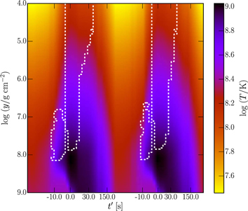
Figure 21. Kippenhahn plot during two X-ray bursts for the rp_305 net with the solar metallicity accretion model. The x-axis values are times relative to the peak of each burst, note the nonlinearity of the scale. The y-axis values are the column depth and the color coding shows the temperature of the NS envelope. The dashed contours show the extent of the convective regions.
Download figure:
Standard image High-resolution imageWe test three reaction networks, rp_53, rp_153 and rp_305, each a modified form of that in Fisker et al. (2008). Table 5 shows that increasing the number of isotopes in the reaction network increases the recurrence time and that all (for  ) have recurrence times
  less than that of GS 1826-24.
Table 5. Recurrence Times of X-Ray Bursts
| Model | Accretion Rate ( ) ) |
Composition | Recurence Time (hr) |
|---|---|---|---|
| GS 1826-24 | 4.0750 ± 0.0003 | ||
| rp_53 | 3.00 | 2% metals | 1.5 ± 0.10 |
| rp_153 | 3.00 | 2% metals | 3.3 ± 1.80 |
| rp_305 | 3.00 | 2% metals | 3.2 ± 0.07 |
| rp_305 | 3.00 | 2% 
|
3.0 ± 0.07 |
| rp_305 | 2.40 | 2% metals | 4.1 ± 0.30 |
| Heger et al. (2007) | 1.17 | 2% 
|
5.4 ± 0.10 |
Download table as: ASCIITypeset image
Figure 22 and its insert show the folded light curves for each of the three rp reaction networks plus the GS 1826-24 observations. The rise time is sensitive to the net, with the largest net matching the observed slow rise. The observed decay profile is also best matched by rp_305. Burst to burst variations of the models decrease with increasing net size and can be further reduced by increasing the temporal resolution of the models. However, increasing the size of the net reduces the variation without having to increase the temporal resolution and also highlights the impact of MESA's capability to include large nuclear networks.
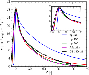
Figure 22. Folded burst profiles for the different nuclear networks as compared to GS 1826-24 for an accretion rate of  with 2% metals with a solar composition, Three rp network models are shown and one of the adaptive net models. The insert shows a zoom in of the first
  during the burst.
Download figure:
Standard image High-resolution imageTo achieve a better match to the GS 1826-24 recurrence time (see Table 5), we reduce the accretion rate to  . However, Figure 23 shows that the light curve comparisons are not as good as for the higher
  .
.

Figure 23. Folded burst light curve for the rp_305 net, with a solar metallicity accretion composition, shown for  and
and  , normalized to the peak flux measured for GS 1826-24. The insert shows the first
  of the burst.
Download figure:
Standard image High-resolution imageGS 1826-24 was also modeled by Heger et al. (2007) with accretion of hydrogen, helium and 2%  . For comparison, we run a model with this same composition with the rp_305 net. Table 5 shows that the recurrence time decreases slightly when accreting 2%
  rather than 2% metals. The model with metal accretion is in better agreement with both the light curve rise and decay.
We now explore adaptive nets (Woosley et al. 2004), where we allow MESA to determine which isotopes (and reactions) are necessary by assessing the available reaction pathways for the most abundant isotopes. The network is constructed by first finding those isotopes with an abundance above a threshold,  , and then introducing those isotopes which are connected by adding or removing protons, neutrons, or α particles. That determination is made via the additional parameters
  (i.e., neutron reactions) and
  (i.e., proton and α reactions) potentially re-adding isotopes removed with the initiating
  threshold.
Accreting solar composition material at  we follow the model to the second burst, finding a recurrence time of
  , comparable to that from the rp_305 net (Table 5). The adaptive net has a better rise time profile than the rp nets, while the rp_305 net has a better fit to the decay. This gives us confidence that the rp_305 net includes all relevant isotopes which drive the X-ray burst and thus is a useful approximation. For suitable values for the sensitivity of the adaptive net, the net limits itself to
  isotopes between bursts, which increases to
  isotopes during the burst. Variations of a factor 100 in the threshold parameters only change the isotope count by at most 50 isotopes and do not affect the final results.
6. CORE-COLLAPSE SUPERNOVAE
The capability of using large, in situ reaction networks without the need for equilibrium or co-processing techniques was described in Section 5 and applied to X-ray burst models. We extend our demonstration of this capability by first considering pre-supernova models. We then combine the advanced burning development with the implicit treatment of shocks discussed in Section 4 to core-collapse supernovae models.
6.1. Pre-supernova Evolution without QSE or NSE
Figure 24 shows the  evolution of Mi = 15 and 30
  models from the onset of carbon burning until iron-core collapse. These non-rotating, solar metallicity models used the 204 isotope reaction network described in Section 5 and MESAstar's "Dutch" mass loss prescription with η = 0.8. These models have ≈2200 cells on the MS, ≈3500 cells as the star becomes a red supergiant, and ≈2300 cells at the onset of core collapse. At core collapse the final masses are Mf = 13.0 and 15.2
  . The curves fall below the
  scaling relation because the core becomes partially electron degenerate, as indicated by tracks crossing the Fermi energy
  4 curve. Evolution toward lower density at nearly constant temperature signals ignition of a nuclear fuel.
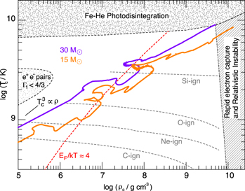
Figure 24. Evolution of  and
and  in solar metallicity, non-rotating Mi = 15 and 30
  pre-supernova models. The curves are calculated using an in situ 204 isotope reaction network. Locations of the core carbon, neon, oxygen, and silicon ignition are labeled, as is the scaling relation
  , and the
  electron degeneracy curve. Regions dominated by electron–positron pairs, photodisintegration, and rapid electron capture are shaded and labeled.
Download figure:
Standard image High-resolution imageFigure 25 shows the radial velocity and  profiles at the onset of core collapse for the Mi = 15
  model. Dashed curves show the results using a 22 isotope network and solid curves show the results using a 204 isotope network. Both models are evolved from the pre MS to the onset of core collapse with their respective reaction network. The vertical gray lines mark the mass of the iron core as defined by the
  jump, which is
  1.43
1.43  for the 204 isotope model and
  1.59
1.59  for the 22 isotope model. The infall speed has reached ≈1000 km s−1 just inside these iron core locations.
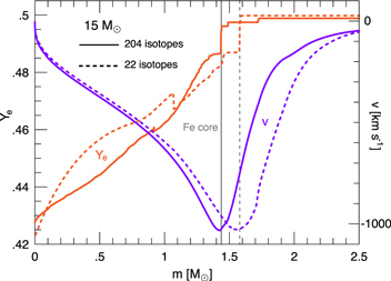
Figure 25. Radial velocity and  profiles at the onset of core collapse for the Mi = 15
  model. Dashed curves show the results using a 22 isotope network and solid curves show the results using a 204 isotope network. Both models are evolved from the pre main-sequence to the onset of core collapse with their respective reaction network. The vertical gray lines mark the mass of the iron core as defined by the
  jump.
jump.
Download figure:
Standard image High-resolution imageFigure 26 shows the thermodynamic profiles at the onset of core collapse for the Mi = 15  model. Dashed curves again show the results using a 22 isotope network and solid curves show the results using a 204 isotope network. The vertical gray lines again mark the mass of the iron core as defined by the
  jump in Figure 25. The impact of these differences remains to be explored.
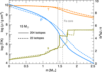
Figure 26. Thermodynamic profiles at the onset of core collapse for the Mi = 15  model. Dashed curves show the results using a 22 isotope network and solid curves show the results using a 204 isotope network. Both models are evolved from the pre main-sequence to the onset of core collapse with their respective reaction network. The vertical gray lines mark the mass of the iron core as defined by the
  jump.
jump.
Download figure:
Standard image High-resolution imageFigure 27 shows the mass fraction profiles of the ten most abundant isotopes within the iron core at the onset of core collapse for the Mi = 15  model evolved with the 204 isotope network. Each isotope shown dominates the NSE composition at some location within the iron core, although we stress that no NSE or QSE approximation was used; the same 204 isotope reaction network was used throughout the entire model from the pre-MS to the onset of core collapse.
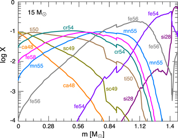
Figure 27. Mass fraction profiles of the ten most abundant isotopes within the iron core at the onset of core collapse for the Mi = 15  model evolved with the 204 isotope network. The entire iron core is in NSE and the mass fractions adapt to the changing temperature, density and
  .
.
Download figure:
Standard image High-resolution imageThe most abundant isotopes in an NSE distribution generally have an individual  that is within a small range of the local
  . A small spread usually exists due to nuclear structure effects. For example, the dominant isotopes at the center in Figure 27 are 49Sc and 48Ca. These isotopes have individual
  of 0.429 and 0.417, respectively; commensurate with the central
 0.428 shown in Figure 26. The dominant isotope changes as the NSE distribution adapts to the rapidly decreasing density profile and increasing
  profile. All the isotopes in the iron core eventually become part of the compact remnant after the explosion. However, the thermodynamic and composition profiles near the mass cut depend on the profiles interior to the mass cut.
6.2. Core-collapse Supernova Explosions
The envelope shock tests described in Section 4.9 show that the hydrodynamic solver in MESA meets the basic requirements for shock propagation in a star. The AGB star model was selected because of the well behaved conditions of its envelope—a density structure that is smooth and monotonically declining toward the stellar surface, and a uniform composition.
Here we explore the more challenging conditions associated with a strong shock born deep in the stellar interior of a massive star. We study the dynamics of such a supernova shock and the explosive nucleosynthesis that takes place in the wake of the shock during the first second. The yields from explosive nucleosynthesis depend on both the energy and the power (characteristic energy deposition timescale), while the dynamics of the shock are primarily dependent on the total energy deposited.
The starting conditions for the explosion simulations are the two 15  pre-supernova models discussed above; one for the approximate 22 isotope network and one for the 204 isotope network.
6.2.1. Explosion Dynamics
Since the focus here is on the dynamics rather than nucleosynthesis, we expedite the MESA simulation by using the 22 isotope network for both the pre-supernova and the explosion phases. Before triggering the explosion, we remove the iron core of the red-supergiant star by placing the inner boundary of the grid at a Lagrangian mass of 1.75  . We trigger the explosion by depositing 1.52 × 1051 erg at a constant rate during 1 s. The artificial viscosity is raised during the energy deposition phase (i.e.,
  = 0.01), when the shock is at small radii, and lowered in the subsequent evolution until shock breakout (i.e.,
  = 0.003). Since the binding energy of the envelope to be shocked is −3.2 × 1050 erg at the time we trigger the explosion, this choice of energy deposition yields a total energy at the end of the deposition phase of 1.2 × 1051 erg. This is generally considered a standard value for a core-collapse supernova.
Figure 28 shows that the development of the explosion is analogous to the tests using the (low-density) envelope of an AGB star in Section 4.9, but with significant quantitative differences. Here, the shock born at the edge of the iron core first travels through the dense CO-rich core. At the outer edge of the He-rich shell, the shock traverses a steep density gradient to enter the low-density H-rich envelope. Hence, the shock crosses regions with densities ranging from ∼106 g cm−3 at the edge of the iron core down to 10−10 g cm−3 at the stellar surface.
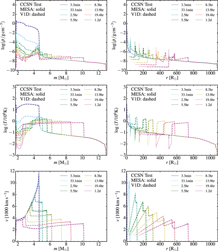
Figure 28. Multi-epoch snapshots of the hydrodynamical simulation from energy injection mimicking core-collapse supernova. The initial model is a 15  star at solar metallicity, evolved with mass loss but no rotation, and employing a nuclear network of 22 isotopes. We show the density (top row), temperature (middle row), and velocity (bottom row), vs. Lagrangian mass (left column) and radius (right column). In each panel, the solid line shows the MESA results and the dashed line the V1D results.
Download figure:
Standard image High-resolution imageThe radii of the innermost shells are initially very small since they lie at the outer edge of the iron core. Consequently, they suffer considerable cooling from expansion. Figure 28 shows a drop in temperature from a few 109 K down to ∼104 K at ∼1 day. In addition, the supernova shock splits into a reverse/forward shock structure when it encounters the density drop at the transition between the He-rich core and the H-rich envelope. The reverse shock is the new feature, absent in the envelope shock test, that causes a significant deceleration of He-core material. The conversion of kinetic energy into internal energy causes this inner material to heat up, erasing the cooling effect from expansion. The innermost layers, which travel the slowest, will be shocked last. These innermost zones can evolve to temperatures ∼104 K. It is in these innermost regions at late times that the differences between MESA and V1D are the largest. The offset occurs in a region of relatively high density (∼10−7  ) and low temperature (∼104 K). The offset in temperature between the MESA and V1D simulations at late times stems from a difference in the equation of state for metal-rich regions. MESA accounts for ionization through the OPAL equation of state table for metallicities z < 0.04. For higher metal abundances where OPAL tables are unavailable, MESA currently assumes full ionization while V1D solves for the ionization state of the gas. Note that such density/temperature regimes are normally not encountered in stellar interiors. For other quantities and/or locations/times, the agreement between MESA and V1D is excellent.
We also note that in the MESA simulation, two small spikes appear in the temperature and density profiles at <2.5  at ≈1000 s after the energy deposition phase. This feature is absent in V1D because V1D uses a much larger viscous spread when the shock is in the helium-rich core (
 ). One can reduce or eliminate such spikes by increasing the viscous spread, although this may visibly smear the shock when it crosses the H-rich envelope—the current choice seems a suitable compromise.
In contrast to the envelope shock test, this supernova explosion configuration raises the temperature by a factor of about ten. Consequently, because  , the post-shock material becomes completely radiation dominated (
 ). If we neglect the binding energy and the kinetic energy of the post-shock material, the post-shock energy is of the order of the explosion energy. We indeed find a good correspondence between the post-shock temperature computed by MESA and the temperature obtained from
  (where a is the radiation constant, E0 is a fitting parameter, typically of the order of the explosion energy, and
  is the volume within the shock radius
  ). As expected, we also find that the shock accelerates (decelerates) in regions where
  decreases (increases) outward.
6.2.2. Explosive Nucleosynthesis
Here we compare the shock nucleosynthesis results from the two independent codes, MESA and V1D. The same initial 204 isotope pre-supernova model was the starting point. Our first test case is a strong explosion triggered by injecting 1.57 × 1051 erg for 0.05 s and within 0.02  of the mass cut, which is positioned at the outer edge of the iron core at 1.5
  . The exact choice of explosion energy, deposition timescale, and mass cut is not strictly relevant.
Figures 29 and 30 compare the mass fraction profiles of MESA with a 22 isotope network, MESA with a 204 isotope network, and V1D with a 54 isotope network. The first comparison at 0.0 s shows the impact of mapping from the pre-supernova 204 isotope network to the networks used in the shock nucleosynthesis test. The next comparison at 0.05 s is at the end of the energy deposition phase. The final comparison at 42.7 s is after explosive nucleosynthesis has completed. In all cases, the silicon-rich and oxygen-rich shells are strongly influenced by the explosion; the former primarily for the production of  and the latter primarily for the production of
  and
and  . The 56Ni yields at 42.7 s are 0.092
  for V1D, 0.087
  for MESA with 22 isotopes, and 0.096
  for MESA with 204 isotopes.

Figure 29. Nucleosynthesis profiles of selected isotopes for the 1.57 × 1051 erg energy deposition test case at 0.0 s (top) and 0.05 s (bottom). The dashed lines show the MESA results with a 22 isotope network, the solid lines show the MESA results with a 204 isotope network, and the long dashed lines show the V1D results with a 54 isotope network.
Download figure:
Standard image High-resolution image
Figure 30. Same as Figure 29 but at a time after all nucleosynthesis has completed.
Download figure:
Standard image High-resolution imageOverall the agreement between MESA and V1D on this strong explosion is very good. The small differences between MESA and V1D in Figures 29 and 30 are due to the difference in mapping procedures.
MESA follows rules for mapping isotopes from one network to another network: if an isotope present in the old network is also present in the new network, then the abundance from the old network is copied to the abundance for the new network. Isotopes in the new network that are not present in the old network are initially given a mass fraction of zero. MESA then separately renormalizes classes of isotopes to have the same total mass fraction in the new network as in the old network. The classes are neutrons, hydrogen, helium, carbon, nitrogen, oxygen, and other metals. This procedure guarantees that the sum of the mass fractions in a given class will be the same in the new network as in the old network. V1D's mapping procedure for isotopes is the following. For any isotope present in the V1D network but absent in the MESA input the mass fraction is set to the solar metallicity value. When an isotope included in the MESA input is absent in the V1D network, this isotope is left out in the V1D simulation. After completing the mappings, the resulting composition is renormalized so that the sum of the mass fractions is unity.
Our second test case is a lower power explosion. We inject 1.326 × 1051 erg in 1.0 s over 0.05  of the mass cut, which is also positioned at the outer edge of the iron core at 1.5
  . The total energy after the deposition phase is 1051 erg.
In Figure 31, we show the composition profiles for the eight most abundant isotopes in the inner ≈0.4  at the end of the energy-deposition phase (i.e., at 1 s). The correspondence between MESA and V1D is again very good. The
  mass fraction approaches unity—it would reach unity if we appreciably increased the power (see Figure 29 for example). Some
  is produced in the same region, while
  is synthesized in the layers immediately above. The 56Ni yields at 1.0 s are 0.0041
  for V1D, and 0.011
  for MESA with 204 isotopes.
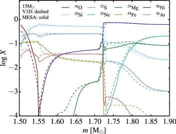
Figure 31. Composition profiles of the eight most abundant isotopes at 1 s in the inner 0.4  of the ejecta for MESA (solid) and V1D (dashed) simulations of a 1051 erg explosion in the 15
  model. The Si-rich and O-rich shells have been influenced by explosive nucleosynthesis, the former primarily for the production of
  and the latter primarily for the production of
  and
and  .
.
Download figure:
Standard image High-resolution imageThis work shows that the power of the explosion has a significant impact on the abundance profiles. In the high power explosion, the yield of  is ≈10 times larger and the
  is several orders of magnitude more abundant. The nucleosynthesis of the low power explosion is completed at end of deposition phase at 1.0 s, while nucleosynthesis in the high power case continues for ≈30 s. This sensitivity suggests potentially observable signatures between low and high power explosions. In addition, the explosive nucleosynthesis that takes place in core-collapse supernovae is sensitive to the way the explosion is triggered. With the approach we use (fixed power during the energy deposition phase), we find that increasing the explosion energy (at a given power), the power (at a given explosion energy), or both alters the amount of mass burnt. Moving the mass cut deeper into denser layers considerably enhances the amount of burnt material but this material may fall back rather than be ejected. Moving the mass cut further out into lower-density regions may completely quench the production of
  , in favor, for example, of
  . It is thus important to keep in mind that the piston or thermal explosion trigger is artificial and that the yields from explosive nucleosynthesis bear significant uncertainties.
7. IMPROVED TREATMENT OF MASS ACCRETION
Adding mass to a star requires a way to accurately and efficiently compute the thermal state of the freshly accreted material in the outermost layers. This is simplified by a hierarchy of timescales. For accretion at  , there are two important timescales at a given location, m, the thermal time
 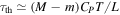 , where CP is the specific heat at constant P, and the time to accrete this same layer,
 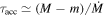 . Near the surface,
  , implying that
  , so that these layers have ample time to relax to the thermal equilibrium configuration fixed by L (Nomoto & Sugimoto 1977; Nomoto 1982; Townsley & Bildsten 2004).
In cases where L arises solely from compression of material, such as a very rapidly accreting star of high  or an old, cold accreting WD, then
  , where
  is the temperature at the degenerate/nondegenerate transition in a WD (Townsley & Bildsten 2004) or of the core in a normal star. Even in these cases, the outer layers have
  , allowing the inequality
  to hold. This also implies that the thermal state of the arriving material is unimportant, allowing us to safely use the approximation that material arrives with the same entropy as the photosphere, since material relaxes toward this on the very short
  at the photosphere.14
Even when
at the photosphere.14
Even when  varies on short timescales, using an averaged accretion rate is a good approximation for computing the evolution of the interior layers due to their long
  (Piro et al. 2005; Townsley & Gänsicke 2009).
The timescale hierarchy  implies that the outer regions evolve nearly homologously in the fractional mass coordinate
  (Sugimoto & Nomoto 1975). Hence, the thermal profile (e.g., the run of T with P or ρ) of the outer layer is nearly constant in time even as fluid elements are compressed to higher pressures and have
  increase. More formally,
  varies slowly in time near the surface, where
  . This motivates reformulating the Lagrangian based form of

that is needed in the energy equation,  (Sugimoto 1970; Sugimoto & Nomoto 1975; Paper I), to a version in the coordinate q,

Sugimoto & Nomoto (1975), and later works based on it, denote the second term on the right-hand side the "homologous" term. Physically it is the local loss of entropy in the fluid element as it is compressed to higher pressure. They label the first term on the right-hand side the "non-homologous" term. It arises from the much slower departure of the outer layers from simple homologous evolution on a timescale  .
.
MESAstar includes the ability to have an inner inert core of mass Mc. In this situation  rather than the more typical
  . For simplicity here, we will use Mc = 0. Approximate homology holds in either case for
  .
.
In Paper II, following the work of Townsley & Bildsten (2004), only the homologous term in Equation (61) was included in  in and near regions of newly accreted material. We also described the huge advantage of such an implementation, as it allows the mass added per timestep to be much larger than the smallest cell mass near the surface, while maintaining accurate thermal profiles at low pressures. However, leaving out the non-homologous term can create a discontinuity in
  at the location where the standard Lagrangian derivative, Equation (60), begins to be used. We now describe the improvement we have made to MESAstar so that it now includes both the homologous and non-homologous terms. Hence, the two forms of
  are physically equivalent and there is no longer any discontinuity.
7.1. Lagrangian and Homologous Regions
The independent coordinates used for writing the time-dependent structure of the star are m and t, and for fluid elements deep within the star at both timesteps, the conventional form of Equation (60) is adequate. One numeric subtlety of accretion is that the derivative at constant m cannot be evaluated for material that is not present in the star at the beginning of the timestep. However, the simplification available when  , manifest in Equation (61), enables
  to be evaluated in the outer regions.
When T and ρ are used as independent variables, we write

in the interior of the star, as in Paper I, and near the surface we choose to write, using Equation (61),

where

and

Here  is the T–P profile in the star, and we have used the thermodynamic derivatives
  ,
,  , and
, and  . There is also a transition region where a weighted combination of these forms is used, with weights varying linearly in m.
Placement of the transition is related to the mesh. The MESAstar mesh structure is unchanged from that discussed in Paper I and Paper II. An illustration of the mesh regions and an indication of the behavior of cell boundaries during accretion is shown in Figure 32. In the case of mass loss, analogous operations are performed; here, we focus only on mass gain.

Figure 32. Illustration of the MESAstar mesh in both m and q for a timestep in which mass is added to the star over the time interval t1 to t2. Vertical and slanted lines indicate cell boundaries. Cell size is exaggerated; there can be many cells in the newly added material. Three regions are chosen in the process of expanding the mesh for the added material, an inner Lagrangian region, an outer homologous region, and a transition region.
Download figure:
Standard image High-resolution imageA mass  is added to the star from time t1 to t2. Sizes are exaggerated for clarity; there are generally many zones in each region, possibly hundreds in the newly added material. The diagram is shown in both mass coordinate, m, and homology coordinate, q. Before each timestep, MESAstar adjusts the initial mesh resolution by splitting or merging cells based on local gradient conditions, producing an adjusted resolution mesh, which we show at t1. No simulation time elapses during that process. When constructing the mesh that will represent the star at t2, MESAstar divides the new mesh into three regions: an inner Lagrangian region, in which the m boundaries of each cell are preserved during the timestep, a transition region, and an outer, homologous region, in which the q boundaries of each cell are the same across the timestep. The result of this operation is an expanded mass domain shown at t2 in Figure 32.
Time derivatives appearing in the equations for physical evolution are then estimated using first order differences. In the Lagrangian mesh region, the finite difference form of  involves a simple same-cell difference. Similarly, in the homologous mesh region, the finite difference form of
  involves a same-cell difference. In most cases, by design, these same-cell differences are for values whose changes, e.g.,
  , are directly available from the iterative solution of the new structure, allowing us to avoid the numerical problems inherent in subtracting two almost identical numbers. In the transition region both m and q coordinates of cells have been modified, so we cannot do a same-cell difference for either
  or
or  . Instead, we interpolate values from the model at the start of the step to corresponding locations in m or q at the end of the step.
A smooth and accurate value for  in the transition region is important. To ensure this, the location of the transition region is selected to reduce the differences between the constant m and constant q forms of the time derivative and maintain accurate finite differencing. As a simple mechanism to control these, we limit, in units of cell size, the offset in the interpolation used to translate locations from the beginning to the end of the timestep (B. J. Miles et al. 2015, in preparation). Using the cell size implicitly takes advantage of the limits imposed by mesh controls on the maximum possible magnitude of cell-to-cell changes in key variables, including the variables of interest for
  time derivatives.
7.2. Testing
In order to demonstrate that the interface between the outer homologous region and the inner Lagrangian region provides a smooth profile that is independent of timestep size, we have repeated the test shown in Paper II Section 5.3. This test involves accretion of solar composition material onto a WD at  yr−1. We use the same starting model as in Paper II, which was produced by accreting hydrogen-rich material through several hydrogen shell flashes on a
  WD with an initial core temperature of about 107 K. As accretion proceeds, the total accumulated accreted mass,
  , increases up to a maximum which causes the hydrogen flash and nova runaway,
  .
.
Profiles near the transitions region are shown in Figure 33 at the time when  , which had the most severe discontinuity in Paper II. The first panel shows
  and the second panel shows
  , where HP is the pressure scale height. This is the amount of energy being released due to the
  term in the energy equation within a scale height, and has units of luminosity. We have chosen a timestep of 5000 years, which places the homology-Lagrangian transition region in a similar place to the location of the discontinuity in Paper II.
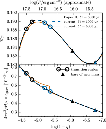
Figure 33. Profiles spanning the Lagrangian-homologous grid transition region in a  WD with a core temperature of 107 K undergoing accretion of solar composition material at a rate of
  yr−1. At the time shown
  . Shown for comparison are the results of the treatment discussed here for a 5000 years timestep and a 1000 years timestep and the treatment discussed in Paper II. For the current treatment the transition from homologous to Lagrangian is indicated by two open circles at either end of the region. The location
  in from the surface, the base of material newly accreted this step, is indicated by the triangle.
Download figure:
Standard image High-resolution imageThe orange curve in Figure 33 was computed using MESA version r4664, as used in Paper II. This displays the discontinuity due to using  from Equations (62) and (63) with only the homologous term and a transition point a factor of five deeper in pressure than
  . The black curve shows the same simulation with the same timestep for the treatment discussed here, in which
  is included and the transition region, indicated with open circles at either end, is placed as described in Section 7.1. We see that, away from the transitions,
  is unchanged from the values found in Paper II, in which only the homologous term was used in the exterior. We also show the result for a timestep of 1000 years is indistinguishable on this plot; the
  profile differs by a fraction of a percent at the edges of the transition region, and less elsewhere. In the current treatment the profiles are independent of timestep size.
8. WEAK REACTIONS
The rates module provides weak reaction rates for hundreds of isotopes. By default, when atoms are fully ionized, these rates are based (in order of precedence) on the tabulations of Langanke & Martínez-Pinedo (2000), Oda et al. (1994), and Fuller et al. (1985). These tables span a wide range of density and temperature,  and
and  , but are relatively coarse, with 11 points in the
  dimension (
 ) and 12 points in the T dimension (
 ).
).
These grids include the thermodynamic conditions where the electrons are degenerate and relativistic, which are realized for example in massive WDs and cores of intermediate mass stars. Under these conditions, the rates of electron-capture and beta-decay reactions are sufficiently sensitive to density and temperature that they can change by tens of orders of magnitude between adjacent points in these tables. Linear or cubic interpolation cannot accurately reproduce the value of the rate between the tabulated points.
The difficulty of interpolating in coarse rate tabulations was discussed by Fuller et al. (1985), who proposed a physically motivated interpolation scheme, hereafter referred to as Fuller, Fowler, and Newman (FFN) interpolation. Their procedure assumes the rate has the form given by a single transition between the parent and daughter nuclear ground states. However, the true rate may be dominated by allowed transitions to or from excited states in the parent or daughter nucleus. This is almost always the case when the ground state to ground state transition is highly forbidden. The specific transition that dominates the rate may change over the range of thermodynamic conditions covered by the table. The FFN interpolation method does not account for these complications.
Figure 34 compares the results of the interpolation methods described in the preceding paragraphs with the on-the-fly approach that we have implemented in MESA and will be described here. It shows the electron-capture rate on  and beta-decay rate of
  at fixed temperature. Linear interpolation of these coarse tables fails to reproduce the rapid variation in the rate. The FFN interpolation method produces curves with characteristic shapes more similar to the true rate, but because the Q-value is that of the ground state to ground state transition and not that of the transition that dominates the rate, the density dependence is not correct in detail.
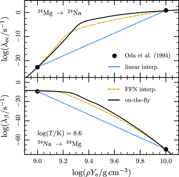
Figure 34. Top panel (bottom panel) shows the rate of electron capture on  (beta decay of
  ) as a function of density at a fixed temperature of
  . The Oda et al. (1994) tabulated points are shown as black dots. The dotted line shows the result of using linear interpolation between the tabulated points. The dashed line shows the result of using the physically motivated interpolation method suggested by Fuller et al. (1985). The solid line shows the rate calculated using the on-the-fly rate calculation capability of MESA documented in this section. Slight differences between points and the line are due to differences in the input nuclear data.
Download figure:
Standard image High-resolution imageIn recent years, a number of authors have discussed the importance of well-sampled weak rates in capturing the influence of these processes on stellar evolution. This can be achieved by generating denser tables for the specific reactions of interest or by using analytic approximations to the rates (e.g., Toki et al. 2013; Martínez-Pinedo et al. 2014). We now present a capability by which MESA can calculate weak reaction rates on-the-fly from input nuclear data. This removes the potential for interpolation artifacts. It also enables easy experimentation in cases where the input nuclear data may not be well-measured. We begin with an overview of how we calculate these weak rates and illustrate their utility and a few applications.
8.1. Calculation of Weak Rates
Consider two nuclei  and
and  that have two states connected by an electron-capture transition

and beta-decay transition

The energy difference between the ground states can be written as

where MA and MB are the nuclear rest masses of the ground states. The total energy difference between any two states can be written as

where Ei and Ef are the energies of the initial and final states measured relative to the ground state. For the transitions that we consider here,  and
and  for electron capture and
  and
and  for beta decay.
In this section, we use J to represent the nuclear spin. We work in the allowed approximation, which neglects all total lepton angular momentum (L = 0). This restricts us to Fermi transitions, where the total lepton spin is S = 0, and therefore the initial and final nuclear spins are equal ( ), and Gamow–Teller transitions, where S = 1, and therefore
  (excluding
  ). In both cases, there is no parity change:
  (e.g., Commins 1973).
The total rate of the process (electron capture or beta decay) is the sum of the individual transition rates from the ith parent state to the jth daughter state,  , weighted by the occupation probability of the ith parent state, pi.

where  is the comparative half-life and can be either measured experimentally or calculated from theoretical weak-interaction nuclear matrix elements. The i-sum is over all parent states and the j-sum is over all daughter states. The occupation probability is

where we define  . The quantity Φ is a phase space factor which depends on the electron chemical potential
  (including the electron rest mass), on the temperature T, and the energy difference Qij. The value of Φ for electron capture is

where α is the fine structure constant. For beta decay it is

Similarly, the total rate of energy loss via neutrinos is

The value of Ψ for electron capture is

and for beta decay it is

In order to implement these equations in MESA, we rewrite the integrals in terms of Fermi–Dirac integrals, following Appendix A of Schwab et al. (2015). MESA implements fast quadrature routines to evaluate integrals of this form. Each time a weak rate is needed, it is calculated on-the-fly. We discuss the computational cost of this procedure in Section 8.3.
Assuming thermal equilibrium, the energy released by weak reactions depends only on total reaction rate, total neutrino loss rate, energy difference between the nuclei, and the electron chemical potential. Therefore, the total specific heating rate from a reaction is


where nA and nB are the number densities of the species undergoing electron capture and beta decay, respectively, and ρ is the total mass density.
Therefore, given a list of nuclear levels and the  -values for the transitions between them, MESA can calculate the rates of electron capture and beta decay and the corresponding energy generation rates. Typically only a few low-lying states and the transitions between them are needed. As an example, Figure 35 shows the rates for the
  –
– Urca pair.
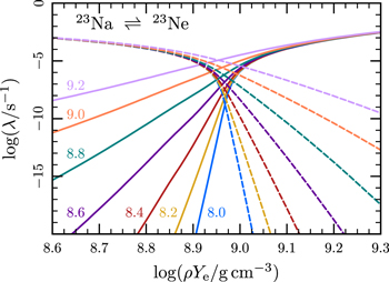
Figure 35. Electron capture (solid lines) and beta decay (dashed lines) rates of the  –
– Urca pair as calculated by MESA, using the on-the-fly methods described in this section. The value of
  is shown next to each electron capture line; the beta decay line of matching color is at the same temperature. The rates vary rapidly, with both temperature and density, near the threshold density, which is roughly in the center of the plot.
Download figure:
Standard image High-resolution image8.1.1. Coulomb Corrections
In a dense plasma, the electrostatic interactions of the ions and electrons introduce corrections to the weak rates relative to those which assume a Fermi gas of electrons and an ideal gas of ions. Our treatment of these effects, which is presented in Appendix B of Schwab et al. (2015), is similar to Appendix A of Juodagalvis et al. (2010).
Since electron capture and beta decay change the ion charge, the Coulomb interaction energy changes the energy difference between the parent and daughter nuclear states. To calculate this shift, we use the excess ion chemical potential  from Potekhin et al. (2009). We incorporate this effect by shifting the value of Qij, as defined in Equation (69), by an amount
  . This shift,
  , enters the calculation of the phase space factors and the energy generation rates.
The electron density relevant to the reaction rate is not the average electron density, but rather the electron density at the position of the nucleus. This correction is accounted for as a shift in the value of the electron chemical potential that enters the phase space factor,  . Values of Vs have been calculated by Itoh et al. (2002). This correction does not enter the energy generation rates because it has not changed the energy cost to add or remove an electron.
8.2. Applications
When  , only the few electrons in the tail of the Fermi–Dirac distribution have sufficient energy to overcome the energy gap and capture on A to form B. Thus, the rate of electron capture is small compared to the rate of beta decay, and so isotope B is favored in the equilibrium. When
  , there are only a few unoccupied states available to accept the energetic electron from the beta decay. This final state blocking means the rate of beta decay is small compared to the rate of electron capture, and so isotope A will be favored in the equilibrium.
The shift in this equilibrium can have profound consequences when it occurs in stellar interiors. It modifies the composition, reduces the electron fraction, and alters the thermal state of the plasma. We now discuss two applications of our on-the-fly treatment of the weak rates: the Urca process and accretion-induced collapse.
8.2.1. Urca Process
When the ground state to ground state transition is allowed (odd nuclei), the rates of electron capture and beta decay are both significant when  . Since each reaction produces a neutrino which free-streams out of the star, this can lead to significant cooling. With a total number density of an Urca species
  , assuming the abundances are given by the detailed balance condition
  , the volumetric neutrino cooling rate will be
  , where

In the limit  , the maximum value of the Urca cooling rate at a given temperature has a simple form (e.g., Tsuruta & Cameron 1970)

Well-sampled rates such as those shown in Figure 35 are necessary to reproduce the correct Urca cooling rates. We illustrate this in Figure 36, which shows Cmax for the  –
– Urca process for temperatures 108–109 K. The circles show the results using the on-the-fly treatment described in this paper; the squares show the results using the coarse tables of Oda et al. (1994). The dashed line shows the cooling rate expected from Equation (80) which is in excellent agreement with the results of the on-the-fly method. The Urca cooling rates calculated from interpolating in coarse tables severely underestimate the true cooling rate when
  .
.
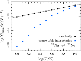
Figure 36. Effect of the interpolation method on the Urca process cooling rates. The circles show the maximum value of C (Equation (79)) calculated using the on-the-fly methods discussed in this section; the squares show the results using the coarse tables of Oda et al. (1994). Interpolation in these coarse tables severely underestimates the Urca cooling rates at low temperatures. The dashed line shows the expected value of the cooling rate given by Equation (80).
Download figure:
Standard image High-resolution imageThus, when the Urca process is important, well-resolved weak rates are necessary to correctly capture the temperature evolution of the core (Jones et al. 2013; Toki et al. 2013). Jones et al. (2013) used MESA r3709 along with a denser table described in Toki et al. (2013) to do their work. The Toki et al. (2013) table is not publicly available, so to reproduce the results of Jones et al. (2014) we save a model of an 8.8  star at
  from our run with MESA (version r3709) using the Jones et al. (2014) inlists. We then load this model into a newer MESA version (r7503) that has access to the on-the-fly weak rates and evolve this model using a network with only the Urca process reactions. During this phase other nuclear reactions are not important to the central evolution.
Figure 37 shows the central temperature and density of the core. The solid lines show the evolution using the on-the-fly rates, the dashed lines show the results when interpolating in coarse tables. The drops in temperature at  and
and  correspond to cooling from the
  –
– and
and  –
– Urca pairs, respectively. The corresponding shifts in composition can be clearly seen in the lower panel. These results demonstrate the importance of densely sampled weak rates to the evolution of the core.

Figure 37. Top panel shows the evolution of  and
and  in an 8.8
  star. The bottom panel shows the central
  and
and  mass fractions. The solid lines show the evolution using the on-the-fly rates, the dashed lines show the results when interpolating in coarse tables. The locations of the changes in mass fraction match the locations of cooling in the top panel. This demonstrates the importance of densely sampled weak rates to the evolution of the core.
Download figure:
Standard image High-resolution image8.2.2. Accretion-induced Collapse
When the ground state to ground state transition is forbidden (even nuclei), the first transition to become significant is typically an allowed transition into an excited state. In these cases, the beta decays from the daughter ground state are blocked and decays from daughter excited states are strongly suppressed by the Boltzmann factor. Therefore significant cooling via the Urca process does not occur. Instead, since the captures are preferentially to an excited state, significant heating occurs via gamma-ray emission as level populations relax to a thermal distribution.
Two important capture chains occur in oxygen-neon-magnesium (ONeMg) cores:  and
and  . For these sequences of captures, the excess electron energy is thermalized. These are the key reactions in electron-capture supernovae and the accretion-induced collapse (AIC) of ONeMg WDs (e.g., Miyaji et al. 1980). As the degenerate core approaches the Chandrasekhar mass, the electron captures remove the pressure support and heat the plasma. Figure 38 shows the evolution of a cold ONeMg WD (
 ,
,  ,
,  ) accreting at
  . The solid lines show the evolution using the on-the-fly rates described in this section; the dashed lines show the results when interpolating in coarse tables. When using the coarse tables, the electron captures on
  do not occur until approximately a factor of two larger density. At this greater density, the energy deposition from each capture is higher and this leads to a large temperature change due to the A = 24 captures alone. In contrast, the on-the-fly rates show the behavior demonstrated in previous studies of this evolution that did not use sparse tables (e.g., Miyaji & Nomoto 1987): the A = 24 captures heat the plasma and accelerate the contraction; the A = 20 captures, due to the higher
  abundance and a higher energy release per capture, cause a thermal runaway and the formation of an oxygen deflagration (Schwab et al. 2015).

Figure 38. Evolution of a cold ONeMg WD toward AIC. The top panel shows the evolution of  and
and  . The bottom shows the central
  and
and  mass fractions. The solid lines show the evolution using the on-the-fly rates; the dashed lines show the results when interpolating in coarse tables.
Download figure:
Standard image High-resolution image8.3. Guidelines
MESA provides the nuclear data used in the calculation of the reactions specifically discussed in this section (Tilley et al. 1998; Firestone 2007a, 2007b, 2009; Shamsuzzoha Basunia 2011; Martínez-Pinedo et al. 2014). To consider additional reactions, a list of nuclear levels and  -values must be specified.
The expressions in Section 8.1 assume degenerate, relativistic electrons. As  increases, additional transitions to higher energy states of the daughter nuclei and must be included. At higher temperatures, excited states of the parent nucleus will begin to be thermally populated and captures or decays from those states and must be included. At temperatures and densities where the composition approaches NSE, these methods are particularly inappropriate, as it is necessary to consider large pools of isotopes (Juodagalvis et al. 2010).
9. CHEMICAL DIFFUSION
MESA's early implementation of microscopic element diffusion incorporated the approach used by Thoul et al. (1994) in their seminal work on understanding the sedimentation of helium in the solar interior. The fundamental starting point for this treatment of diffusion is the Boltzmann equation with the assumption of binary collisions where the particle's mean free path is much larger than the average particle spacing. This formalism, encoded in the Burgers equations (Burgers 1969), assumes that ions interact with an effective potential that governs isolated interactions between only two particles at a time. For more strongly coupled plasmas, as  exceeds unity (where
  is the mean inter-ion spacing, and
  is the total ion number density), it is no longer clear that this assumption remains valid. Later updates to MESA incorporated the work of Hu et al. (2011) on radiative levitation and incorporated the resistance coefficients calculated by Paquette et al. (1986) for approaches to the denser plasma regime as
  .
.
Here we describe MESA's current implementation of chemical diffusion and then discuss the path forward for diffusion implementations in the  regime, needed for accurate studies of diffusion in the interiors of WDs or surfaces of NSs. Recent theoretical work in this strongly coupled regime (Baalrud & Daligault 2013, 2014; Beznogov & Yakovlev 2014) provides support for a future update of MESA.
9.1. Current Methods in MESAstar
We now describe the formalism and assumptions underlying the approach to diffusion currently present in MESA. This is followed by a discussion of the framework for numerical implementation of this formalism provided by Thoul et al. (1994) and key modifications present in the current version of the MESA diffusion routine.
9.1.1. Burgers Equations and the Low Density Limit
The Burgers equations for diffusion in an ionized plasma are derived using the Boltzmann equation for the distribution function  for particles of type s

where xi are the components of the position vector,  are the components of the velocity vector, fsi are components of the forces on particles of type s, and ms is the mass for those particles. Throughout this section, the indices s and t refer to particle species, while i and j are used to index other quantities such as spatial components of vectors.
Burgers adopts the 13-moment approximation due to Grad (1949) as a closure scheme for taking moments of the Boltzmann equation. Burgers also assumes an approximately Maxwellian distribution function

where  ,
,  represents the components of the deviation of the velocity from the mean flow velocity
  of the species, and

is the small deviation ( ) from the Maxwellian distribution. The coefficients Bsij and Csi are defined such that the distribution function has a total of 13 free parameters corresponding to the 13 moments of the closure scheme (see Burgers 1969).
Burgers derives the collision integrals ( ) and cross-sections (
 ) that result from taking moments of the right-hand side of the Boltzmann equation


where  ,
,  , v represents the relative velocity of colliding particles, and the angle of deviation
  is a function of both v and the impact parameter b that depends on the physics of the two-particle interaction between colliding particles in the gas. Burgers then defines the dimensionless coefficients zst,
  ,
,  , and
, and  , along with resistance coefficients ( Kst) in terms of the collision integrals:

In the "single-fluid picture" the diffusion velocities are defined with reference to the mean velocity of the gas as a whole ( ), rather than with respect to the mean species velocity (
 ):
):

Burgers defines residual heat flow vectors

As shown in Section 18 of Burgers (1969) if we assume  and the absence of magnetic fields, the basic equations of diffusion are


where  is the quasi-static electric field and
  is the average charge density of species s. These equations are still general, with the form of the resistance coefficients not yet fully specified. The physics of the particular types of interactions within ideal gases is fully contained in the coefficients Kst, zst,
  ,
,  , and
, and  .
.
For ionized gases, the resistance coefficients require evaluation of collision integrals that diverge for a pure Coulomb potential. However, since the two-particle interaction potential is only truly applicable on short length scales, an integration cutoff or screened potential is commonly adopted. Burgers chooses to calculate resistance coefficients using a pure Coulomb potential truncated at the Debye radius

which is assumed to be much larger than the inter-ion spacing. Indeed, for a plasma of one species,  . Applying this form of interaction to the collision integrals, the l = 1 integrals defined in Equation (84) can be evaluated (Baalrud & Daligault 2014)

where 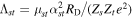 . In order to perform the integral in Equation (85), Burgers notes that the dependence of
  on v inside the logarithmic term is weak, so that we can replace v2 there with its average value
  . Assuming a very dilute plasma, so that
  , Burgers then writes

and the final result for the resistance coefficients follows as


With these coefficients now fully specified, Burgers diffusion equations along with constraints such as charge neutrality and current neutrality form a closed set of equations, which can be solved for  ,
,  ,
,  , and
, and  from the input of a stellar profile.
9.1.2. MESA's Implementation of Thoul et al.'s Approach
The diffusion routine originally implemented in MESA was based on the work of Thoul et al. (1994). They start with the Burgers equations, written in a compact notation following Noerdlinger (1977, 1978) that is equivalent to Equations (89) and (90) in one dimension. However, the approach of Thoul et al. (1994) differs from Burgers' original treatment in one important respect: the resistance coefficients are based on a modified result for the collision integrals. They follow Equation (95) for the various zst coefficients, which uses a pure Coulomb potential with a cutoff at the Debye length, but the Kst coefficients were derived from an alternative fitting of the Coulomb logarithms introduced by Iben & MacDonald (1985). For these coefficients, they define 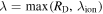 , and use

This expression is a fit to the numerical results of Fontaine & Michaud (1979), motivated by WD conditions where Burgers' approximations for dealing with Equation (92) are not valid ( ). Since this fit focuses on the strong coupling regime, and differs from Equation (94), these results can be incorrect in the limit of a dilute plasma as we discuss later. Nevertheless, Thoul et al. (1994) elected to use Equation (96) under all conditions, since it provides an approximately correct solution in a convenient closed form.
Using Equations (89) and (90) along with the constraints of current neutrality ( ) and local mass conservation (
 ), Thoul et al. (1994) express an entire closed system of equations in a dimensionless matrix form suitable for numerical evaluation:

where S is the total number of species in the gas (including electrons) and  is the concentration of the jth species. Consult Thoul et al. (1994) for definitions of K0,
  ,
,  ,
,  , and
, and  . The definition of Wj is
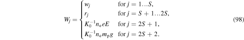
This is the vector containing the unknown quantities solved for after specifying K0,  ,
,  ,
,  , and
, and  . The routine provided by Thoul et al. (1994) inverts Equation (97) for one term in the left-hand side at a time so as to find the "generalized diffusion coefficients," which can be used to construct diffusion velocities or contributions from pressure, temperature, or concentrations individually.
9.1.3. Modified Coefficients and Radiative Levitation as Implemented by Hu et al.
Hu et al. (2011) extend the methods of Thoul et al. (1994) by introducing some key modifications. First, they include an extra force term due to radiative levitation, so that Equation (89) becomes
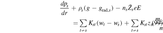
where  refers to the radiative acceleration on species s.
  is the average charge of species s, allowing an account of partial ionization so that
  . They do not modify Equation (90).15
In contrast to Thoul's original routine, Hu et al. (2011) use the resistance coefficients from Paquette et al. (1986), which were generated based on substantial improvements to Fontaine & Michaud (1979). In evaluating the collision integrals, Paquette et al. (1986) use a screened Coulomb potential of the form

where, once again,  . As we note below, this choice of λ makes a substantial difference in strongly coupled plasmas, where the Debye radius no longer corresponds to a distance at which other nearby charged particles can significantly screen the Coulomb field. After setting up the algebra for a matrix solution very similar to that of Thoul et al. (1994), Hu et al. (2011) solve for the vector Wj (as defined in Equation (98)) appearing in the equation
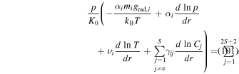
Many of the quantities appearing in this equation are defined differently than in Thoul et al. (1994); see Hu et al. (2011) for details. We can also solve this equation directly for the vector Wj to obtain

the strength of the electric field relative to gravity.
9.2. Analytic Expression for the Electric Field
In some simple cases, Burgers equations can be solved to yield an analytic expression for the electric field, providing a useful test for MESA. Starting directly with his diffusion equations, Burgers (1969) arrives at the following expressions for a pure plasma of electrons along with one species of ions (charge Ze):


where  . For a plasma with only one ion species in diffusion equilibrium, the constraints of current neutrality and local mass conservation give
  . In the case of a pure hydrogen plasma,
  , and in hydrostatic equilibrium
 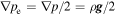 . Hence, we can solve the above set of equations to find

The coefficient for the temperature gradient term depends directly on the nature of the resistance coefficients in the Burgers formalism, so different models of Coulomb collisions in ionized plasma will lead to different results for the electric field.
As a slight generalization of Equation (105) in one dimension, we write

If we calculate the coefficient  using the Burgers' formalism with Equations (95) and (96), we find

A comparable analytic expression for the electric field is provided by Roussel-Dupré (1981), who applies a Boltzmann–Fokker–Planck approach to finding diffusion coefficients for trace elements in hydrogen plasma. His treatment of diffusion is more precise than the Burgers' formalism, but has the limitation of only being applicable in the case of nearly pure hydrogen with a diffusing trace element. His result for the electric field matches the form of Equation (106) with the coefficient  . This provides another useful point of comparison in the specific case of nearly pure hydrogen plasmas. Below we use this analytic expression as a test of the updated resistance coefficients employed by Hu et al. (2011).
9.3. Results and Comparisons
We have constructed several simple MESA test cases in order to illustrate the effects of radiative levitation and different resistance coefficients. Where possible, we compare MESA output to corresponding analytic expressions.
9.3.1. Electric Fields
By default, MESA uses the resistance coefficients provided by Paquette et al. (1986), but it can also use the resistance coefficients defined by Iben & MacDonald (1985), given here in Equation (96). In the case of a pure hydrogen star, the coefficients given in Equation (96) lead directly to Equation (107), so these coefficients are especially useful in performing simple comparisons of MESA output to a corresponding analytic expression. Due to the complicated numerical methods used to obtain the resistance coefficients of Paquette et al. (1986), it is not possible to write down a directly corresponding closed form analytic expression for the electric field, but results based on these more precise calculations compare favorably to those of Roussel-Dupré (1981) in the case of a pure hydrogen plasma. Starting with the MESA test suite, we constructed a solar mass pure hydrogen star, and we ran just long enough to turn on the diffusion routine and gather output for electric and gravitational fields. For such a star, we can compare MESA results for the electric field directly to the analytic expression given in Equation (106), with  in the solution of Burgers (1969) and
  for Roussel-Dupré (1981).
Figure 39 plots the result of Equation (106) for both values of  , along with the results from the diffusion routine (Equation (102)) for each type of resistance coefficients available in MESA. As expected, the curve calculated from the MESA diffusion routine output using the resistance coefficients of Iben & MacDonald (1985) closely matches the analytic expression with
  as calculated by Burgers (1969) using his similar coefficients. When using the more detailed numerical calculations for the resistance coefficients provided by Paquette et al. (1986), the diffusion routine output closely resembles the more precise analytic calculation given by Roussel-Dupré (1981).
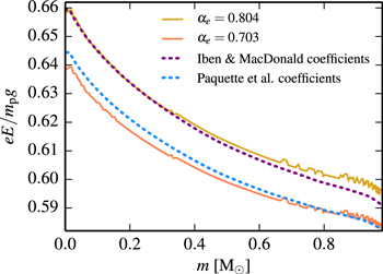
Figure 39. Comparison of electric field strengths relative to gravity in a pure hydrogen star ( ,
,  ,
,  ) with nuclear burning artificially suppressed in the MESA routine to avoid any helium contamination. Solid lines represent the analytic expression given by Equation (106) for two different values of the coefficient
  . Dashed lines represent output from the MESA diffusion routine as described in Equation (102), with the only difference being the resistance coefficients used to solve the Burgers equations.
Download figure:
Standard image High-resolution imageThe Sun provides another interesting test case for comparing the effects of using different resistance coefficients. An example solar model from the MESA test suite was run with different choices of the resistance coefficients. Figure 40 shows a slight difference between the electric field strengths relative to gravity given by the Paquette et al. (1986) coefficients and those by Iben & MacDonald (1985).
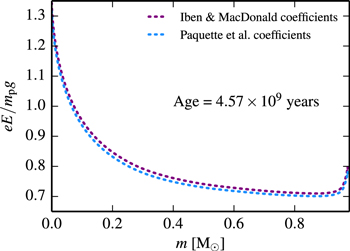
Figure 40. Comparison of electric field strengths relative to gravity using different resistance coefficients in a solar model.
Download figure:
Standard image High-resolution image9.3.2. Gravitational Fields
The MESA diffusion routine treats both the electric field and local gravitational acceleration as unknown quantities. MESA records the quantity  (Equation (98)), used to calculate the gravitational acceleration from the diffusion routine:

This expression for  is independent of the simpler expression for local gravitational acceleration
  . Figure 41 compares gGauss and gdiff for a typical profile found using the example solar model from the MESA test suite. In Figure 41, a profile from a star of larger mass (
 ) shows disagreement between the gravity outputs in the convective core. The Burgers formalism assumes heat transfer that is correlated with temperature gradients through the residual heat flow vectors defined in Equation (88). This assumption breaks down when most of energy is transported by convection; however, the effects of diffusion in this region are completely overwhelmed by convective mixing and are therefore inconsequential.

Figure 41. Comparison of gravitational fields obtained from  and
and  in two MESA test suite cases. The two lines representing the Sun (
 ) show good agreement, while the two lines representing a
  star disagree in regions with large convective flux where diffusion is inconsequential.
Download figure:
Standard image High-resolution image9.3.3. Radiative Levitation
MESA's implementation of radiative levitation is based on Hu et al. (2011). Figure 42 shows an abundance profile of a subdwarf B star model produced by MESA, where radiative levitation is responsible for the presence of  ,
,  , and other metals near the surface (as also seen in Figure 3 of Hu et al. 2011).
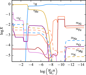
Figure 42. Abundance profile of a subdwarf B star model ( ,
, 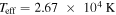 ,
,  ,
,  ) showing the effects of radiative levitation with a layer of
  at the surface.
Download figure:
Standard image High-resolution image9.3.4. WD Sedimentation
In a cooling WD, diffusion governs sedimentation over long timescales. The assumptions behind the formalism of the Burgers equations do not hold under WD conditions.
- 1.The Burgers equations assume all particle species satisfy an ideal gas equation of state. In the context of a degenerate WD both electrons and ions violate this assumption.
- 2.The very dense, strongly coupled (
 ) conditions of a WD call into question the validity of the two-particle scattering picture used to calculate the ion resistance coefficients.

Nevertheless, for lack of a better option, previous studies have relied on the Burgers equations with the coefficients of Paquette et al. (1986). For example, see Córsico et al. (2002).
Figure 43 shows an abundance profile produced by MESA for a CO WD after 4 Gyr of evolution, where diffusion governs sedimentation in the outer layers. The vertical lines in Figure 43 mark the outer boundaries of regions where the two concerns listed above become significant. Nearly all of the WD resides inside at least one of these regimes, and much of the interesting diffusion sedimentation occurs inside regions that are both significantly coupled and highly degenerate. Thus, improvements to the treatment of diffusion are clearly necessary before we are able to describe diffusion in WDs adequately. This MESA run turns off diffusion for  , where we expect strong coupling to substantially modify the underlying equations.
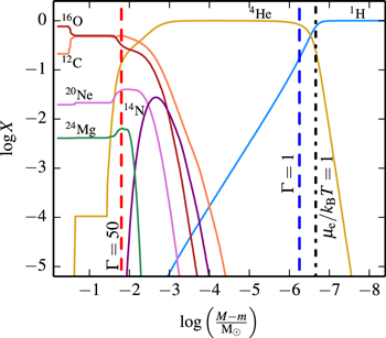
Figure 43. Abundance profile of a CO WD (M = 0.611  ,
,  = 5.16 ×
  ,
, 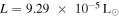 ) after 4 Gyr of WD evolution. The region left of the blue, dashed line is the interior of the WD, where
  . Left of the red, dashed line
  , and diffusion has been turned off for this region. The electrons are an ideal gas to the right of the black dotted–dashed line.
Download figure:
Standard image High-resolution image9.4. Expanding the Domain of Validity and Next Steps
The validity of the Boltzmann approach becomes questionable as  and the ions become a liquid. Bildsten & Hall (2001) estimated the diffusion coefficient in this liquid regime by using the Stokes–Einstein relation. However, for a broad-based code such as MESA, we need to implement diffusion into the
  regime in a manner that allows for a smooth transition between coupling regimes.
Paquette et al. (1986) successfully described diffusion in a regime of intermediate coupling through the use of screened potentials, which are a way to account for the collective nature of interactions in a dense plasma. Though there is no rigorous reason to expect that a formalism based on the two-particle scattering picture should work well as  , their comparison to simulations verified that this description of diffusion is very accurate for
  .
.
Can these approximations be extrapolated to the strongly coupled regime of  ? Baalrud & Daligault (2013) provide a method for numerically calculating resistance coefficients using a hypernetted chain (HNC) approximation from effective potentials. Figure 44 compares their HNC results (diamonds) to their Molecular Dynamics (MD) simulations of a one-component plasma (OCP, circles) for the self-diffusion coefficient
  , defined by

where  is the plasma frequency and
  (the factor of 2 in this definition ensures that if we redefine species s in terms of two subspecies s1 and s2, then
  ). The general expression for the interdiffusion coefficient is

where the  term in the denominator accounts for a second order correction that can be defined using

For reference, we also include a direct fit of Daligault & Murillo (2005) to the MD data of Ranganathan et al. (2003), given by

The agreement between the HNC and MD simulations shows that the HNC does a better job of accounting for correlation physics in strongly coupled plasmas than a simple screened Coulomb potential and allows for a surprising (and still physically unexplained) extension of the Burgers formalism into the strongly coupled regime. This recent work allows us to go into the large Γ limit with the Burgers formalism, but the question remains as to how we obtain diffusion coefficients in a reliable manner.
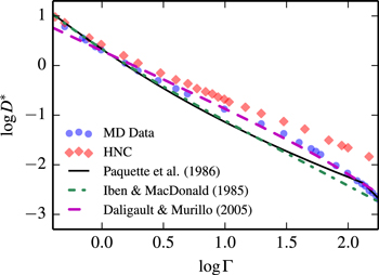
Figure 44. Compilation of the self-diffusion coefficients obtained from different methods. "MD Data" and "HNC" points are taken from Baalrud & Daligault (2013). The solid black line is the result of the MESA calculation using the coefficients of Paquette et al. (1986). The dashed green line is the result of the calculation using the resistance coefficients from the original routine of Thoul et al. (1994) based on the fit to the Coulomb logarithm found in Iben & MacDonald (1985), given here in Equation (96). The dashed purple line represents the fit to MD data given here in Equation (112).
Download figure:
Standard image High-resolution imageThe self-diffusion coefficients from the two options in MESA are shown in Figure 44 and correlate with the MD data better than expected for the high Γ regime. In particular, the agreement is much better than that shown in Figure 2 of Baalrud & Daligault (2013) for either "cutoff" or "screened" Coulomb methods. The reason for this agreement is that both MESA implementations use the inter-ion spacing rather than the Debye length once  , which yields favorable scalings in the high Γ limit. Iben & MacDonald (1985) constructed their fitting formula based on a few numerical results for
  1. Paquette et al. (1986) also showed that their formalism can be extended to
  as long as the inter-ion spacing is used rather than the Debye radius for the screening length.
Though MESA does not yet provide the capability of implementing resistance coefficients based on the HNC method, we hope to accomplish this in the near future by means of a table similar to that provided for the coefficients of Paquette et al. (1986). For a more thorough discussion of these methods and the likely path of application to mixtures, consult Beznogov & Yakovlev (2014). We will also need to correctly account for the electron degeneracy and the non-ideal equation of state for the ions, both of which modify the electrostatic field needed to correctly determine the forces that drive diffusion.
10. SOFTWARE INFRASTRUCTURE
Here we describe a number of changes to MESA that have occurred since Paper II and are of potential interest to users of MESA or developers of similar software.
MESA can be compiled with either the GNU or Intel Fortran compilers, runs on multiple operating systems (Windows, OS X, and Linux), and can use different numbers of OpenMP threads. It is necessary to regularly test that the code is performing correctly across the different combinations of compiler, OS, thread count. To this end, developers and engaged users run the MESA test suite on a wide range of systems before each release.
Previously, test cases in the MESA test suite accepted different results so long as they were within a certain tolerance, an appropriate choice for testing scientific results where the physical uncertainties are much greater than the numerical ones. However, we found that this made detecting and tracking bugs across platforms difficult. For the purposes of code testing, it is much better to insist that any inconsistency is a problem, no matter how small.
Motivated by this challenge, MESA now provides bit-for-bit consistency for all results across all the supported platforms. It is essential to emphasize that the goal of this achievement is to enable better testing. It allows users to exactly reproduce the results of others, independent of platform differences, which is especially useful to developers attempting to reproduce bugs. The achievement of bit-for-bit consistency is not a claim that the results of MESA calculations are physically accurate or numerically converged to any specific degree.
This bit-for-bit consistency was achieved via the following choices.
- 1.Using parallel algorithms that give identical results independent of number of threads or order of thread execution. MESA's linear algebra solver is based on BCYCLIC (Hirshman et al. 2010). It sub-divides the work between threads based on the the size of the matrix rather than on the number of threads available. It is also necessary to avoid OpenMP reduction clauses, which provide no guarantees on ordering of operations.
- 2.Specifying compiler flags that forbid the compiler from making any optimization that can affect floating point precision (e.g., forbid re-association and fast math operations). Most optimizations are still allowed.
- 3.Using an I/O library that does precise conversion from binary to ASCII for double precision numbers.
- 4.Using a math library that gives consistent results for operations such as log, exp, sin, cos, pow. MESA uses CRLIBM16 in round toward zero mode. The choice to use a math library that gives exact results is not because 16 digit accuracy from the math routines in necessary. Rather, we want consistent results across supported platforms and this is the best way to achieve this consistency.
- 5.Replacing integer power expressions (i.e., x**3) by repeated multiplications (i.e., x*x*x). Different compilers implement integer powers differently, giving different results.
Having achieved bit-for-bit identical results, we can test files for exact equality. This applies both to the module-by-module tests that run at installation time and the case by case tests in the star and binary test suites. These test cases compare the final model from the test run to a saved result from a previous MESA version. If they are not exactly the same, the test fails. The test is also restarted from an intermediate state to confirm that runs which are stopped and restarted yield exactly the same results as those that are not.
While MESAstar is parallelized via OpenMP, the install process has historically been serial. MESA contains approximately 1000 Fortran files and so the ability to compile more than one file simultaneously has the potential to provide significant reductions in the time needed to install MESA. Recently the compilation step has been parallelized, enabled by the automated dependency generation tool makedepf90,17 allowing multiple instances of the Fortran compiler to be invoked simultaneously. This is of particular utility for developers who may recompile MESA frequently.
Since Paper II the main MESA website18 has undergone significant revision, making it easier for new users to get started with MESA. This restructuring has also made it easier for the developers to keep material up-to-date as MESA evolves. One of the most important improvements is that the files that document the default value of each MESA option use the Markdown19 markup language. This allows documentation web pages to be generated automatically for each MESA release.
Improvements have also been made to the distribution of MESA. Previously, MESA was available only by checking out the source code using the Subversion20 version control system. Now, every release version of MESA (including past releases) is available for download as a ZIP archive. This is simpler and saves bandwidth and disk space. It has quickly become the preferred way to install MESA with the ZIP file of the current release being downloaded tens of times per week.
11. SUMMARY AND CONCLUSIONS
We have explained and, where possible, verified or validated, major new capabilities and improvements implemented in MESA since the publication of Paper I and Paper II. These advancements include interacting binary systems (Section 2), implicit hydrodynamics and shocks (Section 4), in situ usage of large reaction networks, especially for X-ray bursts and core-collapse supernova progenitors (Section 5), and the explosion of massive stars (Section 6). These new capabilities will allow for extended exploration of core collapse progenitors and the sensitivity of shock nucleosynthesis to their explosion mechanism. The full coupling of MESA to the GYRE non-adiabatic pulsation instrument (Section 3) has already revealed the richness of the instability strips for massive stars and enables the continued growth of astero-seismology across the HR diagram. Progress in the treatment of mass accretion (Section 7) and weak reaction rates (Section 8) will improve studies of their impact on stellar evolution. We also discuss the domain of validity for particle diffusion within MESA and describe a path forward for extending diffusion into the regime relevant to WD sedimentation (Section 9). We also describe significant improvements to the infrastructure of MESA (Section 10). MESAstar input files and related materials for all the figures are available at http://mesastar.org.
These hitherto unpublished advancements have already enabled a number of studies in interacting binary systems (Wolf et al. 2013; Pavlovskii & Ivanova 2015; Vos et al. 2015) and stellar pulsations (Pápics et al. 2014; Stello et al. 2014; Cunha et al. 2015; Quinn et al. 2015), and led to the discovery of new features in the thermal runaway during the evolution of ONeMg cores toward AIC (Schwab et al. 2015). It also enabled the first three dimensional simulations of the final minutes of iron core growth in a massive star up to and including the point of core gravitational instability and collapse (Couch et al. 2015). In addition, these enhanced capabilities have allowed for applications of MESAstar that were not initially envisioned, such as the treatment of Magneto-Rotational Instability in stars (Wheeler et al. 2015), effects of axions on nucleosynthesis in massive stars (Aoyama & Suzuki 2015), and particle physics beyond the Standard Model (Curtin & Tsai 2014).
As a community software instrument for stellar astrophysics new directions for MESA will be driven by features useful to the MESA user community, advances in the physics modules, algorithmic developments, and architectural evolution. Potential examples include a treatment of ionization in the equation of state for an arbitrary composition across an expanded region in the ρ–T plane, nonlinear pulsations, Monte Carlo based thermonuclear reaction rates, modules for subsonic flame propagation, ports to additional architectures, and a web-interface to MESA for education.
It is a pleasure to thank Nilou Afsari, Dave Arnett, Warrick Ball, Ed Brown, Jieun Choi, Joergen Christensen-Dalsgaard, Andrew Cumming, Sebastien Deheuvels, Aaron Dotter, Chris Fryer, Duncan Galloway, Pascale Garaud, Alfred Gautschy, Samuel Jones, Max Katz, Eli Livne, Marcin Mackiewicz, Chris Mankovich, Casey Meakin, Broxton Miles, Ehsan Moravveji, Kevin Moore, Eliot Quataert, Jeremy Sakstein, Richard Stancliffe, Willie Strickland, Anne Thoul, and Joris Vos. We also thank the participants of the 2013 and 2014 MESA Summer Schools for their willingness to experiment with new capabilities.
This project was supported by NSF under the SI2 program grants (ACI-1339581, ACI-1339600, ACI-1339606) and NASA under the TCAN program grants (NNX14AB53G, NNX14AB55G, NNX12AC72G). The work at UC Santa Barbara was also supported by the NSF under grants PHY 11-25915, AST 11-09174, AST 12-05574. J.S. is supported by the NSF Graduate Research Fellowship Program under grant DGE 11-06400. L.D. acknowledges financial support by the "Agence Nationale de la Recherche" under grant ANR-2011-Blanc-SIMI-BS56-0007. D.T. acknowledges support under HST-GO-12870.14-A from the Space Telescope Science Institute, which is operated by the Association of Universities for Research in Astronomy, Inc., for NASA, under contract NAS 5-26555. R.H.D.T. acknowledges resources provided by of the University of Wisconsin-Madison Advanced Computing Initiative. F.X.T. acknowledges support from the Simons Foundation.
Footnotes
- 11
- 12
For classical (δ) Cepheid pulsators, the observational blue edge of the classical instability strip is in fact established by stars evolving to higher
on their first blue loop, rather than stars on their first crossing of the Hertzsprung gap. However, the purpose of the present section is to demonstrate the capability of tightly coupling, and in this context the distinction between the blue edges from multiple crossings is unimportant. - 13
The Courant time is equal to the minimum sound crossing time through a grid zone. In this envelope test, it is of the order of 10 s initially, increasing progressively to 40 s prior to shock emergence.
- 14
A possible exception to this case is rapidly accreting pre-main-sequence stars where the accretion shock is so optically thick that the material's entropy remains high and is advected inward (Palla & Stahler 1990).
- 15
As written in Equation (3) of Hu et al. (2011), their expression has two errors in the first term on the right-hand side of the first line: the sign is wrong, and it is missing resistance coefficients Kij. Since neither of these errors propagates into later sections of the paper, it appears that both are simply typos, and otherwise their expression matches Equation (90) exactly.
- 16
- 17
- 18
- 19
- 20

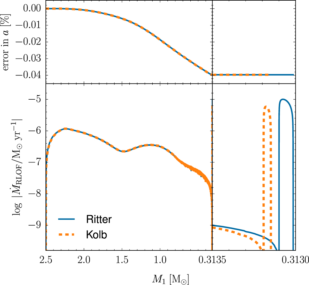
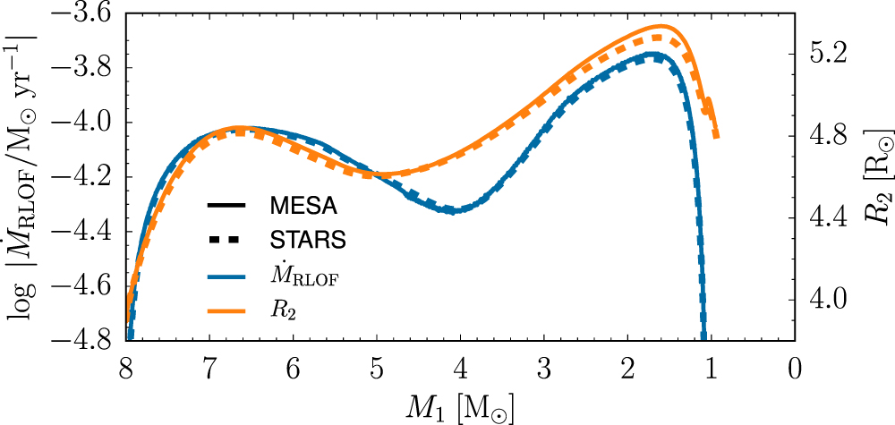
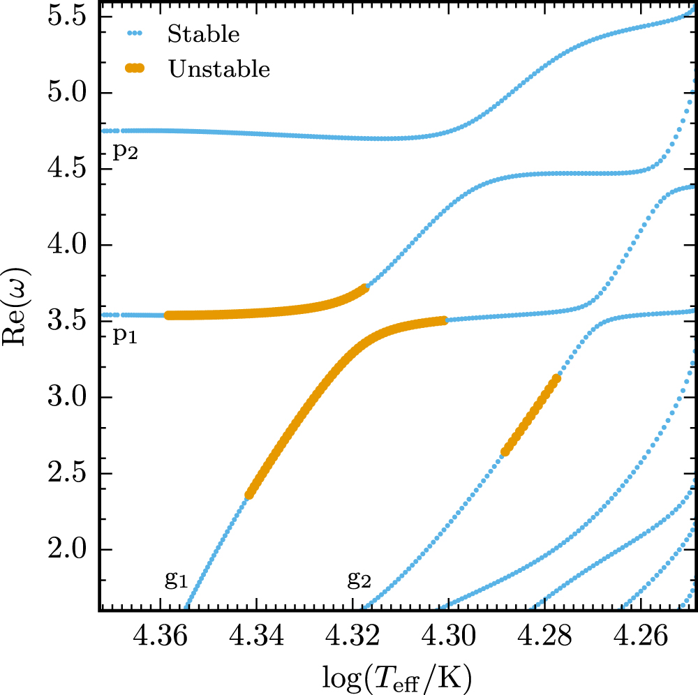
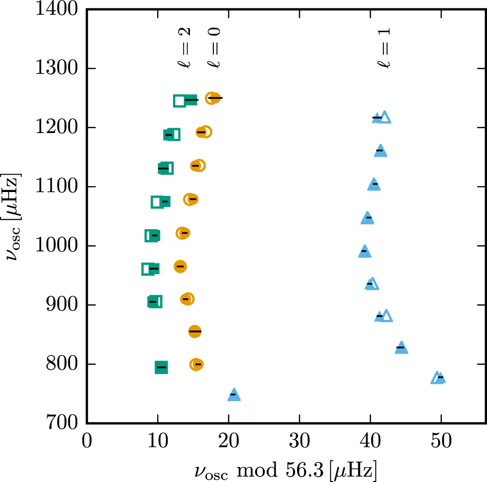
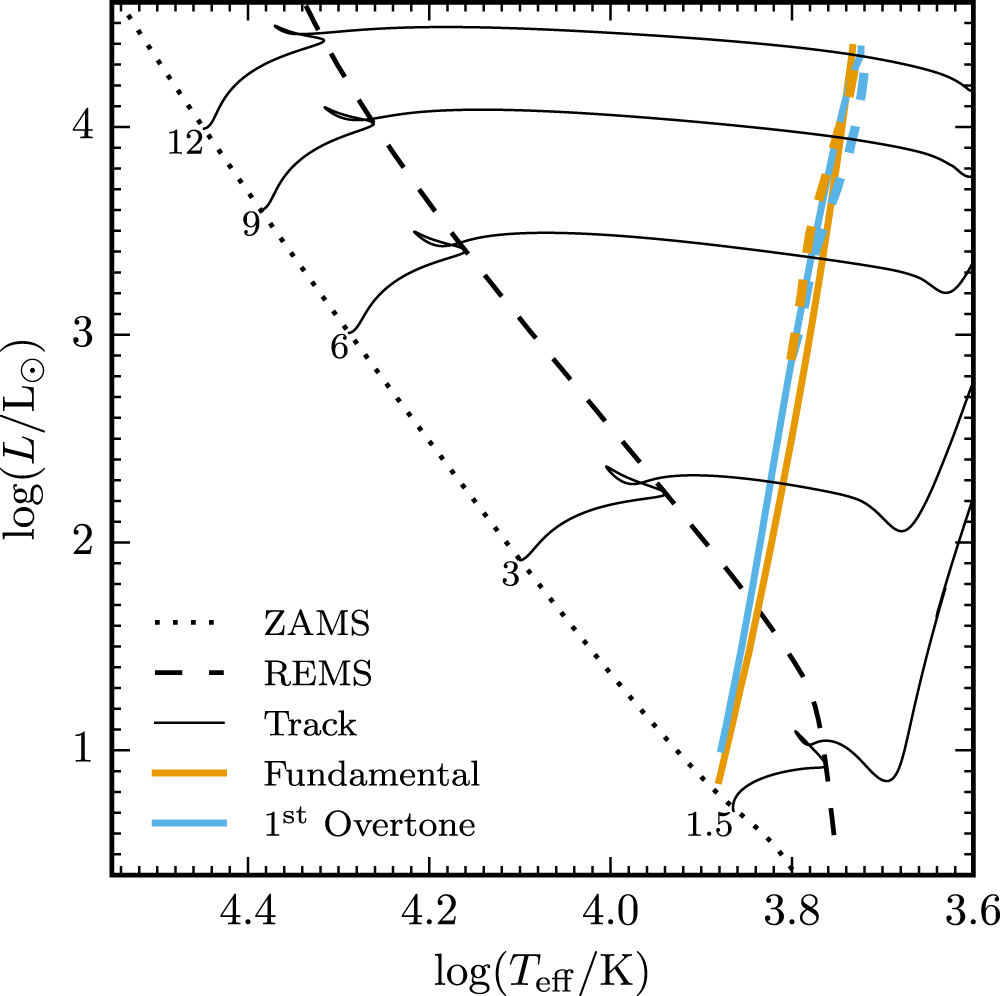
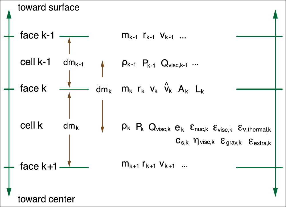
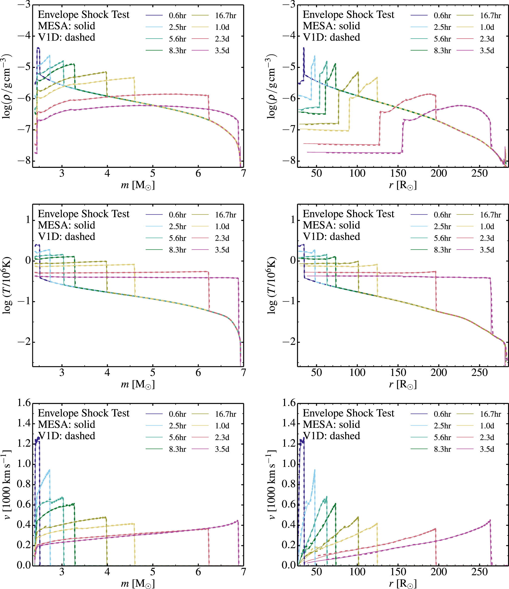
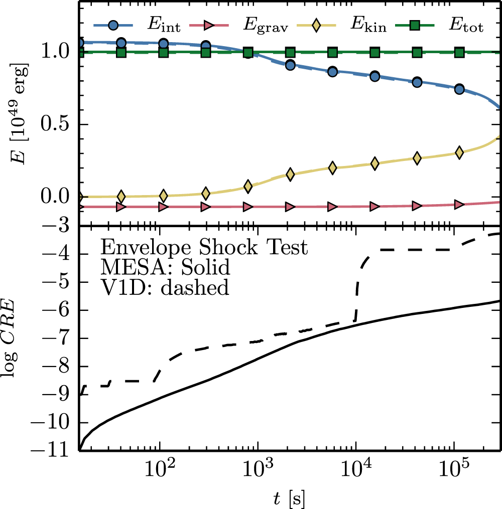
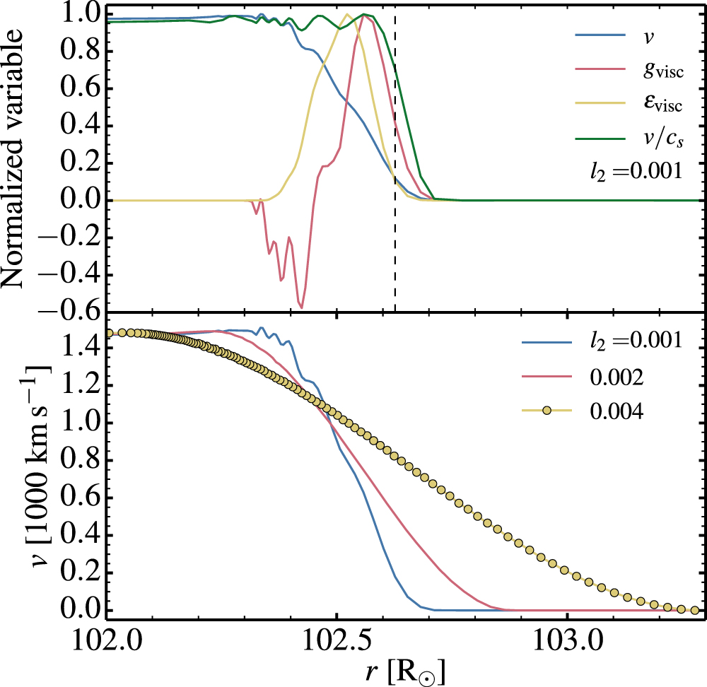
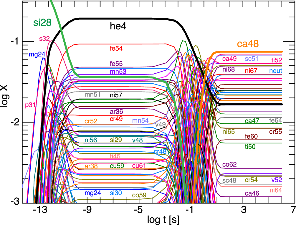
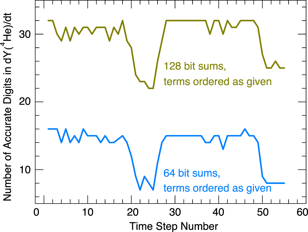
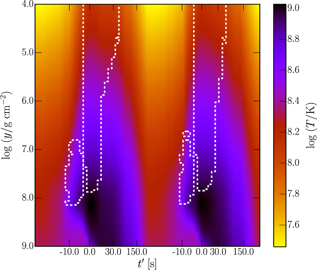
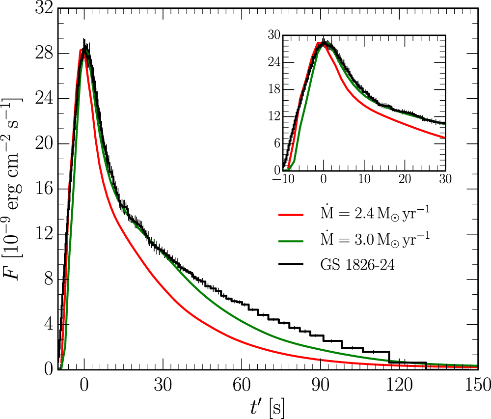
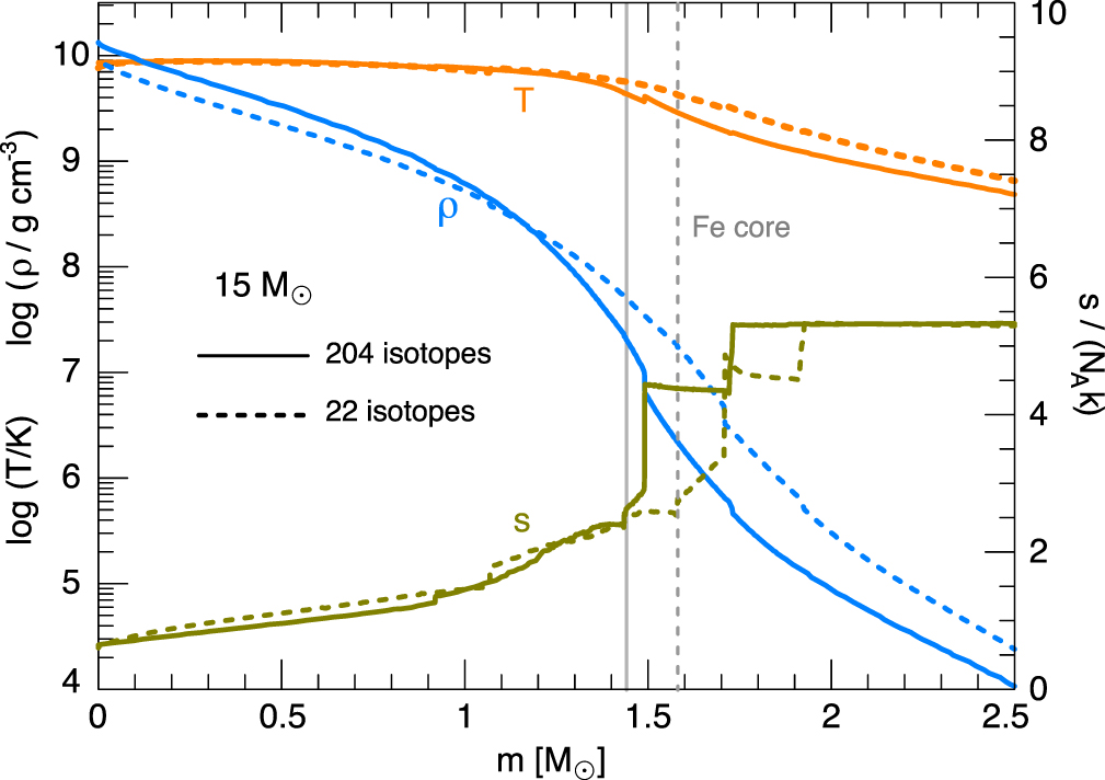
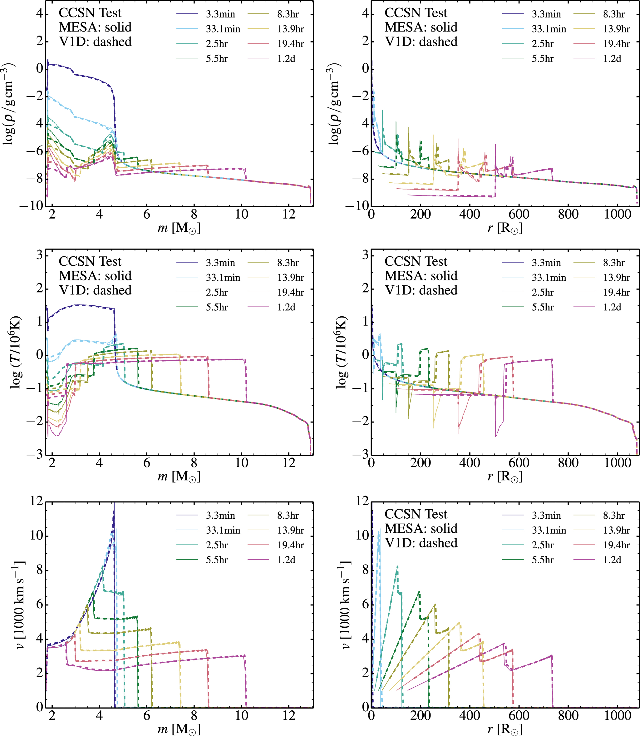
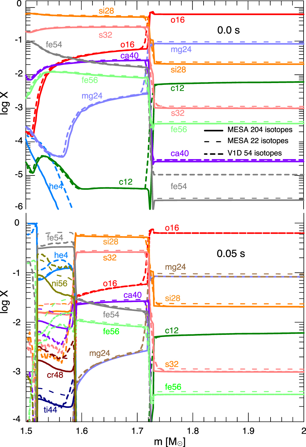
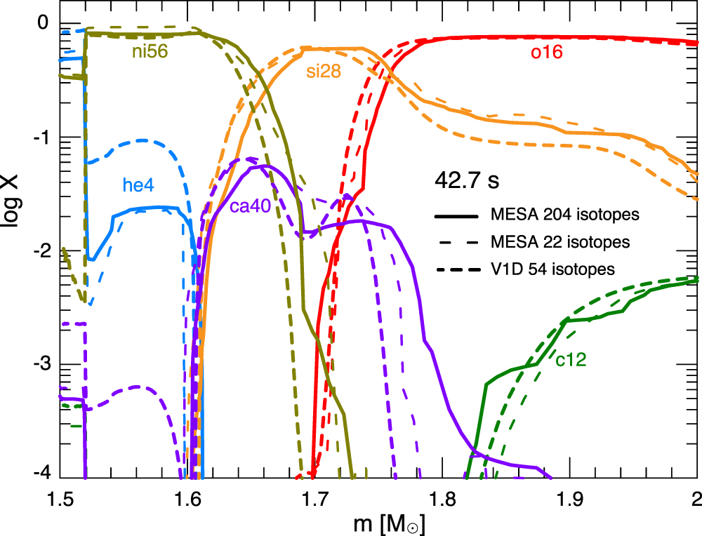
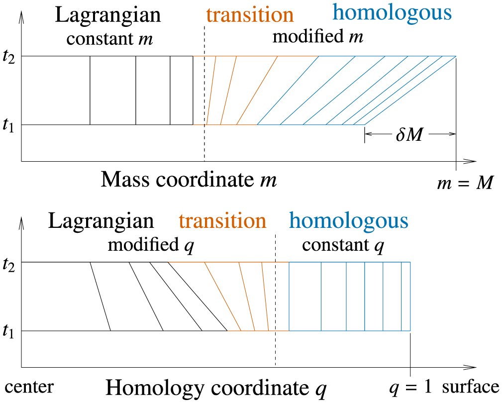
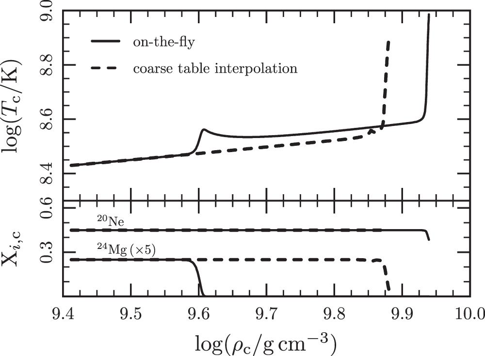
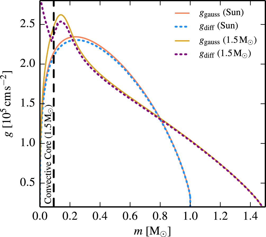
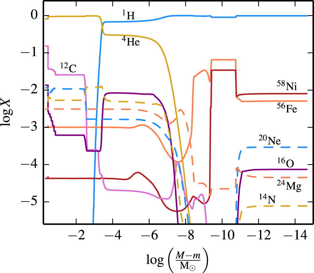