


ABSTRACT
This paper is the second in a two-part study devoted to developing tools for a systematic classification of the wide variety of atmospheric waves expected on slowly rotating planets with atmospheric superrotation. Starting with the primitive equations for a cyclostrophic regime, we have deduced the analytical solution for the possible waves, simultaneously including the effect of the metric terms for the centrifugal force and the meridional shear of the background wind. In those cases where the conditions for the method of the multiple scales in height are met, these wave solutions are also valid when vertical shear of the background wind is present. A total of six types of waves have been found and their properties were characterized in terms of the corresponding dispersion relations and wave structures. In this second part, we study the waves' solutions when several atmospheric approximations are applied: Lamb, surface, and centrifugal waves. Lamb and surface waves are found to be quite similar to those in a geostrophic regime. By contrast, centrifugal waves turn out to be a special case of Rossby waves that arise in atmospheres in cyclostrophic balance. Finally, we use our results to identify the nature of the waves behind atmospheric periodicities found in polar and lower latitudes of Venus's atmosphere.
Export citation and abstract BibTeX RIS
1. INTRODUCTION
Despite the variety of wave activity seen in Venus and Titan, which are, to date, the only known examples of cyclostrophic atmospheres (Belton et al. 1976; Seiff et al. 1992; Peralta et al. 2008; Tellmann et al. 2012; Picialli et al. 2014; Lorenz et al. 2014), a systematic classification of the observed waves based on their properties and their corresponding dispersion relations has never been done even though some of these waves have been studied individually. For instance, gravity waves are probably most exhaustively explored in the case of Venus because of their interesting relation with convective activity like that occurring in the cloud layer of Venus (Leroy & Ingersoll 1995; Baker et al. 2000a, 2000b; Yamamoto 2003; McGouldrick & Toon 2008; Piccialli et al. 2014). The presence of global-scale waves of a different nature has also been investigated with direct observations in Venus (Del Genio & Rossow 1990; Rossow et al. 1990; Kouyama et al. 2012, 2013) as well as the waves predicted by different atmospheric models (Yamamoto 2001; Imamura 2006; Lebonnois et al. 2010). These global-scale waves have been usually interpreted as special cases of global-scale terrestrial analogs such as Kelvin waves (Del Genio & Rossow 1990; Smith et al. 1992; Kouyama et al. 2012), Rossby waves (Imamura 2006; Hosouchi et al. 2012; Kouyama et al. 2013), or solar tides (Peralta et al. 2012). In the first part of this work (Peralta et al. 2014), we deduced a generic dispersion relation for the acoustic and the inertia-gravity waves for a planet with a cyclostrophic atmosphere, following a procedure similar to that of Schubert & Walterscheid (1984) for Venus but additionally accounting for the centrifugal force combined with the meridional shear of the background wind. Nevertheless, the same dispersion relation can give birth to waves of different natures when we apply different atmospheric approximations, as will be demonstrated in this paper.
Both the cloud region of Venus and the low atmosphere of Titan exhibit a variety of atmospheric conditions dominated by atmospheric stability and strong winds, as determined by several space probes during their descent (Gierasch et al. 1997; Fulchignoni et al. 2005). While the troposphere and lower stratosphere of Titan are basically stable (Strobel et al. 2010), Venus's atmospheric conditions are far more varied with at least two stable layers (between 30 and 48 km, and upward of 55 km) separated by layers of instability (Kliore & Patel 1980; Gierasch 1987), while cloud tracking, together with in situ measurements by probes, has detected different wind profiles depending on the altitude and latitude range (Gierasch et al. 1997; Hueso et al. 2012). As a result, several of the classical atmospheric approximations—such as hydrostatic balance, Boussinesq, or anelasticity—can be applied globally or locally within the cloud region of Venus to study waves other than acoustic or inertia-gravity waves. Moreover, the VEGA balloons described horizontal trajectories at an altitude of about 53 km in the Venus atmosphere that lasted for about two days and proved that—except for some episodes—the vertical wind exhibits small oscillations (Sagdeev et al. 1986), validating the assumption of waves with strictly horizontal oscillations. On the other hand, stratification effectively divides the atmosphere into two distinct but coupled atmospheric layers: the troposphere, from the surface to thermal inversion at 60 km, and the middle atmosphere or mesosphere, from 60 to about 100 km (Tellmann et al. 2009). This clear separation between media of different properties at about 60 km merits a study from the point of view of surface waves; indeed, the assumption of a shallow water system on a sphere has also been used often to study the atmospheric dynamics on Venus (Iga & Matsuda 2005).
The main objective of this work is to study the atmospheric waves which arise as a solution of the perturbed primitive equations for a cyclostrophic atmosphere when different atmospheric assumptions are applied. Once deduced, we will apply the equations to Venus, obtaining the dispersion graphs for different atmospheric regions and classifying some global-scale periodicities detected along the many spatial missions exploring Venus and through ground-based observations. In Section 2, we demonstrate that all acoustic and inertia-gravity waves can be filtered out when the cyclostrophic atmosphere is in hydrostatic balance, the Boussinesq approximation is applied, and if we have a null local rate of change of the horizontal velocity divergence. Sections 3–5 are devoted to the characterization of Lamb, surface, and centrifugal waves, respectively. Finally, the classification of Venus's atmospheric periodicities and the conclusions of this work are presented in Sections 6 and 7, respectively.
2. FILTERING ACOUSTIC AND GRAVITY WAVES
It can be demonstrated that, as a result of a proper scale analysis and after applying the method of perturbations, a cyclostrophic atmosphere can be described by the following set of perturbed equations (Peralta et al. 2014):
where (u', v', w') are the wave perturbations for the three components of the wind velocity; ρ0(z) and u0(y, z0) are the atmospheric density and zonal wind in their basic states; P', ρ', and Θ' are the perturbations for pressure, density, and the natural logarithm of the potential temperature (Θ ≡ ln θ); H0 is the density scale height (defined as 1/H0 ≡ −∂ln ρ0/∂z); g is the acceleration of gravity; B is the atmospheric static stability (B ≡ ∂ln θ/∂z) with the Brunt–Väisälä frequency being  ; and the term Ψ ≡ (u0/a)tan ϕ is the centrifugal frequency which plays a role similar to the Coriolis factor in atmospheres with a geostrophic balance like the Earth. As in Paper I (Peralta et al. 2014), we apply the method of multiple scales in altitude (Boyd 1978) to study the waves, i.e., we obtain the wave solutions for a background with only horizontal shear at a given altitude, and these solutions can be used later to reconstruct the vertical structure of the wave by considering the vertical shear of the background wind (see Appendix B in Peralta et al. 2014). For this reason, in this work, we will obtain the wave solutions for only horizontal shear and leave the task of vertically reconstructing the wave to future works. As a consequence, all the wave properties can be studied except for the overall amplitude and phase factors (Boyd 1978).
Additionally, we introduced the so-called "tracer parameters" (n1, n2, n3, n4) which multiply those terms in the wave disturbance equations that are related to the most relevant assumptions for filtering waves, following the method originally suggested by J. S. A. Green (1970, unpublished lecture notes, Imperial College) and repeatedly used in the bibliography (Green 1999; Norbury & Roulstone 2002). The effect that each of these approximations has in wave filtering was studied in detail in Paper I and is summarized as follows: the hydrostatic approximation (Dw/Dt = 0) is applied when setting n4 = 0 in the vertical momentum equation (Equation (1c)) while keeping n1 = n2 = n3 = 1 in the other equations and can be demonstrated to filter high-frequency waves; on the other hand, an incompressible atmosphere (Dρ/Dt = 0) is applied when n1 = n2 = n3 = 0 and n4 = 1, which enables filtering out of the acoustic waves, while leaving a distorted form of inertia-gravity waves. If we assume that the atmosphere behaves as intrinsically anelastic (i.e., anelastic relative to the background zonal wind), then we must set n2 = n3 = 0 and n1 = n4 = 1; this filters out the acoustic waves while leaving the gravity waves practically unaltered. Finally, the assumption of an incompressible atmosphere in hydrostatic balance (n1 = n2 = n3 = n4 = 0) can be demonstrated to be equivalent to applying the Boussinesq approximation to a cyclostrophic regime in hydrostatic balance (see Appendix A), and as a result, this effective filters all acoustic waves and part of the gravity waves (Peralta et al. 2014).
Now, we proceed to demonstrate that suppressing the local rate of change of the horizontal velocity divergence allows filtering the gravity waves in a cyclostrophic atmosphere, identically to what happens in the case of a geostrophic atmosphere (Holton 2004). The assumption of a null rate for the horizontal velocity divergence is generally considered valid for processes on synoptic scales whose timescales are usually longer than for smaller ones (Thomas et al. 2012), and it is also applied when the atmosphere can be regarded as incompressible (div  = 0). For simplicity, we will assume for this demonstration that the waves produce perturbations only in the X–Z plane, so we will have ∂/∂y = 0 for all the disturbances. Applying all of the previous assumptions together (n1 = n2 = n3 = n4 = 0), the wave disturbance equations (Equations (1a)–(1e)) become

If we apply ∂/∂x to Equations (2a) and (2b) and name the horizontal divergence as Div = ∂u'/∂x, we obtain
where we have marked the material derivative of the horizontal velocity divergence (Div) with a new tracer parameter n5. If we assume that the wave disturbances have the form ![$u^{\prime} (x,z,t) = \hat u(z) \cdot \exp \left[ {i \cdot (k_x x - \omega t)} \right]$](https://content.cld.iop.org/journals/0067-0049/213/1/18/revision1/apjs497212ieqn3.gif) , we can then replace the wave disturbances by their expression in terms of amplitude and their intrinsic frequency
, we can then replace the wave disturbances by their expression in terms of amplitude and their intrinsic frequency  ,
,


Using the thermodynamic equation (Equation (4e)) to replace  in the vertical momentum equation (Equation (4c)), then dividing the horizontal momentum equations (Equations (4a) and (4b)) by kx, we get

From Equations (5a) and (5b) and defining ξ2 = 2Ψ(Ψ − du0/dy), we can solve for the wave amplitudes for zonal and meridional wind velocities:
Replacing  in Equation (5d), Equations (5c) and (5d) become
Calculating  from Equation (7b), it is possible to use Equation (7a) to obtain the following second-order equation for the amplitude of the vertical velocity component:
which admits as a solution a wave with the following dispersion relation:
If we compare Equation (9) with the dispersion relation for inertia-gravity waves (Peralta et al. 2014),
it can be seen that in the case n5 = 1, the dispersion relation (Equation (9)) yields a distorted form of inertia-gravity waves because of the hydrostatic and incompressibility approximations. From this, it is also straightforward to conclude that forcing n5 = 0 (i.e., suppressing the local rate of change of divergence) removes the waves, thus filtering all the gravity waves.
3. EXCLUSIVELY HORIZONTAL WAVES (LAMB WAVES)
We will now study the solution for waves whose oscillations are exclusively horizontal, which, in the case of Earth, are called Lamb waves. From Equations (1a) to (1e), we can obtain a modified version of the vertical momentum and continuity equations in terms of the wave amplitudes (Peralta et al. 2014):
If we set  and assume that
  ,
,
Using Equation (12a), and if no additional assumptions are made for the atmosphere (n2 = n3 = 1), we can calculate the real part of the wave amplitude in the pressure ( ) and check that it exhibits an exponential variation with height proportional to the static stability:

Now, considering again n2 = n3 = 1, we obtain from Equation (12b) the following dispersion relation:

which is identical to the one for the geostrophic case, except that here the frequency ξ replaces the Coriolis factor f. Also note that Equations (12a) and (12b) have a solution only if n2 = n3 = 1, so Lamb waves cannot exist in the cyclostrophic atmosphere if it does not behave as elastic. This implies that, analogously to what happens in a geostrophic atmosphere, in this case, the Lamb waves are also a type of acoustic wave.
The dispersion graph based on Equation (14) for the Lamb waves in the case of Venus is displayed in Figure 1. Two limiting cases can be considered: for very small horizontal wavelengths (i.e., very large kx) the Lamb waves have intrinsic phase and group velocities that match the speed of sound relative to the background wind, while in the opposite case of very large horizontal wavelengths (i.e., very small kx) the intrinsic phase velocity coincides with that of pure inertial waves (Peralta et al. 2014) and the intrinsic group velocity is null:


Figure 1. Dispersion graph for atmospheric waves of Venus at a latitude of 45º and an altitude of 60 km. The acoustic, gravity, inertial, Lamb, surface, and centrifugal waves are shown in red, blue, orange, pink, green, and blue, respectively, with several vertical wavelengths marked with different line styles for the acoustic, gravity, and centrifugal waves. The Brunt–Väisälä frequency (BV), centrifugal frequency (Ψ), and centrifugal frequency modified by the meridional shear of the background zonal wind (ξ) are marked with gray lines. Note that the centrifugal waves must have frequencies lower than ξ. The solutions for acoustic, gravity, and inertial waves were deduced by Peralta et al. (2014).
Download figure:
Standard image High-resolution image4. SURFACE WAVES
Surface waves are waves that appear at the boundary between two media or regions of the same fluid with different densities (such as, for example, an inversion layer in the atmosphere). They cannot be exclusively categorized as inertia-gravity waves as they are mechanical waves whose restoring forces can be (or combine) the buoyancy force, surface tension, or inertial forces such as Coriolis or the centrifugal force (or both). The type of restoring forces involving a surface wave strongly depends on the characteristics of the interface and/or the spatial scale of the surface wave. In the case of Venus, the stratification allows one to divide the atmosphere into two distinct regions: the troposphere, from the surface to the thermal inversion at 60 km, and the middle atmosphere or mesosphere, from 60 to about 100 km (Tellmann et al. 2009); this division between media of different properties at about 60 km is expected to enable the existence of surface waves near the interface.
When dealing with surface waves, the boundary is usually regarded as a "free surface" (i.e., the surface shape must respond to the motion within the fluid) and cannot be determined a priori, which implies that the fluid motion and the boundary shape must be calculated simultaneously for a complete solution of a free-boundary problem. The following second-order differential equation can be obtained for the wave amplitude in the vertical velocity when studying a cyclostrophic atmosphere (Peralta et al. 2014):
To simplify the procedure, we assume that the atmosphere is intrinsically anelastic (i.e., n2 = n3 = 0, hence acoustic waves are automatically filtered out), and that the fluid behaves as unstratified (B = 0) in the boundary and the surroundings. This latter assumption necessarily imposes a limitation (to be discussed later) on the ratio between the size of the surface wave and the equivalent depth. With the mentioned assumptions, the differential equation (Equation (16a)) then becomes
In order to solve this differential equation, we define the boundary conditions suitable for a problem of surface waves (see Figure 2). The boundaries constraining our system will be a rigid horizontal boundary at the ground (z = 0) and a free surface above (at z = h(x, t)). Three boundary conditions can then be defined. First, the vertical velocity must be zero at the rigid boundary (i.e., w = 0 at z = 0). Second, the two media do not separate from the common boundary and their molecules cannot travel across the boundary (i.e., w = Dh/Dt at z = h(x, t)). Third, the pressure for the two fluids must be equal at the common boundary (P1 = P2 at z = h(x, t)) and the pressure is constant above the free surface (DP1/Dt = DP2/Dt at z = h(x, t)), both implying that DP/Dt = 0 at z = h(x, t).

Figure 2. General scheme for surface waves. The boundaries are a rigid horizontal boundary at the bottom (z = 0) and a free surface at the top, at a mean altitude of z = h0, separating two media with different properties (media 1 and 2). In the presence of these waves, the altitude of the boundary is given by a wave perturbation z = h(x, t) with an amplitude  .
.
Download figure:
Standard image High-resolution imageCaution must be taken when applying the second boundary condition: for example, in the case of Venus, a convection layer exists in the 47–60 km range, and this may involve deep convective plumes and mixing of air that may violate this boundary condition (Baker et al. 2000a, 2000b). Nevertheless, the only clear indications for convective activity at the cloud tops seem to occur around the subsolar point, so the mentioned boundary condition may still be valid far from it and at the nightside of the planet. On the other hand, if a Hadley-cell circulation exists in the planet (Peralta et al. 2007; Sánchez-Lavega et al. 2008), this would additionally restrict the study of surface waves to regions other than where ascending/subsiding motions occur.
Because we want to linearize the boundary conditions, we will take into account that
Therefore, the linearized boundary conditions are
where for the third condition, we make use of the hydrostatic balance for the basic state:
If we now assume that all the disturbances have the wave form ![$u^{\prime} (x,z,t) = \hat u(z) \cdot \exp \left[ {i \cdot (k_x x - \omega t)} \right]$](https://content.cld.iop.org/journals/0067-0049/213/1/18/revision1/apjs497212ieqn12.gif) , then we obtain the following boundary conditions written as functions of the wave amplitudes,
, then we obtain the following boundary conditions written as functions of the wave amplitudes,
Now we write the boundary condition (c) in terms of only  . Going back to the modified version of the continuity equation (Equation (11b)):
we can calculate  from Equation (22), and then replace it in the boundary condition (c), thus obtaining
Considering that  (Vallis 2006), Equation (23) becomes
where we note that (n1 − n2)/H0 is a spurious term that automatically disappears when no approximations are made (i.e., when n1 = n2 = n3 = n4 = 1; see Peralta et al. 2014). Thus, we can remove it for the boundary condition (c) and finally obtain the following differential equation and boundary conditions for the surface waves:

4.1. Long Horizontal Wavelength Limit for Surface Waves
We first consider the limit cases of kx · h0 ≪ 1 and kx · H0 ≪ 1 (i.e., the horizontal scale is much higher than the vertical scale). We can then apply the hydrostatic approximation by setting n4 = 0 (Peralta et al. 2014), thus having

and Equation (26), along with these boundary conditions, has the solution
Replacing the solution (Equation (27)) in the boundary condition (b) at z = h0, we find that the disturbances for the vertical velocity and height of the free surface have a phase difference of 90º for surface waves with long horizontal wavelengths:

Moreover, inserting the solution (Equation (27)) for z = h0 in the boundary condition (c) from Equation (26b), we obtain the following dispersion relation for surface waves with long horizontal wavelengths:

The dispersion relation (Equation (29)) can also be simplified for two limit cases. In the case of long surface waves propagating in shallow water (h0 ≪ H0), we can apply a first-order Taylor expansion (e−x ≈ 1 − x) to the exponential and obtain the following dispersion relation and intrinsic horizontal phase velocity:
Returning to the case of Venus, we have that in the cloud region H0 ≈ 6380m (Seiff et al. 1985), i.e., the limit case of large surface waves in deep water (h0 ≫ H0). Then, since 1 − exp (− h0/H0) ≈ 1, the dispersion relation and horizontal phase velocity (see Figure 1) adopt the form of Poincaré waves on Earth (Cushman-Roisin 1994):
4.2. Short Horizontal Wavelength Limit for Surface Waves
We now examine the other limit case of kx · h0 ≫ 1 and kx · H0 ≫ 1, where the horizontal scale is smaller than the vertical scale. Under this condition, the hydrostatic approximation can no longer be applied (Peralta et al. 2014), thus the differential equation and boundary conditions to be solved are
This differential equation for short horizontal wavelengths has a more complex solution than the previous equation for long wavelengths:
and in those cases where  (high intrinsic phase speeds) or ξ → 0 (waves at the equator or in regions with very small zonal winds), the amplitude for the disturbances in the vertical velocity resembles that of the geostrophic case:
If we now substitute solution (33) in the boundary condition (c) of Equation (32b), we can obtain the corresponding dispersion relation:
which can be simplified by applying H0kx ≫ 1, yielding the following dispersion relation for small surface waves:
which must be solved iteratively. In the case of Venus, ξ2 ≈ 10−10s−2 (Peralta et al. 2014) and even for very small horizontal wavelengths,  . Therefore, on Venus, the dispersion relation for short surface waves (see Figure 1) coincides exactly with the one for a geostrophic case (Salby 1996):

and in the case of very large kx · h0 (on Venus, this would correspond to waves with horizontal wavelengths lower than about 50 km for h0 ≈ 60 km), we can take advantage of the fact that tanh x ≈ 1 when x ≫ 1. In this case, we obtain waves that are much slower than long waves and have the same dispersion relation as the terrestrial deep water waves (Salby 1996):

5. CENTRIFUGAL WAVES
As mentioned before, the Coriolis force plays a negligible role in the atmospheric dynamics of a cyclostrophic regime due to the slow rotation of the planet and, thus, the classical Rossby waves found in geostrophic regimes are not expected. However, we show that the cyclostrophic metric terms yield a restoring force responsible for a special type of Rossby wave which we designate as a centrifugal wave. These centrifugal waves can be demonstrated to adopt the same formulation as the geostrophic Rossby waves when observed from a frame fixed to the profile of zonal winds (see Appendix B). Nevertheless, it will be seen that geostrophic and cyclostrophic versions of the Rossby waves are not fully equivalent since the profile of zonal winds is far from a solid-body rotation in both Titan (Flasar et al. 2010) and Venus (Peralta et al. 2007; Sánchez-Lavega et al. 2008), thus implying an equivalent angular velocity (Ω≅u0/(a · cos ϕ)) without a constant value at all latitudes and, thus, a different validity of the β-plane approximation.
In this section, we deduce the corresponding dispersion relation for centrifugal waves but focusing particularly on the case of Venus, hence implying caution when applying the dispersion relation for other planets with a cyclostrophic atmosphere. The specific assumptions suitable for the case of Venus are (1) the static stability is approximately constant with altitude (dB/dz≅0) in the region of interest, and (2) the meridional shear of the background zonal wind is negligible in the region where the β-plane approximation is valid for the centrifugal frequency Ψ.
5.1. Dispersion Relation for Centrifugal Waves
In order to describe centrifugal waves, we first filter out the acoustic and internal gravity waves. For a global scale, any atmosphere can be considered to be in hydrostatic balance and it is reasonable to apply the Boussinesq approximation (thus allowing one to filter the acoustic waves, as this approximation implies regarding the atmosphere as incompressible). Given the number of atmospheric approximations made in this case, we take advantage of the simpler form for the system of equations and consider the more general case of waves propagating in any direction (not just X–Z). The perturbed wave equations thus become (see Appendix A for a demonstration)
To simplify the notation of this section, we again use the material derivative D/Dt ≡ ∂/∂t + u0∂/∂x. For simplicity, we assume that the static stability is approximately constant with altitude dB/dz≅0. For instance, this is locally fulfilled in the Venus atmosphere (Tellmann et al. 2009).
Similar to the Coriolis factor on a rapidly rotating planet, we consider that the β-plane approximation is valid for the centrifugal frequency (i.e., Ψ ≈ Ψ0 + β · y). In fact, making use of our updated latitude–height profile for the zonal wind at the cloud region (Peralta et al. 2014), it can be checked that the β-plane approximation is fulfilled in the Venus atmosphere equatorward of midlatitudes with β < 0 (see Figure 3). Moreover, since between the equator and midlatitudes of Venus, the zonal wind is nearly constant with increasing latitude (Peralta et al. 2007; Sánchez-Lavega et al. 2008), we can further assume that the meridional shear of the wind can be neglected |∂u0/∂y|≅0 in the region where the β-plane approximation is applicable.
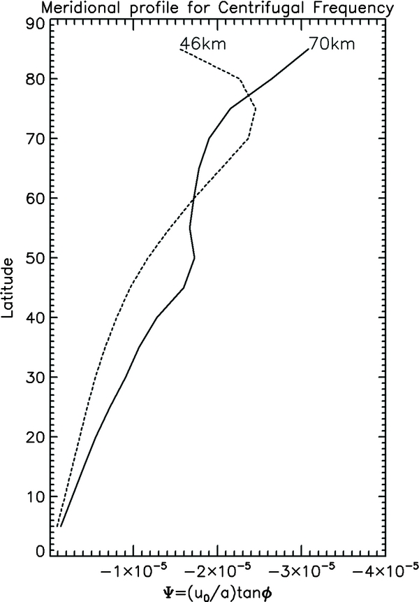
Figure 3. Meridional profile of the centrifugal frequency Ψ at two different altitudes, as obtained with an updated latitude–height zonal wind profile for the cloud region of Venus (Peralta et al. 2014). Observe that, equatorward of 45º, the centrifugal frequency is properly described with the β-plane approximation.
Download figure:
Standard image High-resolution imageIf we apply ∂/∂z to Equation (39e), we can combine Equations (39d) and ∂/∂z (Equation (39e)) to reduce the set to four equations:

Applying ∂/∂z and D/Dt to Equation (40c), we can also combine Equations (40c) and (40d) to obtain only three equations:
Now we remove the gravity waves by suppressing the local rate of change of the horizontal velocity divergence, as demonstrated in Section 2. To carry out this, we need to calculate ∂/∂x (41a)+∂/∂y (Equation (41b)) and ∂/∂y (Equation (41a))–∂/∂x (Equation (41b)), and considering that D/Dt(∂u'/∂x + ∂v'/∂y) = 0, we obtain
Applying D/Dt to Equation (42a) and multiplying Equation (42b) by Ψ, we have
In Equation (43a), we can replace Du'/Dt by its expression given by Equation (40a):

Since D/Dt(∂u'/∂y) = ∂/∂y(Du'/Dt), we can again use Equation (40a) in Equation (44a) to obtain
and combining both equations to remove the term Ψ · D/Dt(∂u'/∂y − ∂v'/∂x), we arrive at the following single equation:
Then, we replace the term 2Ψ2(∂u'/∂x + ∂v'/∂y) in Equation (46) using Equation (41c), thus obtaining an expression in terms of only the pressure and meridional velocity disturbances:
Using Equation (40a), we can also replace 2Ψ · v' and obtain
Finally, as the atmosphere can be regarded as being in approximately cyclostrophic balance, it is reasonable to assume that  and |Du'/Dt| ≪ |Ψ · v'|, so Equation (48) finally becomes in terms of a single variable
We can linearize the different terms of Equation (49), assuming for the perturbations, the form ![${{P^{\prime} } /{\rho _0 }} \propto {{\hat P} / {\rho _0 }} \cdot \exp \left[ {i \cdot \left({k_x x + k_y y + mz - \omega t} \right)} \right]$](https://content.cld.iop.org/journals/0067-0049/213/1/18/revision1/apjs497212ieqn19.gif) ,
,
thus, obtaining the following equation in terms of the wave amplitude:
and, from the imaginary part of Equation (51), we obtain the following dispersion relation for the centrifugal waves:
Upon comparison with the dispersion relation for geostrophic Rossby waves below (Salby 1996), it can be seen that the main differences are that we have 2Ψ2 instead of f2, which is the result of having 2Ψ in the meridional momentum equation (Equation (40b)) instead of a single Ψ:
We also see that the density scale height (H0) has disappeared as a result of filtering the acoustic and gravity waves by regarding the atmosphere as incompressible. In the case of Earth, the anelastic approximation is typically used for the derivation of Rossby waves.
Equation (52b) also shows that the centrifugal waves are dispersive and do not appear as pairs of westward and eastward waves relative to the background wind, but their sense depends on the sign of β (in the case of Venus, this is negative for almost all latitudes except poleward of 75º at lower heights). This also implies that—except at polar latitudes where β can change its sign—the phase of the centrifugal waves moves in the opposite sense of the superrotation: on Venus, it moves eastward relative to the mean flow, while in the case of the Rossby waves on Earth, the phase moves westward (relative to a mean flow, if present). The range for possible wavelengths and intrinsic phase velocities can be examined in the dispersion graph already shown (see Figure 1). If we examine the limit case of centrifugal waves with short wavelengths, then  , and the dispersion relation can be expressed as

In this case, we can see that, relative to the background zonal wind, for the centrifugal waves, the group velocity is of the opposite sign of the phase velocity, identical to what happens with Rossby waves on Earth,
6. CLASSIFICATION OF ATMOSPHERIC PERIODICITIES
Up until this point, we have successfully derived the dispersion relation for up to six types of atmospheric waves that can propagate in a planet whose atmosphere is governed by a cyclostrophic regime: acoustic, inertia-gravity, Lamb, surface, and centrifugal waves. These dispersion relations easily permit a classification of the atmospheric waves apparent in observations whenever we can measure some of their parameters: for instance, we can use a dispersion graph (see Figure 1) to identify waves once the horizontal wavelength and intrinsic phase velocity are obtained, as we already did in Paper I for mesoscale waves (Peralta et al. 2014). Unfortunately, actual observational techniques do not yet allow observing wave packets apparent in exoplanet clouds or carrying out limb soundings in search of vertical wave oscillations.
The first evidence of atmospheric waves in exoplanets will undoubtedly come through the identification of periodicities arising from planetary-scale waves affecting different physical parameters such as the thermal emission of a planet or the albedo of clouds. In fact, Demory et al. (2013) recently provided promising results of cloud contrasts on an exoplanet. In the case of Venus, a wide variety of periodicities has been detected with observations at different wavelengths through their effects on upper cloud patterns for reflected sunlight (Del Genio & Rossow 1990; Hosouchi et al. 2012), thermal emission (Apt & Leung 1982), and also winds (Rossow et al. 1990; Kouyama et al. 2013; Khatuntsev et al. 2013). The wave period T is given by the expression
where λx is the horizontal wavelength, u0 is the background zonal wind, and  is the intrinsic frequency for each type of atmospheric wave. Using in Equation (56) the corresponding dispersion relation
  for the waves deduced in this work, we can display a dispersion graph similar to Figure 1 but displaying observed periods against different values of horizontal wavelength (see Figure 4). Note that, in most cases, for a single period, several combinations of horizontal intrinsic phase velocity and wavelength are possible. Low-latitude periodicities detected on the dayside cloud brightness distribution (Del Genio & Rossow 1990), infrared absorption lines (Hosouchi et al. 2012), and on the zonal winds (Kouyama et al. 2013) are displayed in the top panels of Figure 4, while periodicities identified in thermal emission at polar latitudes (Apt & Leung 1982) are shown in the lower panels.

Figure 4. Dispersion graphs for periodicities detected in the Venus atmosphere at a height of about 60 km and latitudes of 20º (panels above) and 70º (panels below). The absolute periods for westward and eastward acoustic, gravity, inertial, Lamb, and centrifugal waves are shown in red, blue, orange, pink, and blue, respectively, with several vertical wavelengths marked with different line styles for the acoustic, gravity, and centrifugal waves. The reference value u0/λx (see Equation (60)) is displayed with a thick black continuous line, and values for the background zonal wind have been taken from our reference atmosphere (Peralta et al. 2014). The maximum value possible for the horizontal wavelength at each latitude is shown with the gray area. Finally, the following periodicities (given in days) are displayed with gray dotted lines for classification: 3.94, 4.0, 4.73, 5.03 (Del Genio & Rossow 1990), 3.5, 4.9, 8.4 (Hosouchi et al. 2012), 2.9, 5.3 (Apt & Leung 1982), and 255 days (Kouyama et al. 2013).
Download figure:
Standard image High-resolution image
We can extract several conclusions from our dispersion graphs. For periodicities detected at low latitudes, (1) periods higher than four days can only correspond to waves propagating eastward—in this case, centrifugal or inertia-gravity waves—while lower periods can correspond to waves propagating in both senses, (2) the long period of 255 days detected on the winds by Kouyama et al. (2013) corresponds to a global-scale centrifugal wave propagating eastward with a horizontal wavelength slightly lower than 30000 km. On the other hand, for periodicities at polar latitudes obtained from the thermal emission during the Pioneer Venus mission (Apt & Leung 1982), we are dealing with eastward gravity waves.
7. CONCLUSIONS
This is the second paper in a two-part work devoted to studying the wide variety of waves that are possible in a planet with a cyclostrophic atmosphere behaving as an adiabatic ideal gas and with a background zonal wind that varies both meridionally and vertically (Tellmann et al. 2009). Provided that the method of the multiple scales in height is applicable (Peralta et al. 2014), we studied the general properties of the atmospheric waves by solving the problem at a given height with only horizontal shear of the wind. In Paper I, a generic dispersion relation was analytically deduced for the acoustic and inertia-gravity waves. We also studied how waves are filtered when applying the classical atmospheric approximations and applied the resulting dispersion relations to classifying mesoscale waves on Venus (Peralta et al. 2014). In this second paper, we have deduced for the first time the dispersion relations for the Lamb, surface, and centrifugal waves in a cyclostrophic regime, applying all of the results to classifying global periodicities on Venus.
The Lamb waves are shown to be the solution for horizontally propagating waves, and their corresponding dispersion relation resembles that of a geostrophic analog except that the Coriolis factor is replaced by the centrifugal frequency modified by the meridional shear of the wind. Identical to the case of Earth, the Lamb waves are of an acoustic nature with high phase velocities and they can be filtered out when the atmosphere behaves anelastically relative to the background zonal wind.
The dispersion relation for surface waves has also been deduced for two limit cases: short and large waves, with the latter subdivided into deep and shallow water situations. In all cases, the wave perturbation that affects the vertical velocity is found to be phase-shifted 90º relative to the perturbed height of the free surface. On the other hand, large-scale waves in deep water and short-wavelength surface waves have a dispersion relation quite similar to the geostrophic cases.
A new type of Rossby wave for cyclostrophic regimes (here called centrifugal waves) has been found under the assumptions of hydrostatic balance, Boussinesq approximation, negligible meridional shear of the background zonal wind, and with the centrifugal frequency following a β-plane approximation. The metric terms from the cyclostrophic regime act as a restoring force in this case, and they can be regarded as equivalent to geostrophic Rossby waves when a profile of zonal winds with solid-body rotation is applicable. The centrifugal waves move eastward instead of westward in the case of Venus due to the sense of atmospheric superrotation.
Finally, we used the dispersion relations for acoustic, inertia-gravity, Lamb, and centrifugal waves to derive an expression for the absolute wave period. The results were used in dispersion graphs to classify the wide variety of periodicities found in the atmosphere of Venus at equatorial and polar latitudes. Most of the periodicities are found to fit with inertia-gravity waves, while longer periods (typically more than four days) must correspond to waves propagating only eastward. The low-latitude period of about 255 days detected on the winds by Kouyama et al. (2013) corresponds to a global-scale centrifugal wave with a horizontal wavelength slightly lower than 30000 km. Polar periodicities found from thermal emission (Apt & Leung 1982) correspond to eastward gravity waves.
The analytical dispersion relations obtained in this work are expected to contribute to the general knowledge of the atmospheric waves in slowly rotating planets with a cyclostrophic regime and atmospheric superrotation and to help in future studies by providing new tools with which to predict not only the properties of waves but also their role in the source, dissipation, and transportation of energy and momentum. In addition, our equations have allowed us to obtain dispersion graphs for different regions of Venus's atmosphere which will be useful for classifying waves that have been identified in the many space missions that have explored Venus, an important task yet to be extended to Titan and exoplanets. The derivation of the atmospheric waves that arise as solutions in the equatorial region of cyclostrophic regimes (namely, mixed and Kelvin waves) seems to be the natural continuation of this work and will be addressed in a forthcoming article.
J. Peralta acknowledges support from the Portuguese Fundação para a Ciência e a Tecnologia (FCT, grant reference: SFRH/BPD/63036/2009), from the Spanish MICINN for funding support through the CONSOLIDER program "ASTROMOL" CSD2009-00038, and also funding through project AYA2011-23552. J.P. and D.L. acknowledge FCT funding through project grants POCI/CTE-AST/110702/2009, the Pessoa-PHC programme, and project PEst-OE/FIS/UI2751/2011. A.P. acknowledges funding from the European Union Seventh Framework Programme (FP7/2007-2013) under grant agreement No. 246556. The authors are very grateful for the invaluable revision carried out by the anonymous reviewer.
APPENDIX A: WAVE EQUATIONS FOR A CYCLOSTROPHIC ATMOSPHERE UNDER HYDROSTATIC BALANCE AND THE BOUSSINESQ APPROXIMATION
In the Boussinesq approximation, the density is replaced by a mean value (ρ0) that is constant everywhere except in the buoyancy term in the vertical momentum equation (Holton 2004). If we apply this approximation along with assuming that the atmosphere is in hydrostatic balance, we will have the following system of primitive equations:


where we have considered that the atmosphere is an ideal gas with adiabatic motions. The variables (u, v, w) are the three components of the wind velocity; P, ρ, T, and Θ are the atmospheric pressure, density, temperature, and natural logarithm of the potential temperature; and R is the constant for the gases. Now, we assume that every variable can be divided into two parts: a basic state and a local deviation from the basic state called perturbation or disturbance. The basic states or mean values of the variables should satisfy the governing equations themselves and the disturbances should be small enough to neglect cross terms that are products of perturbations. In this case, the disturbances for each atmospheric parameter will be
where we have regarded the atmosphere to be at rest except for a zonal background wind that depends on the latitude, i.e., u0 = u0(y), v0 = w0 = 0 (Peralta et al. 2007; Hueso et al. 2012). Introducing perturbations (Equation (A2)) in Equations (A1a)–(A1f), neglecting all terms containing products of perturbations, and defining a centrifugal frequency as Ψ ≡ (u0/a)tan ϕ,
As a first step, we combine the equation of the ideal gases (Equation (A3f)) and the vertical momentum equation (Equation (A3c)) to get rid of the density. Taking into account that,
We then have
Now, manipulating the Poisson's equation for the basic state, we can obtain the following expression:
Replacing ∂ln ρ0/∂z in Equation (A5a) and considering that the stability is defined as B ≡ ∂ln θ/∂z, the vertical momentum and ideal gas equations become
Using the hydrostatic balance again,

Joining all the terms multiplied by the acceleration of gravity in Equation (A8a) and making use of Equation (A8b), we arrive at the following expression for the vertical momentum equation:
Then, dividing Poisson's equations for disturbed and undisturbed states and operating,
Taking into account that ln (1 + x)≅x when x ≪ 1, we can modify Equation (A9) and obtain
Considering that Θ ≡ ln θ, we can demonstrate that Θ'≅θ'/θ0 by again applying ln (1 + x)≅x when x ≪ 1:
and we obtain for the vertical momentum equation:
As a last step, remembering that B ≡ ∂ln θ/∂z = ∂Θ0/∂z, we introduce the stability in the thermodynamic equation (Equation (A3e)) and we finally obtain the following set of equations for the wave disturbances:

thus demonstrating that applying the Boussinesq approximation with hydrostatic balance allows one to obtain the same set of equations as when we rotate the local frame of coordinates to have the Z-axis with the same direction as the sum of the centrifugal and gravitation forces as well as apply hydrostatic balance and an incompressible atmosphere (see Section 2).
APPENDIX B: ROSSBY WAVES FOR A FRAME FIXED TO THE SUPERROTATING WINDS IN A CYCLOSTROPHIC ATMOSPHERE
The aim of this appendix is to demonstrate that the centrifugal waves are a new type of Rossby waves in cyclostrophic regimes and that they can be regarded as locally equivalent to the classical Rossby waves when observed relative to a frame fixed on the superrotating winds. As a result of applying a proper scale analysis for such a frame, we obtain the following system of equations (for details, see Peralta et al. 2014):
which corresponds to an atmosphere that is approximately in geostrophic balance instead of cyclostrophic balance. To linearize the equations, we assume that every field variable can be divided into two parts (a basic state and a local deviation from the basic state called perturbation or disturbance):
where we have regarded the atmosphere to be at rest in its basic state. Inserting these equations into Equations (B1a)–(B1e), neglecting all terms containing products of perturbations, and applying hydrostatic balance and the Boussinesq approximation, we obtain (see details of the procedure in Peralta et al. 2014)
Despite the resemblances to the equations for the geostrophic case, this Coriolis factor is equivalent to the classical one only if the superrotating winds fit a solid-body profile, which is not valid in the case of Venus (Peralta et al. 2007; Sánchez-Lavega et al. 2008). If we consider that Ω≅u0/(a · cos ϕ) is not a function of latitude (with u0 being the background zonal wind where the frame is fixed), we can recover the definition of centrifugal frequency and obtain that f = 2Ωsin ϕ = 2Ψ. Replacing,
If we apply ∂/∂z to Equation (B4e), we can combine Equations (B4d) and (B4e) to have only four equations:

Now applying ∂/∂z and ∂/∂t to Equation (B5c), we can also combine Equations (B5c) and (B5d) to have only three equations:

Now we remove the gravity waves by suppressing the local rate of change of the horizontal velocity divergence, as it was demonstrated in Section 2. Before performing this, we will consider that we can apply the β-plane approximation between the equator and midlatitudes to this Coriolis factor, which seems correct since we have f ≈ f0 + βf · y = 2Ψ0 + 2β · y, and for the centrifugal frequency Ψ ≈ Ψ0 + β · y (with β < 0; see Figure 3). Calculating ∂/∂x (Equation (B6a))+∂/∂y (Equation (B6b)) and ∂/∂y (Equation (B6a))−∂/∂x (Equation (B6b)), and considering that ∂/∂t(∂u'/∂x + ∂v'/∂y) = 0, we obtain
Applying ∂/∂t to Equation (B7a) and multiplying Equation (B7b) by f, we have
and subtracting both equations to get rid of f · ∂/∂t(∂u'/∂y − ∂v'/∂x), we arrive at the following single equation after manipulating the terms:
We now replace the term f2(∂u'/∂x + ∂v'/∂y) in Equation (B9) using Equation (B6c):
Using Equation (B4a), we can also replace f · v' and obtain
Finally, as the atmosphere in this case was regarded as approximately in geostrophic balance, it is reasonable to assume that  and |∂u'/∂t| ≪ |f · v'|, so Equation (B11) finally becomes, in terms of a single variable,
If we assume that the perturbations are due to waves with the form ![${{P^{\prime} } / {\rho _0 }} \propto {{\hat P} / {\rho _0 }} \cdot \exp [ {i \cdot ({k_x x + k_y y + mz - \omega t})} ]$](https://content.cld.iop.org/journals/0067-0049/213/1/18/revision1/apjs497212ieqn24.gif) , we can linearize the different terms of Equation (B12),
, we can linearize the different terms of Equation (B12),
thus obtaining the following equation in terms of the wave amplitudes:
and we obtain the following dispersion relation for the Rossby waves from Equation (B14):
Considering Equation (B15b) and βf = 2β (where β is the slope for the centrifugal frequency), we see that the Rossby waves that arise in a system of coordinates fixed to the zonal background wind move eastward with a phase velocity matching the intrinsic phase velocity for the centrifugal waves:

hence confirming that the centrifugal waves observed for a frame fixed to the surface of the planet are equivalent to the Rossby waves arising for a frame fixed to the mean zonal flow of the atmosphere when we have the bulk atmosphere following a solid-body rotation.