


ABSTRACT
We describe the design and data analysis of the DEEP2 Galaxy Redshift Survey, the densest and largest high-precision redshift survey of galaxies at z ∼ 1 completed to date. The survey was designed to conduct a comprehensive census of massive galaxies, their properties, environments, and large-scale structure down to absolute magnitude MB = −20 at z ∼ 1 via ∼90 nights of observation on the Keck telescope. The survey covers an area of 2.8 deg2 divided into four separate fields observed to a limiting apparent magnitude of RAB = 24.1. Objects with z ≲ 0.7 are readily identifiable using BRI photometry and rejected in three of the four DEEP2 fields, allowing galaxies with z > 0.7 to be targeted ∼2.5 times more efficiently than in a purely magnitude-limited sample. Approximately 60% of eligible targets are chosen for spectroscopy, yielding nearly 53,000 spectra and more than 38,000 reliable redshift measurements. Most of the targets that fail to yield secure redshifts are blue objects that lie beyond z ∼ 1.45, where the [O ii] 3727 Å doublet lies in the infrared. The DEIMOS 1200 line mm−1 grating used for the survey delivers high spectral resolution (R ∼ 6000), accurate and secure redshifts, and unique internal kinematic information. Extensive ancillary data are available in the DEEP2 fields, particularly in the Extended Groth Strip, which has evolved into one of the richest multiwavelength regions on the sky. This paper is intended as a handbook for users of the DEEP2 Data Release 4, which includes all DEEP2 spectra and redshifts, as well as for the DEEP2 DEIMOS data reduction pipelines. Extensive details are provided on object selection, mask design, biases in target selection and redshift measurements, the spec2d two-dimensional data-reduction pipeline, the spec1d automated redshift pipeline, and the zspec visual redshift verification process, along with examples of instrumental signatures or other artifacts that in some cases remain after data reduction. Redshift errors and catastrophic failure rates are assessed through more than 2000 objects with duplicate observations. Sky subtraction is essentially photon-limited even under bright OH sky lines; we describe the strategies that permitted this, based on high image stability, accurate wavelength solutions, and powerful B-spline modeling methods. We also investigate the impact of targets that appear to be single objects in ground-based targeting imaging but prove to be composite in Hubble Space Telescope data; they constitute several percent of targets at z ∼ 1, approaching ∼5%–10% at z > 1.5. Summary data are given that demonstrate the superiority of DEEP2 over other deep high-precision redshift surveys at z ∼ 1 in terms of redshift accuracy, sample number density, and amount of spectral information. We also provide an overview of the scientific highlights of the DEEP2 survey thus far.
Export citation and abstract BibTeX RIS
1. INTRODUCTION
Spectroscopic redshift surveys have been a major gateway to understanding galaxy evolution. By locating each galaxy in both space and time, they provide the raw material for compiling a census of galaxy properties as a function of cosmic epoch and position in the cosmic web. Clustering measures derived from redshift surveys of sufficiently large volume—such as the correlation function, ξ(rp, Π) diagram, and measures of the local overdensity of galaxies—probe the gravitational growth of structure. Pair counts contain information on merger rates, while satellite motions probe dark-halo masses and dynamics. When the galaxy sampling is sufficiently dense, groups of galaxies become well defined and allow the estimation of the number density of groups (constraining cosmology), as well as the determination of the environments in which individual galaxies are found. The spectra themselves can reveal a wealth of detail on emission-line strengths, stellar populations, star-formation rates, active galactic nucleus (AGN) activity, gas and stellar metallicities, internal motions, and dynamical masses. Finally, spectroscopic redshifts provide the fundamental data needed for calibrating photometric redshifts, which are the only way to estimate distances for the hundreds of thousands of fainter galaxies that are beyond the reach of current redshift surveys.
Pioneering low-redshift surveys out to z ∼ 0.2, such as the Sloan Digital Sky Survey (SDSS; York et al. 2000; Abazajian et al. 2003) and the Two Degree Field Survey (2dF; Colless et al. 2001) have demonstrated the value of mammoth samples of galaxies containing hundreds of thousands of objects. Huge samples enable finer slicing in redshift and galaxy-parameter space, reveal rare phases of galactic evolution, and provide sufficient weight to measure statistical scatter about the various galactic scaling laws.
Redshift surveys of more distant galaxies at z ∼ 1 progressed more slowly, primarily as they have targeted galaxies more than 100 times fainter than SDSS or 2dF. The first substantial surveys were conducted in the 1990s, measuring redshifts of several hundred objects at intermediate redshift; e.g., the LDSS survey (Colless et al. 1990), the ESO-Sculptor Survey (Bellanger et al. 1995; Arnouts et al. 1997), the CNOC and CNOC2 surveys (Yee et al. 1996, 2000), and the Hawaii Deep Fields Survey (Cowie et al. 1996).
Surveys of even more distant galaxies began taking shape at roughly the same time. The pioneering Canada–France Redshift Survey (CFRS; Lilly et al. 1995) garnered ∼600 redshifts and was the first to provide a dense, statistical sample of galaxies out to z ∼ 1. Though conducted with only a 3.6 m diameter telescope, it had a fairly deep magnitude limit of IAB = 22.5 and yielded a median redshift of z = 0.56. Augmented by Hubble imaging, it established landmark norms for the luminosities and sizes of galaxies and the star-formation history of the universe to z ∼ 1.
The LRIS multi-object spectrograph on the Keck telescopes enabled a variety of even deeper surveys. Cowie and collaborators (Cowie et al. 1996) used roughly 400 redshifts down to I ∼ 23 in the Hawaii Deep Fields to elucidate the phenomenon of "downsizing," that the peak of star formation occurred first in the most massive galaxies and swept down later to smaller galaxies. This concept has since become central to understanding galaxy evolution. Later surveys by the same group have probed the nature of distant X-ray sources (e.g., Barger et al. 2005, 2008).
The Caltech Faint Galaxy Redshift Survey (Cohen et al. 2000) exploited the Keck 10 m telescope and went roughly 1 mag fainter than CFRS (R = 23–24), assembling several hundred redshifts with median z = 0.70 in two fields (one of them containing the Hubble Deep Field-N, HDF-N). Notable discoveries included the extreme amount of clustering found even at z ∼ 1, the relatively normal morphologies of most field galaxies observed (i.e., the rarity of true peculiars and mergers), the measurement of the shape of the luminosity function to deeper magnitudes, and the exploration of the nature of distant mid-IR and radio sources (van den Bergh et al. 2000; Hogg et al. 2000; Cohen 2002).
The largest of this first generation of deep redshift surveys was DEEP1. This survey used the LRIS instrument on the Keck I telescope to obtain spectroscopy to a magnitude limit of R ∼ 24 in and around the HDF-N and the Groth Survey Strip, a 127 arcmin2 region observed with WFPC2 on Hubble Space Telescope (HST) in both I and V (Groth et al. 1994; Vogt et al. 2005). DEEP1 was conceived and executed as a pilot survey for the DEEP2 Galaxy Redshift Survey described in this paper. Over 720 redshifts were measured in total (Phillips et al. 1997; Weiner et al. 2005) having a median value of ∼0.65, and bulge and disk parameters were fitted to the Groth Strip HST images (Simard et al. 2002). Scientific highlights include an early sub-survey that helped to establish the nature of Lyman-break galaxies (Lowenthal et al. 1997), the detection of a strong color bimodality out to z ∼ 1 (Im et al. 2002; Weiner et al. 2005), the measurement of fundamental plane evolution for distant field spheroidal galaxies (Gebhardt et al. 2003), the detection of "downsizing" in the star formation rate of compact galaxies (Guzmán et al. 1997), measurements of interstellar medium (ISM) metallicity evolution to z ∼ 1 (Kobulnicky et al. 2003), an extensive analysis of selection effects on disk–galaxy radii and surface brightnesses (SBs; Simard et al. 2002), and the discovery of the prevelance of already-red bulges in typical disk galaxies at z ∼ 1 (Koo et al. 2005; Weiner et al. 2005). A distinguishing feature of DEEP1 was the use of relatively high spectral resolution (R ∼ 3000, FWHM = 3–4 Å), which resolved redshift ambiguities by splitting the [O ii] λ3727 doublet and also yielded linewidths and rotation curves. These were used to extend the Tully–Fisher (TF) relation to z ∼ 1 (Vogt et al. 1996, 1997), a strategy that was later used in the Team Keck Redshift Survey (TKRS, GOODS-N; Wirth et al. 2004) to yield an even larger sample of linewidths (Weiner et al. 2006a, 2006b).
DEEP1 was a valuable learning experience. In addition to proving the scientific value of the high spectral resolution made possible by LRIS, it confirmed that faint spectral features could be more easily seen in the dark stretches of spectrum between the OH lines. On the other hand, achieving photon-limited sky subtraction under the newly concentrated OH lines places even higher requirements on flat-fielding accuracy, wavelength calibration, and night-sky spectral modeling. Furthermore, pushing beyond the de facto redshift limit that then existed near z ∼ 1 (the so-called redshift desert) would require pursuing [O ii] λ3727 to well beyond 8000 Å. A new spectrograph on one of the largest optical telescopes would be necessary to achieve these goals.
The present paper describes the design and execution of the DEEP2 Galaxy Redshift Survey (commonly referred to as DEEP2 in the remainder of this paper), which was conducted by a collaboration of observers primarily based at UC Berkeley and UC Santa Cruz, together with astronomers from the University of Hawaii and other institutions. The survey was executed with the DEIMOS multi-object spectrograph (Faber et al. 2003) on Keck 2; aspects of the survey have previously been described in Davis et al. (2003, 2005), Coil et al. (2004b), and Willmer et al. (2006). The survey obtained roughly 53,000 spectra, coming close to the target of ∼60,000 galaxies in the original survey design.
The DEIMOS spectrograph was designed primarily to enable the DEEP2 survey, building on the lessons learned from the surveys conducted with the LRIS instrument at Keck. It differs from LRIS primarily in utilizing a larger detector array, covering a larger field of view (FOV), offering wider spectral coverage at fixed resolution, enabling better sky-subtraction due to an active flexure compensation system (FCS), and permitting the simultaneous observation of 3–4× as many objects.
DEEP2 was conceived as a legacy survey for the astronomical community, and all data are now public. The present paper is intended as a handbook for users to understand and utilize the data products in Data Release 4 (hereafter DR4), which is available at http://deep.berkeley.edu/DR4/. Brief descriptions of the data and methods are given there, but the present account is more complete and presents new details on the final data reduction techniques, redshift measurement procedures, the current generation of redshifts, and summary data tables. Additional measurements that were not part of previous DEEP2 data products are also included. All data in this paper are available in the form of FITS BINTABLE files at the DR4 Web site.
The outline of this paper is as follows. Section 2 sets forth the overarching goals and tradeoffs that determined the design of the DEEP2 survey. Section 3 summarizes some of the major scientific results so far, giving examples of how various aspects of the design have translated into specific science gains. Section 4 gives the basic DEEP2 survey parameters and field properties and describes the extensive existing ancillary data that are available in the DEEP2 fields. DEEP2 is put into context in Section 5, which compares DEEP2 to other leading z ∼ 1 surveys (VVDS-deep, VVDS-wide, zCOSMOS, and PRIMUS) using several different measures of survey size and information content.
Section 6 describes the parent galaxy photometric catalogs and selection cuts that were used to determine potential targets for DEEP2 spectroscopy. The slitmask design process is covered in Section 7, which describes the DEIMOS detector and slitmask geometry, as well as the algorithms used to place objects on masks. Section 8 is an exhaustive discussion of all known selection effects resulting from the slitmask design process, caused either by loss of objects from the initial target pool or by systematics in the rate at which we select pool objects of given properties for masks.
Sections 9 and 10 describe the spectroscopic exposures and their reduction, including detailed information on the spec2d pipeline that produces the reduced one-dimensional (1D) and two-dimensional (2D) spectra. This pipeline has been employed by many DEIMOS users; this paper provides its definitive description. The features of the DEIMOS spectrograph and spec2d pipeline that enable photon-limited sky subtraction accuracy even under the OH lines are described in the Appendix. The range in quality of DEEP2 data is discussed in Section 10, where examples of typical data, bad data, and interesting spectra are given.
Section 11 describes the redshift measurement process, including the automated spec1d redshift pipeline that produces a menu of redshift possibilities and the subsequent visual inspection process to select among them via the interactive user GUI zspec. Final results on redshift success, quality codes, completeness, biases, and redshift accuracy are also given there. Section 12 investigates the impact of multiple galaxies masquerading as single galaxies in the ground-based pcat photometry. Section 13 is a guide to DR4 and the two main data tables in this paper, which summarize the mask data and final redshifts and quality codes.
Section 14 is provided to enable correlation function measurements with DR4 data and to aid theorists who wish to make mock DEEP2 catalogs from model galaxy data. It describes a set of files being distributed along with DR4 that describe the selection and redshift success probability for a DEEP2 target as a function of location on the sky. Finally, Section 15 illustrates the properties of the DEEP2 data set via plots of numbers, colors, magnitudes, etc., as a function of redshift.
Depending on their interests, readers may wish to focus on certain sections of this paper. For instance:
- 1.Users of DEEP2 Data Release 4 data. Key sections are Section 4 (survey parameters), Section 8 (assessment of biases in targeting), Section 10.3 (presenting sample spectra), Sections 11.3 and 11.4 (redshift results and completeness), Section 13 (describing the released data tables), Section 14 (describing the released 2D selection functions), and Section 15 (describing trends in the sample with z).
- 2.Individuals interested in the design of DEEP2 and comparison to other deep surveys. Key sections are Section 2 (design goals), Section 3 (science results), Section 4 (survey parameters), Section 5 (comparison to other surveys), Section 8 (assessment of biases in targeting), Section 12 (evaluating how frequently spectroscopic targets consisted of multiple unresolved galaxies), and Section 15 (describing trends in the sample with z).
- 3.
- 4.
Throughout this paper, unless specified otherwise we utilize magnitudes on the AB system and assume a ΛCDM concordance cosmology with Ωm = 0.3, ΩΛ = 0.7, and H0 = 100 h km s−1 Mpc−1. The DR4 data tables also use these quantities.
2. CONSIDERATIONS GUIDING THE DESIGN OF THE DEEP2 SURVEY
DEEP2 was originally envisioned as a tool for simultaneously studying galaxy evolution and the growth of large-scale structure since z ∼ 1. However, while the survey was being designed it was realized that such data could also be used to constrain the nature of dark energy (i.e., its equation of state) by counting the abundance of groups and clusters as a function of velocity dispersion and redshift (Newman et al. 2002; Newman & Davis 2000, 2002; Gerke et al. 2005). This was one of the first methods proposed for studying dark energy by counting massive objects (see also Haiman et al. 2001). The distribution of clusters in velocity and redshift depends on both the growth rate of large-scale structure and on the volume element (i.e., the amount of volume per redshift interval per angular area), which are each related to fundamental cosmological parameters in predictable ways. Counting the abundance of intermediate-mass groups to high accuracy therefore became a third major goal guiding the design of DEEP2.
It was clear from the start that one of the most important DEEP2 data products would be precision counts, to be compared with various types of model predictions. Obtaining high-precision counts requires:
- 1.many galaxies,
- 2.an accurately known and simple selection function—DEEP2 is basically magnitude-limited with nearly uniform sampling on the sky and in redshift space at z > 0.75—and,
- 3.low sample (commonly referred to as "cosmic") variance.
These aims—large numbers, simple selection function, and low cosmic variance—were the central guiding principles for DEEP2. They had to be achieved, however, while using as little total telescope time as possible.
Optimizing the measurement of environment and clustering statistics played a major role in setting the sizes and shapes of the DEEP2 survey fields. Galaxy properties vary systematically with environment, and the length-scale of this influence can shed important light on the physical mechanisms causing these effects: for example, differentiating between processes associated with the parent dark matter halo of a galaxy from those that act on larger scales. Since the typical comoving radius of galaxy groups and clusters is of order ∼1 h−1 Mpc, measuring the local overdensity of other galaxies around a given object (the most common measure of environment used today) requires counting neighbors to a separation at least this large, corresponding to 1 5 at z ∼ 1. As a result, even when corrections for lost area are applied, neighbor counts become inaccurate for galaxies that are too near to survey boundaries (cf. Cooper et al. 2005); minimizing the number of lost objects in environment studies requires:
- Fields that are at least 10 times wider in each direction than the radius within which environments are measured, corresponding to a minimum dimension of ∼15' on the sky for a survey at z ∼ 1.
This restriction also ensures that fields will be well-sized for characterizing groups and clusters, in support of our third science goal.
The measurement of correlation functions drives the choice of a minimum field dimension in similar ways, as the dominant error terms on large scales increase rapidly for pair separations larger than half the minimum field dimension (e.g., Bernstein 1994). It is also necessary to survey a large volume to minimize the effects of cosmic variance on correlation function estimates. Typical values of the scale length of galaxy clustering, r0, for galaxy populations of interest are generally ≲ 5 h−1 co-moving Mpc at z ∼ 1 (Coil et al. 2004a, 2008), corresponding to an angular separation of 74. Measuring correlation functions well therefore requires:
- Contiguous volumes spanning several times r0 in one dimension, with the other two dimensions spanning many times r0.
A field size of 0 5 × 2° was accordingly selected for three out of the four DEEP2 fields, corresponding to 4 r0 by 16 r0 at z = 1. Rectangular fields rather than square fields were chosen to increase the statistical power of the sample: the opposite ends of a strip will be more statistically independent than regions closer to each other, reducing cosmic variance (Newman & Davis 2002).
Since environment measures involve the pairwise counting of objects, the statistical weight of such data increases as the square of the volume density of galaxies sampled, all other things being equal.27 Essentially all environmental studies in the Poisson-dominated regime should benefit from this scaling, including those which employ a wide variety of galaxy environment estimators, the measurement of correlation functions and cross-correlations for dilute samples or at small scales, pair counts, comparisons of group and field populations, and studies incorporating the dynamical masses of groups. The DEEP2 targeting strategy is therefore designed to obtain:
- A high number density of galaxies (or equivalently, number of objects per unit area and redshift) down to the faintest feasible magnitude limit.
However, under the constraint of finite telescope time, the need for large, densely sampled fields to enable accurate correlation function and environment measurements conflicts with the desirability of covering many independent regions on the sky to minimize (and allow assessment of) cosmic variance. The sample variance in a single large field, whose subregions are correlated due to large-scale modes of the power spectrum, will always be greater than in a larger number of widely separated fields on the sky covering the same total area. Our preferences for large field sizes but small cosmic variance are most efficiently reconciled by choosing:
- Several widely separated areas on the sky, each one of which exceeds the minimum width and length needed for correlation and environment studies.
The final choice to survey four fields was driven by cosmic variance calculations utilizing the QUICKCV code of Newman & Davis (2002)28 and by the instability of standard deviation measurements with fewer samples. Surveying multiple fields spaced well apart in R.A. also makes telescope scheduling easier.
Obtaining a dense sample of galaxies can be achieved by selecting down to a very faint magnitude limit; but that would require prohibitive observation time. Instead, it is desirable to go as faint as one must to obtain enough targets to fill slitmasks, but no fainter. Since the DEIMOS spectrograph generally has 10 slots available for user slitmasks, observation times of order 1 hr per mask are optimal. In order to obtain redshifts for a majority of objects in an hour's observation time, we desire:
- A target population brighter than RAB ∼ 24.
In order to include a large enough sample to optimize the filling of slitmasks, the final DEEP2 sample extends down to RAB = 24.1.
A single DEIMOS slitmask covers an area on the sky of roughly 53 × 167 (cf. Section 7), of which more than 30% is unsuitable for galaxy target slitlets due to vignetting, chip gaps, or variation in wavelength coverage. DEIMOS masks can generally include ∼130–150 objects, corresponding to a surface density of 2.2–2.6 galaxies per square arcminute, comparable to the number counts of galaxies down to RAB ∼ 21.4. However, targeting just those objects would result in a relatively bright and quite dilute sample of galaxies, weighted toward more luminous galaxies and lower redshifts than were of interest for DEEP2. Furthermore, many objects of interest would be lost as we are unable to observe multiple objects at the same displacement in the spatial direction on a slitmask, lest spectra overlap, reducing our sampling of overdense regions. Given our desire to maximize the number density of high-redshift galaxies, we therefore require:
- Rejection of lower-redshift (z < 0.7) galaxies, as well as coverage of each point on the sky by at least two slitmasks.
In the Extended Groth Strip (EGS, DEEP2 Field 1), however, we do not reject low-z galaxies, both to test our selection methods and to take advantage of the rich multiwavelength data in that field; as a consequence, in that field we require coverage of each point on the sky by at least four slitmasks to compensate. To keep the number of slitmasks per field roughly constant, the width of the area covered is half as large in the EGS as for the remaining fields (i.e., the survey area goal in this field was 025 × 2°, rather than 05 × 2° as in the other DEEP2 fields).
The field area of 05 × 2° is roughly 60 times the area covered by a single DEIMOS slitmask; double coverage thus requires 120 slitmasks per field. Assuming an average of 135 targets per slitmask thus leads to a survey goal of ∼65,000 spectra.
With the field geometry and sample sizes determined, the main parameters remaining are spectral dispersion and spectral coverage. These also involve tradeoffs. For a fixed detector size, low dispersion captures more spectral features and thereby enhances spectral information and (potentially) redshift completeness. However, as noted above, high dispersion yields more information per angstrom by resolving internal galaxy motions and yielding more accurate redshifts. It also splits the [O ii] λ3727 doublet, converting that feature into a unique, robust redshift indicator even when it is the only feature visible. At high resolution, the OH sky lines are each concentrated into a few pixels, leaving the remainder of the pixels dark and thereby shortening required exposure times (see Section 10.2). High dispersion also reduces flat-fielding errors due to "fringing" (see Appendix A.2). In conventional grating spectrographs, it increases anamorphic demagnification, which narrows slitwidth images still further and reduces the displacement of spectra along the spectral direction due to variations in slitlet position, maximizing the spectral region common to all objects. Finally, high dispersion allows the use of wider slits for the same net spectral resolution, thereby capturing more galaxy light.
Evidently, we would like to have both high dispersion and broad spectral coverage. The DEIMOS CCD detector/camera system was designed to do this by providing a full 8192 pixels along the spectral direction, with minimal chip gap. Our ideal choice balancing resolution and coverage would have used an 830 line mm−1 grating, which covers 3900 Å of spectrum with DEIMOS. However, this grating suffers significant ghosting, which we feared would interfere with accurate sky subtraction. We therefore conservatively chose the 1200 line mm−1 grating, which captures 2600 Å of spectrum over 2000 separate resolution elements. When centered at 7800 Å, this spectral range yields at least one strong spectral feature for essentially all galaxies from z = 0 to z = 1.4. Redshift ambiguities are rare and, if present, can largely be resolved in the future by using photometric redshifts (Kirby et al. 2007). We therefore selected:
- DEIMOS' highest-resolution grating, 1200 line mm−1, typically covering 6500 Å–9100 Å and yielding a spectral resolution R ≡ λ/Δλ ∼ 6000 with a 1'' wide slit.29
Practical considerations influenced many of the final design decisions for DEEP2. The detailed layout of slitmasks on the sky was governed by the DEIMOS slitmask geometry (cf. Section 7). The final fields were chosen to have low Galactic reddening utilizing the Schlegel et al. (1998) dust map and to be well spaced in R.A. to permit good-weather observing at Keck. Field 1 (the EGS) was specially selected for its excellent multiwavelength supplemental data (as described in Section 4).
Finally, detailed attention was paid to ensuring good sky-subtraction accuracy even under the bright OH lines. These lines would occupy only a small portion of the spectrum (due to the use of high dispersion), but any sky-subtraction errors would spread to other wavelengths whenever spectra were smoothed. Requirements for excellent sky subtraction include (1) a highly accurate and stable calibration of the wavelength corresponding to every pixel on the detector; (2) a constant point-spread function (PSF) for OH lines along each slitlet; and (3) highly reproducible CCD flat-fielding, which was to be attained by maintaining exactly the same wavelength on each pixel between the afternoon flat-field calibration and the night-time observation. These requirements in turn require a very stable spectrograph, uniform image quality over the FOV, careful calibration and observing techniques, and high-precision data reduction methods. Further details are provided in the Appendix, which discusses CCD fringing, sky subtraction, the DEIMOS FCS, image stability, and wavelength calibration methods.
3. SCIENCE HIGHLIGHTS OF DEEP2
The design resulting from the above considerations has enabled a wide variety of scientific investigations; more than 130 refereed papers to date have utilized DEEP2 data. An early summary appeared in the 2007 May 1 special issue of the Astrophysical Journal Letters (Vol. 660) devoted to the AEGIS (the All-wavelength Extended Groth Strip International Survey) collaboration which is described in Section 4; Table 1 of this paper presents an updated list of selected highlights. Among our major findings are:
- 1.DEEP2 confirmed and buttressed the conclusion of Bell et al. (2004) that the number of red-and-dead, quenched galaxies has at least doubled since z ∼ 1, implying that some galaxies arrived on the red sequence relatively recently (Willmer et al. 2006; Faber et al. 2007). Stellar populations confirm late quenching (Schiavon et al. 2006), and the mean restframe U − V color of galaxies evolves slowly due to these late arrivals (Harker et al. 2006).
- 2.Star-formation rates have been measured as a function of stellar mass using both 24 μm fluxes and Galaxy Evolution Explorer (GALEX) photometry (Noeske et al. 2007b; Salim et al. 2009). In star-forming galaxies, the star formation rate follows stellar mass closely at all epochs out to z ∼ 1, displaying a "star-forming main sequence" that can be modeled by assuming that larger galaxies start to form stars earlier and shut down sooner (Noeske et al. 2007a). The rms scatter about this relation is ∼0.3 dex. Most star formation at z ≲ 1 is taking place in normal galaxies, not in merger-triggered starbursts (Noeske et al. 2007a; Harker 2008). Red spheroidal galaxies are truly quenched, and the strong [O ii] emission in some is due to AGN and/or LINER activity, not star formation (Yan et al. 2006; Konidaris 2008).
- 3.The fraction of quenched galaxies is larger in high-density environments (Cooper et al. 2006) and is higher in groups versus the field (Gerke et al. 2007a). However, the decline in global star formation rate since z ∼ 1 is strong in all environments and is not driven by environmental effects (Cooper et al. 2008). The fraction of quenched galaxies in high-density environments decreases with lookback time and essentially vanishes at z ≳ 1.3, implying that massive galaxies started shutting down in bulk near z ≳ 2. Environment correlates much more strongly with galaxy color than luminosity; a color–density relation persists to z > 1 (Cooper et al. 2006, 2007, 2010). Many massive, blue star-forming galaxies were still found in high-density regions at z ∼ 1 but have no analogs today; they must have quenched in the interim time (Cooper et al. 2006, 2008). Post-starburst galaxies are found in similar environments as quenched galaxies at z ∼ 0.8, but similar to star-forming galaxies at z ∼ 0.1; given the overall movement of galaxies toward denser environments at lower z, the absolute (as opposed to relative) overdensity around quenching galaxies may not have evolved with redshift (Yan et al. 2009). Finally, massive early-type galaxies in high-density regions are ≳ 25% larger in size relative to their counterparts in low-density environs at z ∼ 1, strongly suggesting that minor mergers may be important in the size evolution of massive ellipticals (Cooper et al. 2012a).
- 4.The roots of the TF relation are visible out to z ∼ 1 (Kassin et al. 2007). Disturbed and merging galaxies have low rotation velocities but high line-widths that will place them on the TF relation after settling (Covington et al. 2009). The zero point of the stellar-mass TF relation has evolved very little since z ∼ 1, in agreement with LCDM based models (Dutton et al. 2011), and the Faber–Jackson relation for spheroids likely arose from the TF relation via mergers and quenching. Clear evidence of disk settling is seen via a decline of random (as opposed to ordered/rotational) motions over time, and this settling occurs faster in larger galaxies (Kassin et al. 2012).
- 5.The number of disky galaxies has declined and the number of bulge-dominated galaxies has increased since z ∼ 1 (Lotz et al. 2008). However, X-ray-detected AGNs are not preferentially found in major mergers, and the fraction of merging galaxies is not appreciably higher at z ∼ 1 than now (Pierce et al. 2007; Lin et al. 2004, 2008; Lotz et al. 2008). Many distant galaxies previously classed as peculiar or merging are more likely normal disk galaxies in the process of settling.
- 6.The clustering properties of a wide variety of galaxy and AGN samples have been measured. The auto-correlation function of typical DEEP2 galaxies implies halo masses near 1012M☉. The clustering amplitude is a stronger function of color (Coil et al. 2008) than luminosity (Coil et al. 2006b), matching the results from environment studies. Red galaxies cluster more strongly than blue ones, with intermediate-color "green valley" galaxies preferentially found on the outskirts of the same massive halos that host red galaxies (Coil et al. 2008). The halo mass associated with star formation quenching has been estimated both from the correlation function (Coil et al. 2008) and via the motions of satellite galaxies (Conroy et al. 2007). Coil et al. (2006a) use the clustering of galaxies with group centers to separate out the "one-halo" and "two-halo" contributions to the correlation function. Using the cross-correlation of AGN and DEEP2 galaxies, Coil et al. (2007) find that quasars cluster like blue, star-forming galaxies at z = 1, while lower-accretion X-ray detected AGN cluster similarly to red, quiescent galaxies and are more likely to reside in galaxy groups (Coil et al. 2009). Comparison between X-ray and optically-selected AGNs indicates that the fractions of obscured AGNs and Compton-thick AGNs at z ∼ 0.6 are at least as large as those fractions in the local universe (Yan et al. 2011).
- 7.Ubiquitous outflowing winds have been detected in normal star-forming galaxies for the first time, at z ∼ 1.3 using [Mg ii] absorption (Weiner et al. 2009). Outflow speeds are higher in more massive galaxies and are comparable to the escape velocity at all masses. At z = 0.1–0.5, outflows are detected in both blue and red galaxies but are more frequent in galaxies with high IR luminosity or recently truncated star formation (Sato et al. 2009). Overall, these results suggest that stellar feedback is an important process in regulating the gas content and star formation rates of star-forming galaxies and that galactic-scale outflows play an important role in the quenching and migration of blue-cloud galaxies to the red sequence.
- 8.The cause of AGN activity and the role of AGNs in galaxy quenching remain major puzzles. X-ray AGNs are found in massive galaxies at the top of the blue cloud, on the red sequence, and in the green valley (Nandra et al. 2007), as expected if AGN activity is associated with black-hole growth and bulge-building. However, X-ray AGNs are not especially associated with mergers (Pierce et al. 2007) or with high star formation rates (Georgakakis et al. 2008). A surprise is the large number of luminous, hard, obscured X-ray sources in morphologically normal red spheroidals and post-starburst galaxies (Georgakakis et al. 2008), well after star formation should nominally have stopped. If AGN feedback causes galaxy quenching, these persistent hard AGNs imply that considerable nuclear gas and dust must remain in the central regions, where it continues to feed the black hole.
Table 1. Selected Publications Describing the DEEP2 Survey and Science Highlights
| Paper | Content |
|---|---|
| Survey design, infrastructure | |
| Davis et al. (2003) | Science objectives and early results |
| Faber et al. (2003) | DEIMOS integration and testing |
| Coil et al. (2004b) | CFHT BRI photometry; pcat catalog |
| Yan et al. (2004) | DEEP2 mock catalogs |
| Davis et al. (2005) | Survey description; early group and cluster counts |
| Davis et al. (2007) | AEGIS data sets |
| Bimodality, red sequence | |
| Willmer et al. (2006) | Luminosity functions; growth of red sequence since z ∼ 1 |
| Faber et al. (2007) | Luminosity functions for DEEP2+COMBO-17; quenching of blue galaxies feeds RS |
| Bundy et al. (2006) | Stellar masses and mass functions; down-sizing of quenching mass |
| Gerke et al. (2007a) | Quenching of red galaxies stronger in groups; onset at z ∼ 1.3 |
| Schiavon et al. (2006) | Red sequence contains recently quenched populations from z ∼ 1 to now |
| Harker et al. (2006) | U − V color of RS evolves slowly due to continuing new arrivals |
| Cheung et al. (2012) | GIM2D AEGIS catalog; quenching depends on central mass surface density |
| Groups and clusters | |
| Newman et al. (2002) | Measuring w with group and cluster counts |
| Gerke et al. (2005) | Group and cluster catalog, group properties |
| Gerke et al. (2012) | Final group and cluster catalog |
| Interactions, morphologies | |
| Lin et al. (2004) | Pair counts; galaxy merger rate is not as fast in past as thought |
| Lin et al. (2008) | Pair counts by type; separate merger rates for "wet," "dry," and "mixed" |
| Lotz et al. (2008) | Gini/M20 morphologies; galaxy merger rate is not as fast in past as thought |
| Lotz et al. (2011) | Reconciliation of methods of determining galaxy merger rates |
| Environments | |
| Cooper et al. (2006) | Color–environment relation at z ∼ 1; bright blue galaxies in dense regions |
| Cooper et al. (2007) | Red galaxies in dense environments increase continuously after z ∼ 1.3 |
| Cooper et al. (2008) | Sloan–DEEP2 comparison; disappearance of massive blue galaxies at z ∼ 0 |
| Lin et al. (2010) | Dry and mixed merger rates increase rapidly with density, wet merger rates do not |
| Cooper et al. (2010) | Color–density relation existed but was weaker at z ∼ 1, even for constant-mass samples |
| Cooper et al. (2012a) | The impact of environment on the size–stellar mass relation at z ∼ 1 |
| Clustering, satellites | |
| Coil et al. (2004a) | First ξ(r) for large sample at z ∼ 1; clustering trends resemble local ones |
| Coil et al. (2006a) | First ξ(r) for groups and clusters at z ∼ 1; galaxies do not follow Navarro–Frenk–White profiles |
| Coil et al. (2007) | Galaxy–QSO clustering; QSOs cluster like blue galaxies, similar halo masses |
| Conroy et al. (2007) | Satellite motions; halo masses, mass-light ratios, stellar mass growth |
| Coil et al. (2008) | Definitive DEEP2 ξ(r) vs. color and luminosity |
| Coil et al. (2009) | Galaxy–AGN clustering; AGN cluster similarly to their (predominantly red) hosts |
| Star formation, feedback | |
| Yan et al. (2006) | [O ii] in SDSS and DEEP2 red sequence galaxies is due to LINERS, not SFR |
| Lin et al. (2007) | SFR is enhanced by × 2 in close pairs |
| Noeske et al. (2007a, 2007b) | Star-forming "main sequence," staged SFR model, downsizing in SFR |
| Weiner et al. (2007) | Extinction, SFR, and AGN tracers based on emission-line indices |
| Harker (2008) | Optical spectra at z ∼ 0.75 consistent with the "main sequence" SFR model |
| Konidaris (2008) | [O ii] in DEEP2 red sequence galaxies is due to LINERs, not SFR |
| Yan et al. (2009) | Post-starburst galaxies; "absolute" environments constant with redshift |
| Salim et al. (2009) | Most mid-IR (24 μ) dust emission comes from older stars, not current SFR |
| Weiner et al. (2009) | Ubiquitous outflows from star-forming galaxies at z ∼ 1.3 |
| Sato et al. (2009) | Outflows at low z more often in IR-luminous or post-starbursts |
| Structural properties | |
| Kassin et al. (2007) | S0.5 linewidths; TF relation already in place at z ∼ 1 for normals and mergers |
| Dutton et al. (2011) | Observed Tully–Fisher evolution agrees with LCDM-based models |
| Kassin et al. (2012) | Disks settle gradually over time; massive disks settle fastest |
| AGNs and black holes | |
| Nandra et al. (2007) | AGNs populate RS, green valley, upper blue cloud; persist after quenching |
| Pierce et al. (2007) | AGNs are found mainly in E/S0/Sa galaxies, rare in mergers |
| Gerke et al. (2007a) | Dual merging supermassive black hole in early-type galaxy |
| Georgakakis et al. (2008) | Population of deeply buried, persistent, dust-obscured AGNs on the RS |
| Bundy et al. (2006) | AGN "trigger rate" matches red sequence quenching rate after z ∼ 1 |
| Montero-Dorta et al. (2009) | Numbers and environments of red sequence Seyferts and LINERS evolve after z ∼ 1 |
| Comerford et al. (2009) | Thirty-two candidate in-spiraling supermassive black holes |
| Yan et al. (2011) | Fractions of obscured and Compton-thick AGNs at z ∼ 0.6 were at least as large as today |
Download table as: ASCIITypeset image
To summarize these findings: the roots of most present-day galaxy properties are visible far back in time to the edge of DEEP2 (z = 1.4, more than eight billion years in the past); galaxy evolution over this time has on balance been a fairly regular and predictable process; and a good predictor of a galaxy's properties at any era is its stellar mass. An overarching hypothesis that may unite all of these findings is that the most important physical driver controlling a galaxy's evolution at z < 1.4 is the growth of its dark halo mass versus time. On the other hand, several of the above findings point to close couplings between AGNs, starbursts, quenching, and galactic winds, and the causal connections among these seems more complex than the simple halo-driven model would predict. These issues are the great frontier for future work.
In addition, the DEEP2 data set has also enabled a variety of scientific anaylses originating from outside of the DEEP2 survey team, totaling more than 75 published papers to date. For example, Zahid et al. (2011, 2012) employed the Keck/DEIMOS spectra to probe the mass–metallicity relation at z ∼ 1 with greater statistical significance than previous studies (see also Yuan et al. 2013); this work concluded that outflows are a ubiquitous process in normal star-forming galaxies, though such ejective feedback cannot account for the total baryon content found in the intergalactic medium. By similarly utilizing emission-line measurements derived from the DEEP2 spectra, Zhu et al. (2009) measured the [O ii] luminosity function to higher precision than previous efforts, thereby constraining the star-formation-rate space density at z ∼ 1.
In conjunction with the SDSS, DEEP2 has also facilitated the scientific community in extending studies of galaxy evolution over more than half the age of the universe (e.g., Chen et al. 2009; Prescott et al. 2009; and Matsuoka & Kawara 2010). As an example, Blanton (2006) employed the color–magnitude distributions from the two spectroscopic surveys to place limits on the fading of the massive red galaxy population as well as the importance of mergers in driving blue galaxies onto the red sequence at z < 1. In addition, Data Release 4, along with its predecessors (DR1, DR2, and DR3), has provided an invaluable repository for testing and calibrating photometric redshift codes (e.g., Brammer et al. 2008; Mandelbaum et al. 2008; Banerji et al. 2008; Coupon et al. 2009; Freeman et al. 2009; Gerdes et al. 2010; Bielby et al. 2012; Matute et al. 2012).
The present data in DR4 do not exhaust the information from DEEP2. Many additional quantities have been derived from survey data, and have either been published separately (see Table 1), or may be obtained by contacting the individual scientists involved. These include measurements of emission-line equivalent widths (from B. Weiner, R. Yan, N. Konidaris, and J. Harker); improved velocity widths for emission and absorption lines (from B. Weiner and S. Kassin); local environmental densities (from M. Cooper); group identifications and group memberships (from B. Gerke); stellar masses (from K. Bundy and C. N. A. Willmer); ISM metallicities (from A. Phillips); D4000 and Balmer-line absorption strengths (from J. Harker and R. Yan); optical AGN IDs (from R. Yan) and morphologies (from J. Lotz); pair catalogs (from L. Lin) satellite kinematics (from C. Conroy); star-formation rates (from K. Noeske and S. Salim); and indicators for poststarburst galaxies (from R. Yan).
4. SURVEY OVERVIEW AND FIELD SELECTION
In Section 2, we presented the goals which were used to fix the basic properties of the DEEP2 survey. In the remainder of this paper, we describe the design and execution of the project and the resulting data sets in more detail. This first section serves as a basic introduction to the DEEP2 survey.
To first order, DEEP2 is a magnitude-limited spectroscopic galaxy redshift survey with limiting magnitude of RAB = 24.1.30 Instrument and exposure parameters are summarized in Table 2. The survey was designed to be executed in four separate 05 (or 025 in the case of the EGS) × 2° rectangular fields widely spaced in right ascension, with an average of 120 DEIMOS slitmasks per field. The spectral setup used the 1200 line mm−1 high-resolution DEIMOS grating with a spectral resolution of R ∼ 6000 and a central wavelength of 7800 Å; the typical exposure time is 1 hr per mask. The survey is primarily sensitive to galaxies below a redshift of z ∼ 1.45, past which the [O ii] 3727 Å doublet moves beyond the red limit of our typical spectral coverage. The total number of spectra obtained is 52,989, and the total number of objects with secure (classes with >95% repeatability) redshifts is 38,348. Due to the total allocation of telescope time being somewhat smaller than originally envisioned, the total area of sky covered by the final survey sample is roughly 3.0 deg2 (rather than 3.5), and 411 (rather than 480) slitmasks were observed.
Table 2. Instrument and Exposure Parameters
| Parameter | Value |
|---|---|
| Slitmask parameters | |
| Total slit length | 167 |
| Usable slit length | 163 |
| Maximum mask width | 53 |
| Typical number of slitlets per mask | 140 |
| Slit width | 1 0 0 |
| Slitlet tilts | Up to 30° |
| FWHM along slit for point source | 05–12 (best/worst seeing) |
| Spectral parameters | |
| Grating | 1200 line mm−1, gold-coated, 7500 Å blaze |
| Typical spectral range | 6500–9300 Å |
| Dispersion | 0.33 Å pixel−1 |
| FWHM of sky line in spectral direction | 1.29–1.39 Å; center best, worse at detector edges |
| Spectrograph image quality, point source | 2.1 pixels (field center), 2.7 pixels (corners) (FWHM) |
| Spectral resolutiona | R ≡ λ/Δλ = 5900 at 7800 Å |
| Equivalent velocity σ | 24 km s−1 |
| Order blocking filter | GG495 |
| Peak throughput, telescope+spectrograph | 29% with fresh coatings |
| rms image stabilityb | 0.3 pixels along spectrum, 0.5 pixels perpendicular |
| Detector parameters | |
| Detector mosaic | Eight 2K × 4K CCDs in 2 × 4 array |
| Pixel size | 15 μ |
| Total array size | 8192 pixels × 8192 pixels; 12.6 cm × 12.6 cm |
| Blue-red gap in spectral direction | 7 pixels |
| Gap between CCDs, spatial direction | Approx. 8'' |
| Detector scale | 01185 pixel−1 |
| Gain | 1.25 e− per DN |
| Read noise | 2.55 e− |
| Exposure parameters | |
| Nominal exposure | 3 × 20 minutes |
| Typical sky level between OH lines | 13 photons pixel−1 in 20 minutes near 8000 Å |
| Brightest OH sky line | ∼2000 photons pixel−1 in 20 minutes |
Notes. aΔλ is the FWHM of an OH night-sky line. bDaily, spanning evening observations and matching afternoon calibrations.
Download table as: ASCIITypeset image
Objects are pre-selected in DEEP2 Fields 2–4 using broad-band Canada–France–Hawaii Telescope (CFHT) 12K BRI photometry to remove foreground galaxies below z ∼ 0.7 (cf. Section 6.3); this selection is essentially complete for galaxies at z > 0.75. This preselection removes 55% of galaxies brighter than RAB = 24.1, thus multiplying the efficiency of the survey for studying galaxies at z ∼ 1 by a factor of 2.2. Field 1 is the EGS (Groth et al. 1994) and is treated differently owing to the wealth of ancillary data there. In that field, we do not reject low-redshift galaxies on the basis of their colors, though faint, nearby galaxies are given lower weight for selection (cf. Section 7.2).
To select objects, we first define a target pool of candidate galaxies in each field, consisting of all objects between RAB = 18.5 and RAB = 24.1 except those with exceptionally low SB or large (>80%) Bayesian probability of being a star.31 The photometric catalogs ("pcat"s) used for this selection are described in Section 6.1. We then apply a color pre-selection to this pool to remove z < 0.7 objects (in Fields 2–4). The remaining galaxies are used to design the masks; in a typical field, roughly 60% of potential targets receive slitlets.
The chosen depth of RAB = 24.1 is suitable for several reasons. At this depth, DEEP2 probes down to L* in the luminosity function at z ∼ 1.2. The surface density of 20,000 objects/□° (after high-z preselection) is large enough to pack slitmasks efficiently while leaving a modest excess for flexibility. Finally, the majority of galaxies at this magnitude limit still yield secure redshifts in 1 hr of observation time.
Information on the four DEEP2 fields is given in Table 3, including coordinates, average reddening, field sizes, number of slitmasks planned and observed, and number of target galaxies and redshifts. By ranging in R.A. from 14h20m to 2h30m, with spacings of 3–7 hr between fields, the four DEEP2 fields are well suited for observing in what is historically a good-weather period at Keck, ranging from March through October. Masks were designed over 05 wide by 2° long regions in Fields 2–4, but not all of these masks were ultimately observed. As noted, Field 1 (EGS) is special: it hosts a wide variety of deep multiwavelength data from X-rays to radio. It is also one of the darkest and most dust-free regions of the sky. Since no z > 0.7 preselection was done in Field 1, the surface density of targets on the sky there is roughly twice that in the other DEEP2 fields; in order to sample high-redshift objects at the same number density as in other fields, only half as much area could be covered using the same number of slitmasks. As a result, the spectroscopy in EGS covers an area that is only ∼16' wide (but still 2° long). All masks in EGS were observed.
Table 3. DEEP2 Field Information
| Fld | R.A. | Decl. | l | b | Red.a | Area | Area | Pre- | Masks | Masks | Targ. | Q ⩾ 3 |
|---|---|---|---|---|---|---|---|---|---|---|---|---|
| No. | Nom.b | Donec | sel? d | Nom.e | Donef | Doneg | z'sh | |||||
| 1 | 14:19 | 52:50 | 96.52 | +59.57 | 08–11 | 0.60 | 0.60 | N | 120 | 104 | 17745 | 12051 |
| 2 | 16:52 | 34:55 | 57.38 | +38.63 | 15–24 | 0.93 | 0.62 | Y | 120 | 85 | 10201 | 6703 |
| 3 | 23:30 | 00:00 | 83.79 | −56.55 | 34–49 | 0.93 | 0.90 | Y | 120 | 103 | 12472 | 8126 |
| 4 | 02:30 | 00:00 | 168.10 | −53.99 | 22–40 | 0.93 | 0.66 | Y | 120 | 103 | 12494 | 7943 |
Notes. aE(B − V) range within nominal field area in units of 0.001 mag, from Schlegel et al. (1998). bNominal area of field as originally planned, in square degrees. cArea actually covered, in square degrees. dIndicates whether targets are pre-selected using BRI color cuts. eNominal number of masks in field as originally planned. fNumber of successful masks actually obtained. gNumber of targeted candidate galaxies on slitmasks. These are the objects listed in Table 10; duplicate observations are included. Counts objects eventually found to be stars but not stars in alignment boxes. hNumber of reliable galaxy redshifts in this field with Q = 3 or 4, not including stars or duplicate redshifts.
Download table as: ASCIITypeset image
The field layouts and final slitmask coverage in Fields 2–4 are shown in Figure 1. The boundary of each individual CFHT 12K BRI pcat photometric pointing is shown by dashed lines; individual fields are labeled by their field and pointing number (e.g., pointing 12 is the second CFHT pointing in Field 1). The chevron pattern permits slitlets to be aligned with atmospheric dispersion both east and west of the meridian (the odd pattern in Field 2 was a result of this requirement, combined with the high priority assigned to observations in Field 1); see Section 7 for details. The gray scale at each point represents the probability that a galaxy in that mask meeting the DEEP2 sample selection criteria was targeted for spectroscopy and that a secure (Q = 3 or Q = 4, cf. Section 11) redshift was measured. This spatial selection function can be downloaded from the DEEP2 data release Web site by users who wish to perform clustering measurements or make theoretical models of the survey (see Section 14). Certain areas were redesigned following the first semester of survey operations, which caused a few regions to be observed twice with different masks (darker stripes). All DEEP2 masks, including these regions of double coverage, are included in DR4. The density of masks is especially high where CFHT 12K pointings overlap in Field 4. This duplication of coverage occurred because slitmasks were designed separately pointing by pointing in Fields 2–4 (but not EGS). Although photometry was obtained for three CFHT pointings in each of Fields 2–4, due to limited time for spectroscopic observations, Field 23 (which had inferior photometry) and most of Field 43 were not observed with DEIMOS. The photometric (pcat) catalogs for these fields are still included in the data release accompanying this paper.

Figure 1. Two-dimensional redshift completeness maps, w(α, δ), in DEEP2 Fields 2–4, updated from Cooper et al. (2006). The boundaries for each pointing of the DEEP2 CFHT 12K BRI photometry are indicated by the dashed lines, labeled by the pointing number (e.g., pointing 21 is the first pointing in DEEP2 Field 2). The gray scale at each point represents the probability that a galaxy in that mask meeting the DEEP2 sample selection criteria was targeted for spectroscopy and that a Q = 3 or Q = 4 redshift was measured. Hence, variations in grayscale reflect variations in observing conditions as well as mask coverage. Most of the slitmasks for each pointing are in two rows of approximately 20 masks each. The small white lines correspond to gaps between the DEIMOS CCDs. The darker regions show areas where masks overlap and objects are therefore observed with higher probability. At the intersection of the top and bottom rows, objects may be observed twice, allowing verification of redshift repeatability, etc.; however, the vertical masks filling in the "fishtails" at the east end of each pointing do not contain duplicate objects.
Download figure:
Standard image High-resolution imageA similar plot of combined selection and redshift success probability is given for Field 1 (the EGS) in Figure 2. The layout of this field is long and narrow, both to allow dense coverage and in order to follow the geometry of preexisting space-based data. The strip is divided into eight blocks, each containing 15 masks. Within each block, eight masks run perpendicular to the strip and seven run parallel to it. Unlike Fields 2–4, a single pcat was created by merging the photometry from all four pointings before the masks were defined. There are thus no regions where separately designed masks overlap, unlike in Field 4.

Figure 2. As Figure 1, but for the Extended Groth Strip (DEEP2 Field 1). Pointing boundaries for the CFHT 12K BRI photometry catalog are again shown as dashed lines. Masks were designed in eight blocks along the long direction of the strip. Each block has 15 masks, 8 perpendicular to the strip and 7 parallel. Masks overlap extensively but unlike in Fields 2–4 there are very few duplicate observations built into the design. DEEP2 pointing 14 is omitted here, as mask design in that region followed different algorithms to account for its poorer photometry. Pointing 14 is therefore not included in any DEEP2 large-scale structure analyses.
Download figure:
Standard image High-resolution imageA summary of the existing data in all DEEP2 fields is given in Table 4, and skymaps of the major multiwavelength EGS surveys are shown in Figures 3 and 4. The data in EGS are particularly deep and rich. EGS is one of only two deep-wide Spitzer MIPS and IRAC regions (Fazio et al. 2004; Papovich et al. 2004; Dickinson et al. 2007 [FIDEL survey]) and is receiving ultra-deep imaging at 3.6 μm and 4.8 μm in the Warm Spitzer Extragalactic Deep Survey (SEDS), a Warm Spitzer mission. It has one of only two large two-color HST Advanced Camera for Surveys (ACS) mosaics (Davis et al. 2007; Lotz et al. 2008), the other being GEMS in ECDFS (Rix et al. 2004). It has the deepest GALEX imaging on the sky and the deepest wide-area Chandra mosaic (800 ks, Laird et al. 2009). It is a CFHT Legacy Deep Survey field, is slated for deep Herschel imaging, and many other deep optical, IR, submillimeter, and radio data have been taken or planned. This includes the follow-on DEEP3 survey (Cooper et al. 2011, 2012a), which has acquired ∼8000 new spectra down to RAB = 25.5 and will double the redshift sampling density over the area covered by the HST ACS mosaic (see Table 4). Most recently, EGS has become one of five fields targeted by the CANDELS (Cosmic Assembly Near-infrared Deep Extragalactic Legacy Survey) Multi-Cycle Treasury program on HST (Grogin et al. 2011; Koekemoer et al. 2011); it is being imaged deeply with both the ACS and WFC3 instruments as part of this project.
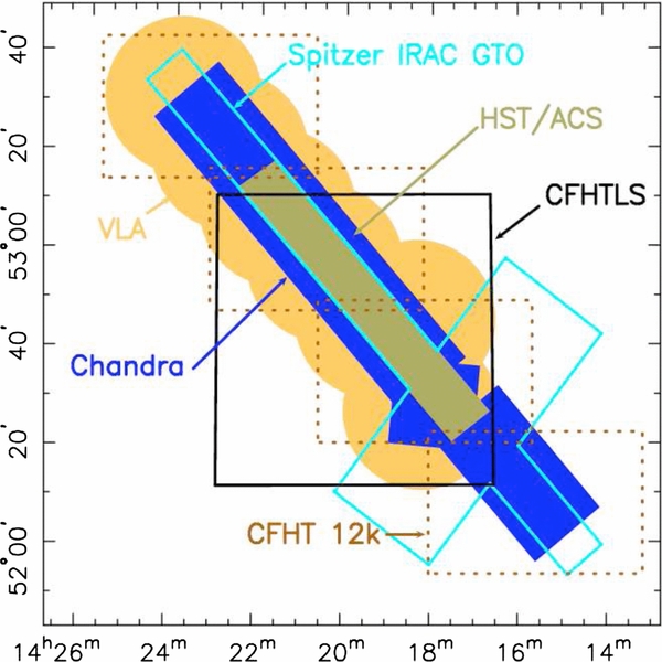
Figure 3. Initial data in the Extended Groth Strip (DEEP2 Field 1). Details of the individual data sets are given in Table 4. The CFHT 12K imaging provides the BRI pcat photometry used for DEEP2 target selection. The HST/ACS mosaic is one of the largest two-color V+I mosaics on the sky. The Guaranteed Time Observation Spitzer/IRAC data and the Chandra 200 ks data are the deepest/widest of their kind, and the CFHT Legacy Survey provides valuable synoptic variability data. EGS has also been imaged deeply with the VLA at 20 cm and with the GMRT (not shown) at 50 cm.
Download figure:
Standard image High-resolution image
Figure 4. Later extensions to the data sets in the Extended Groth Strip. Details of the individual data sets are given in Table 4. The FIDEL Spitzer/MIPS, AEGIS-X Chandra/ACIS, and GALEX/FUV+NUV imaging are the deepest exposures of their size on the sky. The follow-on DEEP3 survey (M. C. Cooper et al. 2013, in preparation) has increased the number of DEEP2 spectra by 50% and tripled the weight of environmental data in the upper three fields of EGS. The Warm Spitzer Extragalactic Deep Survey (SEDS) has provided a total of 10 hr of integration time per pointing in IRAC Channels 1 and 2 (centered at 3.6 and 4.5 μm). The NEWFIRM survey provides JK photometry to ∼24 AB mag, while the NEWFIRM Intermediate Band Survey (PI: Pieter van Dokkum; cf. van Dokkum et al. 2009) can measure photo-z's to roughly KAB ∼ 23.4. In addition (not shown), EGS is a deep SCUBA-2 Legacy field and a deep field for the Herschel HERMES survey with the PACS and SPIRE instruments, and is one of five fields selected for the multi-cycle treasury CANDELS survey being conducted with the Hubble Space Telescope (Grogin et al. 2011; Koekemoer et al. 2011).
Download figure:
Standard image High-resolution imageTable 4. Existing and Planned Data in DEEP2 Field 1 (Extended Groth Strip)a
| Data | Wavelength | Depthb | Areac | Contact |
|---|---|---|---|---|
| Keck DEIMOS (DEEP2) | 6500–9100 Å | R = 24.1 | 16' × 125' | M. Cooper |
| z = 0–1.4 | ||||
| Keck DEIMOS (DEEP3)d | 4800–9600 Å | R = 25.5 | 16' × 60' | M. Cooper |
| z = 0–1.4 | ||||
| MMT Hectospec | 4500–9000 Å | R = 22.5 | 17' × 120' | C. Willmer, A. Coil |
| GTC-EMIR GOYA | 1–2.5 μ | K = 24.5 | ∼0.3 deg2 | R. Guzmán |
| Chandra ACIS | 1–10 keV | 200 ks | 17' × 120' | P. Nandra |
| Chandra ACIS (AEGIS-X) | 1–10 keV | 800 ks | 17' × 40' | P. Nandra |
| XMM EPIC | 0.1–15 keV | 70–82 ks | 30' diam | ⋅⋅⋅ |
| GALEX UDeep imaging | FUV, NUV | 154, 270 ks | 125 diam |
S. Salim |
| GALEX grism | FUV, NUV | 291, 291 ks | 125 diam |
C. Martin |
| Hubble ACS | F606W, F814W | 28.7, 28.1 | 10' × 67' | A. Koekemoer, J. Lotz |
| Hubble ACS (CANDELS) | F606W, F814W | 28.9, 28.8 | 7' × 26' | A. Koekemoer |
| Hubble NICMOS | JH | 25.0, 24.8 | 0.013 deg2 e | S. Kassin |
| Hubble WFC3 (CANDELS) | F125W, F160W | 27.2, 27.3 | 7' × 26' | A. Koekemoer |
| CFHT 8K × 12K (pcat) | BRI | 24.5, 24.5, 23.5f | 4 × 28' × 42' | J. Newman, A. Coil |
| CFHT Megacam (CFHTLS)g | ugriz | ugri ∼ 27, z ∼ 25.5 | 1 deg2 | S. Gwyn |
| MMT Megacam | u'g'i'z' | 26.2, 27.2, 26.0, 26.0 | 1 deg2 | M. Ashby |
| LBT | UY | ∼25, 23.9 | 17' × 110' | B. Weiner |
| Subaru | R | 27.0 | 1 deg2 | M. Ashby |
| KPNO 4 m NDWFSh | BWRI | 27.1, 26.2, 25.8 | 1.4 deg2 | A. Dey |
| Palomar 5 m (POWIR)i | JKs | 23.9, 21.7–22.5 | 0.2, 0.7 deg2 | K. Bundy |
| CFHT WIRCAM | YJHK | ∼25 | 20' × 20' | R. Pello |
| CFHT WIRCAM (WIRDS)j | JHK | 24.8, 24.6, 24.5 | 3 × 20' × 20' | C. Willott |
| Subaru | K | 24.5 | 7' × 40' | T. Yamada |
| KPNO 4 m NEWFIRM | JK | 24.4, 23.9 | 1.4 deg2 | M. Dickinson |
| KPNO 4 m NEWFIRM (NMBS)k | JH(med.)j | K = 23.4 | 28' × 28' | P. van Dokkum |
| Spitzer IRAC GTO | 3.6, 4.5, 5.8, 8.0 | 0.9, 0.9, 6.3, 5.8 μJy | 10' × 120' | P. Barmby |
| Spitzer IRAC GTO (broader "handle") | 3.6, 4.5, 5.8, 8.0 | 1.0, 1.5, 9.3, 12.0 μJy | 60' × 25' | J. Huang |
| Spitzer IRAC (SEDS)l | 3.6, 4.5 | 25.7, 25.7 μJy | 12' × 75' | G. Fazio |
| AKARIm | 15 μ | 115–150 μJy | 10' × 70' | M. Im |
| Spitzer MIPS GTO | 24, 70 μ | 77 μJy, 10.3 mJy | 10' × 120' | J. Huang, R. Hickox |
| Spitzer MIPS FIDELn | 24, 70, 160 μ | 30 μJy, 3 mJy, 20 mJy | 10' × 90' | M. Dickinson |
| Herschel PACS (HERMES)o | 110, 170 μ | 5.2, 7.4 mJy | 10' × 67' | D. Lutz |
| Herschel SPIRE (HERMES)o | 250, 350, 450 μ | 11.1, 15.2, 12.9 mJy | 10' × 67' | S. Oliver |
| Scuba2 Legacy Deep | 850 μ | 3.5 mJy | 1 deg2 | R. Ivison |
| VLA | 6 cm | 0.6 mJyp | 30' × 80' | S. Willner |
| VLA | 20 cm | 100 μJy | 30' × 80' | R. Ivison |
| GMRT | 50 cm | 75 mJy | 10' × 90' | A. Biggs |
Notes. aPlanned or in progress are in italics. For a general overview, see http://aegis.ucolick.org/astronomers.html. bAll magnitudes are AB mags. Limiting magnitudes are 5σ unless otherwise stated; where none are available we list total integration time instead. cAreas are approximate. dDEEP3 has acquired ∼8000 new spectra and doubled the redshift sampling density in the Hubble ACS mosaic region. eNICMOS: 63 pointings. fCFHT pcat: 8σ. gCFHTLS: CFHT Legacy Survey (http://www.cfht.hawaii.edu/Science/CFHTLS). hNDWFS: NOAO Wide-Deep Field survey; EGS is an extension of the main NDWFS. iPOWIR: Palomar Observatory Wide Infrared Survey (Conselice et al. 2008). jWIRDS: WIRCAM Infrared Deep Survey (http://terapix.iap.fr/rubrique.php?id_rubrique=256). kNMBS: Newfirm Medium Band Survey; five medium-band filters from J through H (van Dokkum et al. 2009). lSEDS: Spitzer Extragalactic Deep Survey (G. Fazio 2010, private communication). mAKARI: 50% of the field is at the two quoted depths (5σ; M. Im 2010, private communication). nFIDEL: Far-Infrared Deep Extragalactic Legacy Survey (http://irsa.ipac.caltech.edu/DATA/SPITZER/FIDEL). oHERMES: Herschel Multi-Tiered Extragalactic Survey (http://astronomy.sussex.ac.uk/~sjo/Hermes). pVLA, 6 cm: 10σ (S. Willner 2007, private communication).
Download table as: ASCIITypeset image
To exploit the great richness of data in EGS, a broader research collaboration has been formed called AEGIS. This collaboration is combining efforts from more than a dozen teams who have obtained data in this field ranging from X-ray to radio wavelengths. More information on AEGIS may be found at the AEGIS Web site (http://aegis.ucolick.org) and in the 2007 May 1 special issue of the Astrophysical Journal Letters.
With Field 1 designated to be the EGS, Fields 2–4 were selected by finding regions free of bright stars, with low reddenings based on the IRAS dust map (Schlegel et al. 1998), spaced roughly 4 hr apart in R.A., and weighted toward higher R.A. where Keck weather is better. Their distribution also avoids the prime Galactic observing season and balances the number of nights required in each semester in order to ease telescope scheduling. The chosen fields all have declinations such that they are observable for more than 6 hr with an airmass less than 1.5, to ensure that differential refraction across a slitmask is below 02 (DEIMOS does not have an atmospheric dispersion compensator). Fields 3 and 4 are also in the multiply observed Equatorial Strip (Stripe 82) of the SDSS (York et al. 2000; Adelman-McCarthy et al. 2007; Ivezic et al. 2007) and are visible from both northern and southern hemispheres. The recently released deep SDSS photometry in this stripe should yield useful photometric redshifts down to DEEP2-like depths. A summary of complementary data available in these fields is given in Table 5.
Table 5. Existing Data in DEEP2 Fields 2–4
| Data | Wavelength | Deptha | Areab | Contact |
|---|---|---|---|---|
| Field 2 (16:52, 34:55) | ||||
| Keck DEIMOS/DEEP2 | 6500–9100 Å | R = 24.1 | 28' × 84' | M. Cooper |
| z = 0.75–1.4 | ||||
| Chandra ACISc | 1–10 keV | 9 ks | 30' × 100' | S. Murray |
| CFHT Megacam | i, z | 24.6, 23.2 | 1 deg2 | L. Lin |
| Palomar/KPNO 4 m (POWIR)d | JK | 22.4, 21.5 (variable) | 0.2 deg2 | K. Bundy |
| Spitzer IRACe | 3.6, 4.5, 5.8, 8.0 | 1.9, 2.9, 17, 21 | 45' × 100' | J. Huang |
| Spitzer MIPSf | 24, 70, 160 μ | 0.227, 40, 200 mJy | 0.7 deg2 | B. Weiner |
| Field 3 (23:30, 00:00) | ||||
| Keck, DEIMOS/DEEP2 | 6500–9100 Å | R = 24.1 | 28' × 126' | M. Cooper |
| z = 0.75–1.4 | ||||
| Chandra ACISc | 1–10 keV | 9 ks | 30' × 100' | S. Murray |
| CFHT Megacam | i, z | 24.6, 23.7 | 2 deg2 | L. Lin |
| SDSS Equatorial Stripe 82 | ugriz | ∼24 AB | All | ⋅⋅⋅ |
| Palomar/KPNO 4m (POWIR)d | JK | 22.4, 21.5 (variable) | 0.3 deg2 | K. Bundy |
| Field 4 (02:30, 00:00) | ||||
| Keck, DEIMOS/DEEP2 | 6500–9100 Å | R = 24.1 | 28' × 90' | M. Cooper |
| z = 0.75–1.4 | ||||
| Chandra ACISc | 1–10 keV | 7 ks | 30' × 100' | S. Murray |
| CFHT Megacam | i, z | 24.5, 23.7 | 2 deg2 | L. Lin |
| SDSS Equatorial Stripe 82 | ugriz | ∼24 AB | All | ⋅⋅⋅ |
| Palomar/KPNO 4 m (POWIR)d | JK | 22.4, 21.5 (variable) | ∼0.25 deg2 | K. Bundy |
| CFHT WIRCAM | J | 24.0 AB | 0.45 deg2 | L. Lin |
| Spitzer IRACg | 3.6, 4.5, 5.8, 8.0 | 4, 6, 25, 25 μJy | 0.95 deg2 | R. Hickox |
Notes. aAll magnitudes are AB mags. Limiting magnitudes are 5σ unless otherwise stated (where none are available we list total integration time instead). bAreas are approximate. cChandra ACIS program 9900045 (Goulding et al. 2012). dPOWIR = Palomar Observatory Wide Infrared Survey (Conselice et al. 2008). eSpitzer program 40689. fSpitzer program 40455. gSpitzer program 50660 (Jones et al. 2008).
Download table as: ASCIITypeset image
The original design of the DEEP2 survey consisted of 480 slitmasks. The expected number of 135 slitlets per mask would then target ∼65,000 galaxies, of which 52,000 were expected to yield secure redshifts assuming an 80% success rate. One can therefore crudely think of DEEP2 as having roughly twice the number of objects and three times the volume of the Las Campanas Redshift survey (Shectman et al. 1996), but at z ∼ 1 rather than at z ∼ 0.1. The design volume of 9 × 10⁶ h−3 Mpc3 would be expected to contain only a handful of rich clusters but is large enough to count both galaxies and groups of galaxies to good accuracy. At 1 hr per mask and eight masks per night, such a survey would take 60 clear nights of Keck time. Ninety nights were allocated via a Keck Large Multi-Year Approved Project proposal with Marc Davis as PI, which left a cushion of 50% for bad weather and equipment malfunction.
The above plan was followed closely, but the yield of reliable redshifts per galaxy targeted was only 71%, not 80%, owing to the fact that more galaxies than expected were beyond the effective redshift limit of z ∼ 1.4 (Section 11). Weather also did not fully cooperate, with the result that only 411 out of the 480 original slitmasks were observed, yielding a total of ∼53,000 spectra. The final area and numbers of slitmasks and targets observed in each field are given in Table 3, and sky maps of the regions covered are shown in Figures 1 and 2. The final survey observed 86% of the proposed number of slitmasks and 88% of the proposed number of galaxies.
5. DEEP2 IN COMPARISON TO OTHER z ∼ 1 SURVEYS
In this section and Table 6, we compare the properties of DEEP2 (considering both Fields 2–4 and EGS separately) to other large z ∼ 1 surveys in a variety of ways. The other projects considered include the TKRS in GOODS-North Wirth et al. 2004), the VVDS-deep survey in CDFS and in one other field (Le Fevre et al. 2005), the VVDS-wide survey in four fields (Garilli et al. 2008), zCOSMOS-bright in the COSMOS field (Lilly et al. 2007), and PRIMUS, which covers seven fields including several of the above (Coil et al. 2011).32 The first five are conventional spectroscopic surveys, but PRIMUS is a low-resolution prism survey yielding less precise redshifts but targeting many more galaxies. DEEP2 and TKRS have released all data, but the properties of the others have been deduced from stated plans and/or the available published data. Details of the data and sources used for these comparisons are given in the footnotes to Table 6.
Table 6. DEEP2 Compared to Other z ∼ 1 Surveys
| DEEP2 | DEEP2- | TKRSa | VVDS- | VVDS- | zCOSMOS- | PRIMUSe | |
|---|---|---|---|---|---|---|---|
| EGS | deepb | widec | brightd | ||||
| Fld name(s) | Fields 2–4 | Field 1 | GOODS-N | F02, CDFS | F02, 10, 14, 22 | COSMOS | 10 fields |
| Mag limf | 24.1 (R) | 24.1 (R) | 24.4 (R) | 24.0 (I) | 22.5 (I) | 22.5 (I) | 23 (I) |
| Spectral res, R | 5900 | 5900 | 2000 | 230 | 230 | 600 | 7–100 |
| Nom targsg | 45000 | 17775 | 2018 | 35000 | ∼100 K | 20000 | 270000 |
| Compl targsh | 35214 | 17775 | 1987 | 10949 | 31196 | ∼20000 | 270300 |
| Reliab z'si | 24785 | 12617 | 1536 | 4506 | 8961 | ∼11000 | 79419e |
| z err, km s−1 | 30 | 30 | ≲100 | 275 | 275 | 55 | 1800–3300 |
| Nom areaj | 2.80 | 0.60 | 0.046 | 2.0 | 16.0 | 1.7 | 10.0 |
| Compl areak | 2.18 | 0.60 | 0.046 | 0.61 | 6.1 | ⋅⋅⋅ | 9.1 |
| z's deg−2l | 11400 | 21000 | 21300 | 9400 | 2300 | 6600 | 8700 |
| zeffic1m | 0.711 | 0.717 | 0.725 | 0.399 | 0.280 | 0.565 | 0.45 |
| zeffic2n | 0.734 | 0.725 | 0.762 | 0.432 | 0.418 | 0.592 | 0.48e |
| Environ merito | 503 | ⋅⋅⋅ | 5.1 | 33.3 | 13.2 | 115 | ⋅⋅⋅ |
Notes. aWirth et al. (2004). bLe Fevre et al. (2005). cGarilli et al. (2008). dLilly et al. (2007, 2009). eA. Coil (2012, private communication). fMagnitude limit in AB mags. gNumber of target slitlets in survey as originally planned. hNumber of target slitlets completed to date. Includes stars but not serendips or (for DEEP2) objects without usable spectra (Q = −2). Roughly 1.1% of DEEP2 targets have Q = −2. iReliable galaxy redshifts to date with probability of correctness being ⩾95%, stars not included. For all surveys but PRIMUS, this means quality codes 3 and 4 or equivalent. VVDS-wide number includes bright galaxies that are also part of VVDS-deep. jTotal field area as originally planned, in square degrees. kTotal field area covered to date (single-pass only in parts of VVDS-deep and VVDS-wide). lReliable galaxy redshifts per deg2. Includes only galaxies with quality codes 3 and 4 (no serendips or stars) and attempts to be representative for non-uniformly covered surveys (VVDS-wide and VVDS-deep). DEEP2 numbers use galaxies in this paper and actual field areas minus regions lost to stars, CCD gaps, and incomplete mask coverage. TKRS is similar. VVDS-deep estimate uses existing redshifts in Field F02 with an assumed field size of 0.41 deg2; VVDS-wide estimate uses numbers of published galaxies in F02, F10, F14, and F22, which have mostly single pass; does not include the smaller area in F02, which is mostly double-pass. zCOSMOS-bright estimate uses the target density and star rate from Lilly et al. (2007) together with the reliable z-success rate measured from the zCOSMOS DR2 sample (Lilly et al. 2009) to predict a final density for Q3+Q4 galaxies of 10,400 galaxies per deg2. mOverall redshift efficiency, defined as the fraction of all targeted slitlets that yield reliable galaxy and/or QSO redshifts (⩾95%). Efficiency for VVDS-deep is calculated from the released set of 8981 redshifts, of which 35% have I < 22.5 and may also be in the VVDS-wide sample. nGalaxy redshift efficiency, defined as the fraction of targeted galaxies and/or QSOs that yield reliable redshifts (⩾95%). Total failures are allocated among stars and galaxies proportional to their numbers among the objects with successful redshifts; if all failures are in fact galaxies, the redshift efficiency would be lower than listed here. oFigure of merit indicating a survey's weight for environmental and clustering measures, given by N2/A, where N is the number of reliable redshifts (in thousands) and A is field area in degrees. Values used are the existing numbers for all surveys except zCOSMOS-bright, for which the design numbers are used. Combined numbers for DEEP2 and EGS are used. No entry is given for PRIMUS since its redshifts are not accurate enough to localize individual objects within the web of large-scale structure (which requires redshift errors significantly smaller than the correlation length, ≲ 500 km s−1; cf. Cooper et al. 2005). However, PRIMUS should provide accurate measurements of larger-scale overdensity around individual objects and can provide information on the relationship between galaxies and dark matter on smaller scales via projected cross-correlation functions.
Download table as: ASCIITypeset image
Given the significant redshift failure rate in all distant galaxy surveys, it is important to have a consistent definition of "redshift success." "Reliable," "secure," or "robust" redshifts are defined in this paper to be those with ⩾95% probability of being correct based on the identification of multiple features, according to their authors (for all surveys described, this means quality codes 3 and 4 (or equivalent, e.g., including codes 13, 14, 23, and 24 for VVDS), but not 1 or 2). In comparing surveys we use the sizes of the presently published data sets for all surveys except zCOSMOS, for which we use the design values.
We now proceed to compare the power of the various z ∼ 1 surveys using a variety of metrics. Numerical results are summarized in Table 6.
- 1.Redshift efficiency. A useful concept is "redshift efficiency," for which we offer two definitions. The first is the overall redshift efficiency, zeffic1, which is defined as the fraction of all slitlets (including stars) that eventually yield reliable galaxy (or QSO) redshifts. Values of zeffic1 are shown for the various surveys in Table 6. Apart from the two VVDS surveys, there is considerable degree of homogeneity in this quantity, with efficiencies hovering between 56% and 72%. With this definition, the efficiencies of VVDS-deep and VVDS-wide are only 28%–40%, partly because these surveys do not exclude stars, which hence take up a larger fraction of the slitlets than in other surveys, but mostly because of our high standard for redshift reliability, ⩾95% repeatability, which excludes many VVDS redshifts.The second definition of efficiency is the galaxy-only efficiency, zeffic2, which is defined as the fraction of galaxy-only slitlets that yield reliable galaxy redshifts.33 The percentages rise by 3%–4%, to 59%–76%, for the non-VVDS surveys and are now 42%–43% for the two VVDS surveys. The efficiency of VVDS-wide rises the most due to the high fraction of stars among its targets.
- 2.Volume sampled versus number of objects. Figure 5 compares the number of reliable redshifts versus volume sampled for both high- and low-redshift surveys. The volume used is computed from the areas in Table 6, bounded by the redshifts corresponding to the 2.5 percentile and 97.5 percentile point within a given survey (or by z = 0.2 and z = 1.2, the redshift range the team uses for science, in the case of PRIMUS). For surveys other than DEEP2 and TKRS (where the actual percentiles are used), these redshift limits are computed from analytic redshift distributions of the form
 , using fits to z0 as a function of limiting magnitude determined as described in Coil et al. (2004b), but using the full DEEP2 data set for calibration. This results in values of z0 of 0.26 for DEEP2 and TKRS, 0.224 for VVDS-wide and zCOSMOS-bright, and 0.283 for VVDS-deep. Among the contemporaneous distant spectroscopic surveys (i.e., excluding PRIMUS), DEEP2 has the best combination of total number and volume sampled, with 2.5 times as many redshifts as the next competitor, zCOSMOS-bright, and roughly twice its effective volume. PRIMUS surpasses DEEP2 and all other high redshift surveys in this space, targeting a larger number of galaxies over a larger volume (but with lower spectral resolution).
 - 3.Number density. Figure 6 uses the same data used to produce Figure 5 to compute cosmology-independent sample densities, expressed as the number of galaxies with secure redshifts per square degree per unit redshift interval; we also include the corresponding curve for the SDSS (for which we take based upon empirical fits to the data set) for comparison. Figure 7 converts this to the co-moving number density of objects, assuming our standard cosmology. The diamonds mark the median redshifts of the various surveys. The sample density is important since the statistical weight of a survey for environmental and small-scale clustering measurements increases as the square of this density if sky area is held constant (see below). Figure 7 shows that DEEP2/EGS is ∼4 times denser than zCOSMOS-bright and VVDS-deep in the redshift range z = 0.6–1.0 and ∼20 times denser than VVDS-wide. Both the higher secure-redshift rate and denser targeting of DEEP2 contribute to this difference. We omit PRIMUS from these figures and the environment figure of merit calculation (below) as the ability to determine local environment for individual objects in the PRIMUS sample is limited by redshift errors (σz/(1 + z) ≳ 0.005 ≳ 15 h−1 Mpc comoving) rather than sample number density; its number density is intermediate between that of zCOSMOS-bright or VVDS-deep and that of DEEP2.
- 4.Statistical weight for environment measures. A useful figure of merit that describes a survey's total statistical weight for environmental purposes (i.e., determining the average overdensity of the regions in which a given galaxy population is found) scales as N2/A, where N is the number of reliable redshifts and A is the area covered (assuming matching redshift distributions).34 This metric is given for the various surveys in Table 6 ("Env. metric"). The combined environmental weight of DEEP2+EGS will be four times that of zCOSMOS-bright when that survey is fully completed, and is 14–35 times the weight of VVDS-deep and VVDS-wide in their present states.
- 5.Spectral information. Other measures of survey power include spectral resolution and the total number of independent spectral resolution elements sampled. With a spectral resolution that is 10 or 26 times higher than zCOSMOS-bright or VVDS, respectively, DEEP2 is the only large deep survey that can measure the internal kinematics of galaxies, satellite motions, and small group velocity dispersions. Each DEEP2/DEIMOS spectrum has ∼2000 independent spectral resolution elements, as opposed to ∼320 for zCOSMOS-bright, ∼120 for VVDS-wide and VVDS-deep, and ∼20 for PRIMUS. Multiplying by the number of design targets (excluding stars) gives the total number of spectral elements present in galaxy spectra. By this metric, DEEP2+EGS has 16 times more information than zCOSMOS-bright, 10 and 33 times more information than VVDS-wide and VVDS-deep, and 185 times more information than PRIMUS. These figures are generous, as we have here assumed design numbers for total survey size and that all spectra in all surveys are equally likely to yield reliable redshifts once stars are excluded.
- 6.Galaxy counts. A final metric of survey power is the accuracy of galaxy counts. Two sources of noise contribute: Poisson statistics in the number of galaxies counted, and sample (or "cosmic") variance, which is determined by the number of fields, their areas, and geometries. Using the publicly available QUICKCV code of Newman & Davis (2002), we find that the cosmic variance in the count of a population of galaxies with r0 = 4 h−1 Mpc (comoving) and γ = 1.8 at z = 0.75–0.95 will be 7.6% for DEEP2, as opposed to 30% for TKRS, 14% for the completed area of VVDS-deep, 6.6% for VVDS-wide, 12% for the full zCOSMOS-bright area, and 5.1% for PRIMUS (here we assume square field geometry and equal area per field for all surveys but DEEP2; this will underestimate variance for VVDS-wide, as most redshifts are concentrated in a single field in that case). As a result, the noise in DEEP2 galaxy counts (e.g., measurements of the abundance of any particular population) will be smaller than in other distant z ∼ 1 grating spectroscopic surveys (though not than in PRIMUS); the larger sample size yields smaller Poisson errors, while the relatively long, narrow field geometry of DEEP2 gives smaller cosmic variance than would nearly square fields of the same area (Newman & Davis 2002).


Figure 5. Number of redshifts vs. volume sampled for major spectroscopic redshift surveys out to z ∼ 1. For all surveys except zCOSMOS-bright, we use the number of redshifts and areas covered to date (as given in Table 6 for the distant surveys). For zCOSMOS-bright, which is still in progress, design data are used. Numbers in all cases use reliable redshifts only (those with probabilities of being correct ⩾95%). Volumes covered are computed from the field areas and magnitude limits of each survey as described in Section 4. The TKRS survey is omitted from this figure (although included in Table 6) due to the relatively small sample size and volume. PRIMUS has low-resolution spectra, and provides coarser redshift information for brighter samples than the other higher-z surveys shown. If it is set aside, DEEP2 leads among distant surveys in both volume surveyed and number of reliable redshifts.
Download figure:
Standard image High-resolution image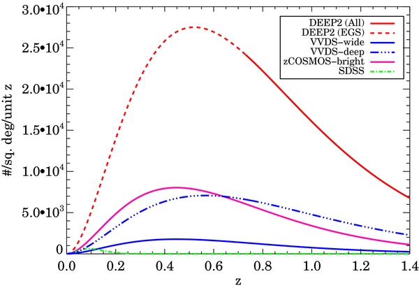
Figure 6. Sample number densities of various spectroscopic surveys, expressed as the number of galaxies per square degree per unit redshift interval (eliminating any dependence on cosmological assumptions). Curves are based on the stated magnitude limits, the number of reliable galaxy redshifts per square degree (⩾95%, see Table 6), and the redshift distribution model described in Section 4, applied to each survey. Note that the statistical weight of a survey for environmental and clustering purposes increases as the square of the co-moving number density if area and magnitude limit are held fixed. Because of its comparably high number density at z ≲ 1, DEEP2 is significantly better suited for environmental studies at intermediate redshifts than other deep surveys. The PRIMUS survey is not shown here, as in that sample spectral resolution, rather than sample number density, limits the ability to measure Mpc-scale environments for individual objects. Its number density at peak (z ∼ 0.4–0.6) is roughly 40% that of DEEP2, or approximately 50% larger than that of zCOSMOS-bright or VVDS-deep.
Download figure:
Standard image High-resolution image
Figure 7. Number densities of various spectroscopic surveys, expressed as number of galaxies per comoving Mpc−3 (assuming our standard ΛCDM cosmology). Curves are based on the same models and data used in Figure 6. Diamonds indicate the estimated median redshifts of each survey; an open symbol is for EGS for comparison to the other DEEP2 fields. Since the weight of a survey for environmental and clustering data scales as the square of the number density, the squares of the relative heights of the tick marks rank the surveys according to the strength of their clustering information per unit volume at their peak redshifts. DEEP2 and its EGS subset are the most densely sampled surveys shown, followed by SDSS, zCOSMOS-bright, VVDS-deep, and VVDS-wide. The number densities of all distant surveys considered decline roughly exponentially with redshift. As in Figure 6, the PRIMUS sample is not shown as its number density is not the limiting factor for small-scale environment measures; it is intermediate between the DEEP2 and zCOSMOS-bright surveys in this space.
Download figure:
Standard image High-resolution imageTo conclude, by all of these measures, DEEP2+EGS is more powerful than any contemporaneous high-resolution spectroscopic survey at z ∼ 1; in many cases, by a factor of 4–30×. This power enables a wide variety of unique scientific investigations. Of course, different figures of merit may be relevant for other types of studies than those considered here, but these areas of comparative advantage have led directly to much key DEEP2 science.
We have excluded PRIMUS in many of these comparisons; it has largely followed DEEP2 in time, and operates in a very different domain. Due to the very low resolution of its spectroscopy, redshift uncertainties are relatively large, ∼1800–3300 km s−1 (depending on redshift, due to the wavelength dependence of resolution in prism spectroscopy). This makes it infeasible to measure environment on ∼Mpc scales for individual objects (see Cooper et al. 2005), making our usual environmental figure of merit irrelevant. However, with nearly 80,000 redshifts over seven different fields, it has, by a significant factor, the lowest cosmic variance of any of these surveys and will be able to count rare objects and measure mass and luminosity functions for bright objects with unparalleled accuracy. It will also be effective at measuring clustering extending to relatively large scales; this allows measurement of the average overdensity of a population, an important measure of environment complementary to the measurement of overdensities for individual objects.
6. OBJECT SELECTION
6.1. Photometric Catalog and pgal Probabilities
The photometric catalogs used for selecting DEEP2 targets (the pcat catalogs, described in detail in Coil et al. 2004b) are derived from CFHT images taken with the 12K × 8K mosaic camera (Cuillandre et al. 2001) in the B, R, and I bands. These images were taken as part of a major weak-lensing survey by Nick Kaiser and Gerry Luppino, and we were very fortunate to piggyback on their efforts. The FOV of the camera is 28' × 42', as illustrated by the pointing boundaries in Figures 1 and 2.
The R-band images have the highest signal-to-noise ratio (S/N) and are used to define the object catalog, which is complete to RAB > 24.15 in all pointings. Objects were identified using the imcat software package written by N. Kaiser and described in Kaiser et al. (1995). This package was also used to calculate other image parameters used in object selection, such as object sizes and photometry. In Fields 2–4, the calibrated pcat catalogs for separate pointings are only utilized separately, and slitmasks in these fields were designed independently (though pointings overlap in Field 4, which means that one object can appear in two pcat's). In Field 1 (EGS), the pcat's were merged to make a single catalog for the whole area before the masks were designed (retaining the higher-quality photometry in overlap regions), so that each galaxy can appear only once. Each object is assigned an eight-digit object number; the first digit of the object number indicates the field the object was found in, the second digit indicates the CFHT pointing number, and the remaining digits provide a unique identifier, counting upward from zero. As an example, object 32001226 is the 1227th object in the pcat catalog for Field 3, pointing 2.
Objects with a high probability of being a star (i.e., a low probability of being a galaxy, pgal, as described in Coil et al. 2004b) were excluded when defining the pool of objects from which DEEP2 targets are selected. Figure 8 plots object radius rg versus apparent RAB magnitude, where rg is the 1σ radius in pixels of a circular Gaussian fitted to the CFHT photometry. The plot shown is for Field 3, pointing 2 (also referred to as pointing 32), which has seeing matching the overall median for the CFHT/DEEP2 data (084 FWHM); however, apparent object sizes are analyzed separately for each CFHT pointing. Stars are identifiable as the relatively tight, horizontal locus of points below and to the left of galaxies. Stellar radii increase at bright magnitudes due to saturation; the vertical line marks the point at which saturation becomes detectable in this particular pointing. Saturation sets in at RAB ∼ 16.7–18.0 depending upon pointing, establishing the bright magnitude limit for DEEP2 targets, RAB > 18.5.

Figure 8. Size–magnitude diagram resulting from pcat photometry in CFHT pointing 32, which has median seeing for the CFHT data set (084). Here rg is the rms radius in pixels of a circular Gaussian fit to an object's image (1 CFHT pixel = 0207). The stellar locus is visible as the narrow horizontal band below and to the left of galaxies. The left vertical red line is where stars begin to saturate, and the right vertical line is the magnitude limit of the DEEP2 survey, RAB = 24.1. The blue horizontal lines indicate the 95% size range for bright stellar sources in this pointing; it is determined individually for each CFHT pointing. The orange slanting line marks a line of constant surface brightness, 26.5 mag/□'', above which objects are excluded from DEEP2 targeting. Most excluded objects prove to be multiple objects incorrectly identified as single in the pcat photometry (see Section 12). Stars begin to blend with galaxies near R ∼ 22.5. A Bayesian probability for star–galaxy separation, 0 < pgal < 1, is calculated for all objects with size below the maximum of the stellar band by combining information on the magnitude and color distributions of stars and galaxies in DEEP2 (cf. Figure 9); objects with pgal < 0.2 are colored purple here. Section 6.1 provides more details on the algorithms used.
Download figure:
Standard image High-resolution imageInformation from the size–magnitude diagram in Figure 8 is used in conjunction with the B − R versus R − I color–color diagram to compute pgal; we summarize the classifications here, and refer the reader to Coil et al. (2004b) for details. First, objects with bad pixel or saturation flags set for their central pixel are assigned pgal = −2, and objects without a complete set of BRI magnitude measurements are given pgal = −1. Next, objects that have colors unlike any other stars or bright galaxies in the sample are given pgal = 2 (regardless of their size and magnitude, so long as pgal has not yet been set); this classification will not be overridden by that below. After those objects are excluded, the upper horizontal dashed line denotes the 95% upper radius range for stars (determined separately for each CFHT pointing), and all unclassified sources above this line are considered extended and assigned pgal = 3. However, stars have sizes indistinguishable from galaxies at dim magnitudes, particularly below RAB ∼ 23. In this regime, we can use the fact that stars tend to be brighter than and occupy a different locus in color–color space from compact galaxies to differentiate the two classes. The differences in colors are illustrated in Figure 9, which shows the BRI color–color diagrams for stars and extended galaxies in one DEEP2 pcat. For all objects having sizes consistent with the stars in a given pointing, the value of pgal indicates the net Bayesian probability that an object is a galaxy (as opposed to a star) based on both color information and brightness; it is therefore a value between 0 and 1. The red points in Figure 8 are the objects identified as likely stars, which we define as those having pgal < 0.2.

Figure 9. BRI color–color diagram for stars and galaxies. Gray points are candidate target galaxies in the Extended Groth Strip, i.e., they are objects in the pcat with 18.5 < RAB < 24.1 and pgal > 0.2. Stars, defined here as objects with pgal < 0.2, are indicated by the red points. Straight line segments show the boundary used for color pre-selection to screen out low-redshift galaxies in Fields 2–4; candidate objects at high redshift lie below and to the right of these lines. Specifically, the lines show the locus in color–color space where objects are given 10% weight for selection in Fields 2–4, the minimum possible for inclusion in the DEEP2 sample. The weight falls off from a maximum of 1 (a little below and to the right of this locus) as a 2D Gaussian having σ = 0.05 mag in both coordinates. This "pre-whitening" of the boundary is done to reduce the impact of any systematic color errors within a CFHT 12K pointing, which are of order 0.02–0.04 mag (Coil et al. 2004b). The division between objects treated as low- and high-redshift in EGS is similar to the lines shown (cf. Section 7.2). Stars are distinguished from galaxies by computing a Bayesian probability, pgal, based on the distributions of stars and compact galaxies in both magnitude and color–color space. Section 6.1 gives more details.
Download figure:
Standard image High-resolution imageTo summarize: negative pgal values indicate objects with problematic photometry. pgal = 3 indicates an extended source, all of which are included for target selection. Objects with peculiar colors have pgal = 2; these are also all taken as candidates (the vast majority have turned out to be objects with large photometric errors). Finally, values of pgal from 0 to 1 are used for compact objects with a size consistent with stars. More details are provided in Coil et al. (2004b). All objects with pgal > 0.2 are included as candidate targets for DEEP2, with selection weight proportional to pgal (to a maximum weight of 1). Further details on sample selection are given in Section 6.2, and possible biases are described in Section 8.
Note that the trajectory of stellar colors in Figure 9 is approximately described by two straight lines with a "knee" separating the two. Demanding that this knee be identical in all fields allows us to place all CFHT 12K pointings on a common color system, with an overall zero point determined via comparison to stars in the SDSS. From a variety of tests, we have found that pointing-to-pointing variations in the average photometric zero points are at the <0.01 mag level, while variations within pointings and absolute zero point uncertainties are ∼0.02–0.04 mag (Coil et al. 2004b).
6.2. Target Pool Selection Procedure
With pgal determined, a pool of potentially acceptable DEEP2 target galaxies can be defined. The final slitmasks are designed by selecting objects from this pool and placing them on slitlets. All galaxies selected as targets must fulfill three separate selection criteria that apply in all four DEEP2 fields.
First, the object must be classified as a potential galaxy by our probabilistic star–galaxy separation procedure. All extended objects and objects with peculiar colors are automatically included (pgal = 2 or 3). Objects whose sizes are consistent with stars are taken as eligible targets if they have pgal > 0.2, i.e., the probability of being a galaxy is greater than 20%. The distribution of pgal is extremely bimodal, with values piling up around zero or one (Coil et al. 2004b); as a result, varying the cut level between 0.2 and 0.8 makes very little difference to the sample.
The next cut is on apparent R-band magnitude: to be considered for DEEP2 targeting, an object must lie in the range 18.5 < RAB < 24.1.35 For science purposes, it would have been more ideal to use a redder band like I to set the survey magnitude limit, but the CFHT I photometry obtained was less uniform in depth, necessitating the adoption of R.36
Finally, the object must have a SB above a fixed limit (indicated by the slanting line in Figure 8). This SB requirement is defined by the equation:

where rg is the Gaussian profile radius for that object, here given in arcseconds. The minimum rg is set to 033, so that objects with 3rg < 1'' are presumed to have an effective 3σ radius of 1'' minimizing the effect of noise in measuring the sizes of compact objects on this cut. Visual inspection of the low-SB objects which are excluded by this cut indicates that nearly all are double or multiple sources in the BRI images that were incorrectly identified as single objects in the pcat due to blending. Their SBs are low because their radii are falsely inflated. Since the data for multiple objects are ambiguous, they are not good targets for DEEP2, and this cut properly excludes many of them.
The problematic deblending of these objects would affect counts of pairs within DEEP2 at separations corresponding to the distance between the two components. Almost all objects excluded by the SB cut have estimated Gaussian radii rg < 125, which generally roughly corresponds to the distance between the brighter and fainter component of the blend. We therefore can conclude that counts of pairs with separations ≲ 125 would be substantially negatively affected by the deblending algorithms used. This separation corresponds to a comoving separation of 14 h−1 kpc at z = 1 (or 7 h−1 kpc physical). For comparison, papers which have investigated DEEP2 pair counts exclude separations below 10 h−1 kpc physical from consideration, while DEEP2 clustering studies have excluded pairs with separations below 50 h−1 kpc comoving. We thus do not expect these deblending issues to have any significant effect on published science results, but advise users of the DEEP2 catalog to be cautious about conducting analyses which rely on counting pairs of objects with separations  . Further discussion of blended multiple objects may be found in Section 12.
6.3. Color Pre-selection in Fields 2–4
In Fields 2–4, the target pool is further refined to remove galaxies with redshifts likely to be below z ∼ 0.75. All but the bluest galaxies exhibit a significant break in their spectra at λ ∼ 4000 Å. This break causes a strong separation in color–color space between objects where the break falls in the B band or on the blue side of R, versus those where it occurs at redder wavelengths. We therefore use galaxies' B − R and R − I colors to identify the low-z interlopers. Since the bluest, flattest-spectrum objects exhibit minimal breaks (having colors near 0 at all redshifts), we always include those objects within our selection region in order to ensure that our sample is complete for galaxies at z > 0.75.
Figures 10–12 show color–color plots of galaxies in different redshift regimes in the EGS, where we obtained spectroscopy of galaxies at all redshifts (i.e., galaxies were not excluded based on this color cut). The lines show the nominal color boundary used to screen out low-redshift galaxies—essentially, only objects to the right and below this line are chosen in Fields 2–4, while objects of all colors are observed in EGS.

Figure 10. Assessment of the accuracy of the DEEP2 BRI color–color pre-selection for rejecting low-redshift (z < 0.7) galaxies. Gray points are the same set of DEEP2 candidate galaxies shown in Figure 9; red points are those EGS galaxies whose spectroscopic redshifts are below z = 0.7 (only secure, Q = 3 and Q = 4 redshifts are used). We here take advantage of the fact that low-redshift galaxies are not excluded from DEEP2 targeting in the Extended Groth Strip. The boundary is the 10%-weight locus repeated from Figure 9. Nearly all red points lie above the boundary, indicating that they would be successfully excluded from DEEP2 by the color–color pre-selection cut.
Download figure:
Standard image High-resolution image
Figure 11. Test of the accuracy of the DEEP2 BRI color–color pre-selection for galaxies near the transition redshift. This figure is similar to Figure 10, but colored points indicate EGS galaxies with spectroscopic redshifts in the range 0.70–0.75. Most of these lie below the boundary, indicating that they would be accepted by the color–color pre-selection cut despite their redshifts below 0.75. This is conservative, ensuring that objects with redshifts above z = 0.75 are not lost.
Download figure:
Standard image High-resolution image
Figure 12. Accuracy of color–color pre-selection for known high-redshift galaxies. This figure is similar to Figure 10, but colored points indicate EGS galaxies with spectroscopic redshifts above 0.75. Nearly all of these lie below the boundary, indicating that nearly all would be accepted by the color–color cut. The DEEP2 color selection produces a sample which is highly (approaching 100%) complete for high-redshift objects.
Download figure:
Standard image High-resolution imageThe boundary used is not perfectly sharp, but rather the weight given an object for selection falls off (from 1) as a 2D Gaussian with σ = 0.05 mag in both coordinates; we call the resulting weight the "color-weighting factor" for Fields 2–4 in the discussion below. This "pre-whitening" is done to reduce the impact of possible systematic color errors within a single CFHT 12K pointing, which are of order 0.02–0.04 mag (Coil et al. 2004b). The lines shown are not the nominal (i.e., sharp) boundary but rather depict the locus of points where the color-weighting factor equals 0.1 (i.e., 10%), the minimum for objects that will be selected for DEEP2 spectroscopy (for R − I < 0.2, the plotted lines are only approximately correct). Although this weight is used in target selection, selection probability is a slow function of the weight.37 The boundary in these figures corresponds to selection criteria for DEEP2 targets of
- 1.(B − R) < 0.5; and/or
- 2.(R − I) > 1.1; and/or
- 3.(B − R) < 2.45 × (R − I) − 0.2976.
The selection weight is 100% for objects with (B − R) < 0.389; (R − I) > 1.211; and/or (B − R) < 2.45 × (R − I) − 0.311.
Figure 13 demonstrates why we would expect such a color pre-selection to be effective. This figure shows the tracks of redshifted galaxy spectral energy distributions (SEDs) from Coleman et al. (1980, augmented by starburst galaxies from Kinney et al. 1996) in color–color space. Galaxies move across the color–color boundary rapidly as their Balmer and 4000 Å breaks move first through B − R and then through R − I near z = 0.7. The resulting valley in the colors can be used to sort galaxies into two groups below and above z ∼ 0.75.

Figure 13. Model color–color distributions for redshifted spectral energy distributions (SEDs) superimposed on DEEP2 targets. The SEDs used are based on spectroscopy of normal nearby galaxies from Coleman et al. (1980) and selected starburst galaxies from Kinney et al. (1996). Each SED executes a loop as the redshift increases as the Balmer/4000 Å break moves first through B − R and then through R − I at higher redshifts. Each model loop runs from z = 0 to z = 2.0 with diamonds shown at increments of 0.2; the line type switches from dashed to solid at z = 0.7. The lines are colored to improve visibility, with early-type spectra in red, later-types in purple, and starbursts in blue. The dashed lines are the boundaries used to pre-select target galaxies with z > 0.75 in Fields 2–4. Arrows indicate the impact of AV = 0.2 of extinction at a variety of redshifts. Dust reddening tends to move galaxies parallel to, rather than across, the DEEP2 color cut. These models are illustrative only—the final positions of the boundaries were tuned using EGS data, which contain galaxies at all redshifts.
Download figure:
Standard image High-resolution imageThe CWW (Coleman, Weedman, and Wu) models are illustrative only—the actual boundary was tuned using DEEP1 data and early redshifts in Field 1 (EGS), where all galaxies are eligible targets regardless of their color. Figure 14 shows the final redshift histograms of objects passing and failing the color cut in EGS. The vertical dashed line is the desired redshift cut at z = 0.75, and the 50%–50% crossover point is at z = 0.714. The crossover has been placed significantly below the target cut in order to enhance sample completeness at z > 0.75 (at the expense of somewhat decreased efficiency for targeting only high-z objects). Figure 15 shows the targeted fraction at all redshifts, which indicates the completeness of our color cut at a particular z. For the bin centered at z = 0.75, the pre-selection color cut correctly captures 91% of all objects and incorrectly rejects 9%. For bins above z = 0.8, these fractions are approximately constant at 97.5% and 2.5%, respectively. Figures 10 and 12 show that the loss of high-z galaxies and the creeping in of low-z galaxies are primarily due to blue objects in the lower-left corner of the color–color diagrams, whose colors tend to blur together at low and high redshift, as well as to objects with catastrophic photometric errors.

Figure 14. Redshift histograms for EGS galaxies with secure (Q = 3 or 4) redshifts that either pass or fail the pre-selection color cut. We correct here for the selection probability of each object, as otherwise the R-magnitude weighting scheme used in EGS would influence the redshift distributions (see Section 7). The 50%–50% crossover point has been deliberately placed at z ∼ 0.71 to insure high sample completeness above the nominal target redshift cut at z = 0.75 (vertical dashed line).
Download figure:
Standard image High-resolution image
Figure 15. Fraction of EGS galaxies passing the pre-selection color cut relative to the total number of galaxies with measured redshifts, as a function of z. Numbers are taken from Figure 14. This figure illustrates the high completeness of the color cut, which is 91% at z = 0.75 and averages 97.5% for 0.8 < z < 1.4.
Download figure:
Standard image High-resolution imageThe net effect of the color pre-selection in Fields 2–4 is to remove ∼55% of R < 24.1 objects from the target list—almost all unwanted foreground galaxies—with very minimal loss of the desired distant galaxies, and thus to increase the survey's efficiency for studying objects at the target redshift of z ∼ 1 by a factor of ∼2.2 at the cost of a ∼3% loss of desirable targets.
7. SLITMASK DESIGN
7.1. DEIMOS Detector and Slitmask Geometry
Having described the factors which determine whether an object is targeted by DEEP2, as well as the factors which contribute to their selection weight, we now turn to the methods used to design individual slitmasks from this target pool.
Our slitmask design algorithms intimately intertwined with the geometry of the DEIMOS detector array and slitmasks, which are illustrated in Figure 16. Related instrument parameters are given in Table 2. The telescope focal plane and slitmask geometry are shown as they are imaged onto the CCD detector array. For simplicity, we adopt the same coordinate system convention used for DEIMOS pipeline software outputs: "columns" run horizontally in the figure—i.e., parallel to the slitlet direction—while "rows" run vertically in the figure, parallel to the spectral direction. A typical extracted spectrum will therefore have 8192 columns but considerably fewer rows.38

Figure 16. Schematic of the DEIMOS focal plane, showing the geometry of the 2 × 4 CCD mosaic. The dispersion directions of the individual spectra run vertically. Superposed is a slitmask image as projected onto the detector in direct imaging mode. The TV guider camera stares directly at a fixed area of the focal plane. Light is reflected into the camera from the shiny slitmask (upper, light gray region) and more efficiently from a reflective mirror (lower, dark gray region). The geometry is precisely known, so that placing a given star at a predicted TV guider pixel at the proper spectrograph angle succeeds in placing the alignment stars for that mask within their respective 4'' × 4'' alignment boxes. Alignment proceeds by taking successive direct images through the mask followed by small corrections to the telescope R.A./decl. and spectrograph position angle. Flanking the main detector array are the flexure compensation CCDs. These are fed by ThAr emission spectra, which are piped into the slitmask focal plane by optical fibers (there are actually two fiber spectra at each end, but only one is shown). The ThAr spectra are so rich that at least one emission feature falls on the FCS CCDs at all grating tilts.
Download figure:
Standard image High-resolution imageThe CCD detector is composed of eight 2K × 4K MIT Lincoln CCDs with 15 μ pixels, for a total size of 8192 × 8192 pixels and total physical dimensions 126 mm × 126 mm. The CCD thickness is greater than normal (40 μ rather than 15 μ), which renders fringing negligible at wavelengths below 8000 Å and still yields low fringe amplitudes at longer wavelengths (e.g., only ±2% at 9000 Å). This thickness also boosts total system quantum efficiency at far-red wavelengths, e.g., to 16% at 9000 Å.39 The spacing between CCDs in the spectral direction is only seven pixels wide, while the gap between the long sides of the chips is roughly 1 mm, or  . A single spectrum in general falls on only two CCDs.
The slitmasks are flexible, flat aluminum sheets that are 23.6 cm wide, 75.7 cm long, and 0.50 mm thick. The total length of the mask on the sky is 167, while the maximum usable slit length (subtracting the CCD gaps) is 163. The masks are milled flat on a computer-controlled milling machine and spring-loaded onto a cylindrically curved mandrel in the spectrograph that approximates the spherically curved telescope focal surface. Eleven slitmasks can be held in a jukebox-like cassette at one time.
7.2. Mask Design Algorithm
The widest part of a DEIMOS slitmask projects to 52 across on the sky, but we place slitlets only within the inner 4' because the outline on one side is irregular. The wavelength range of the portion of the spectrum from a given slitlet which actually falls on the DEIMOS CCDs will vary according to slitlet placement. To maximize the wavelength range that is common to all objects (given anamorphic shifts in central wavelength with position on the sky), we select targets for spectroscopy only within a strip which is curved slightly "backward" on the sky, with edges corresponding to lines of constant wavelength on the detector.
To ensure good sky subtraction, we require that slitlets generally be at least ∼3'' long, implemented by requiring that successive targets be at least 3'' apart in the long direction of a DEIMOS slitmask (i.e., along a "row"). Objects are not placed within 03 of the end of a slitlet in order to ensure uniform slit width along each object, enabling accurate sky subtraction. We also require 06 of dead space in the slitmask's long direction between slitlet ends to limit cross-contamination between light from adjacent spectra (this is part of, rather than adding to, the minimum spacing between objects). The average slitlet length resulting from this procedure is 7''.
In Fields 2–4, the pattern of slitmasks on the sky is chevron-shaped, as shown in Figure 1. The two arms of the chevron are observed either east or west of the meridian to better align the slitlets with the atmospheric dispersion direction. Masks are designed separately for each of these two sets of masks; where they overlap at the point of the "V," some objects are observed multiple times, allowing tests of the repeatability of DEEP2 measurements. The slanting pattern also keeps the masks within the boundaries of the 28' wide CFHT 12K pointings, despite the masks being >14' long. Mask centers are separated along the long direction of a DEEP2 field by 2' on average, which gives each object roughly two chances to be included on a slitmask. The actual step size is modulated by an adaptive tiling scheme (see below).
The algorithm to place objects on masks in Fields 2–4 assigns each object a weight W between 0 and 1 that is the product of four factors. The first factor, WSG, comes from the star–galaxy separation probability pgal; it is unity if pgal = 2 or 3 but equals pgal if pgal is in the range 0 to 1 (i.e., for small galaxies or stars); only objects with pgal > 0.2 are considered for targeting. The second factor, Wc, which we will refer to as the "color-weight" is a measure of each object's consistency with the DEEP2 color–color cut. As explained in Section 6.3, this factor runs between 0 and 1 and is the result of smoothing a sharp-edged step function in the color–color diagram by a 2D Gaussian of width σ = 0.05 mag in each coordinate. Only objects with color weight >0.1 are considered for targeting.
The third factor, WR, is a function only of R magnitude and is designed to reduce gradients in the distribution of objects in redshift and magnitude. In Fields 2–4, this weight is given by the smaller of the two numbers (0.75 × 10−0.4*(R − 24.1)) and 1, which yields a weight that rolls off smoothly from 1.0 to 0.75 in the last 0.31 mag, de-weighting the faintest galaxies moderately. The final factor, applied only for DEEP2 objects observed in 2003 or later, is designed to reduce the number of high-redshift galaxies beyond z = 1.4 that are targeted, as they often fail to yield redshifts in DEEP2 spectroscopy. The target selection weights for these "blue corner" objects (those with B − R < 0.5 and R − I < 0.45) are multiplied by a factor Wbc that rises linearly from 0.1 for objects with R − I ⩽ 0.045 to 1 for objects with R − I ⩾ 0.45. Hence, in Fields 2–4, W = WSG × Wc × WR × Wbc.
In the EGS, pgal is still used for weighting, but no color pre-selection or blue-corner deweighting are applied, eliminating the second and fourth weighting factors. However, ignoring color information entirely yields a sample which is dominated by faint foreground galaxies. Therefore, a somewhat different form is used for the R-magnitude-based weight (WR) in this field.
Specifically, for EGS we calculate this weight factor differently according to which of two possible different scenarios applies:
- 1.If R < 21.5 or the galaxy passes the color cut to be at high redshift,40 WR takes the same value as it would in Fields 2–4, falling from 1 at R ⩽ 23.8 to 0.75 at R = 24.1.
- 2.If R ⩾ 21.5 and the galaxy fails the color cut (i.e., it is both faint and at low redshift), the weight is the lesser of the numbers 0.1 × 10−0.4(R − 24.1) and 1. This yields a weight that rolls off smoothly from 1.0 at R = 21.6 to 0.1 at R = 24.1, thereby decreasing the sampling rate for faint low-z galaxies.
As a result, distant EGS galaxies are weighted very like those in Fields 2–4 (except for small differences in the color boundary), while rare, intrinsically-bright low-redshift galaxies are given extra priority in target selection. In EGS, W = WSG × WR; but unlike in Fields 2–4, WR here depends indirectly on BRI color. We will summarize the effects of the two weighting schemes on the resulting sample at the end of this section, after describing the actual mask design process.41
In Fields 2–4, objects are allocated among the slitmasks in a two-stage process.42 The first pass places slitlets only in a central strip that is 2' wide on average (though this width can vary due to adaptive tiling, q.v. below). This central, curved strip is favored in order to maximize the wavelength region common to all spectra (with our chosen grating, the wavelength shift across 2' is ∼200 Å).
Cosmic variance in the number of targets within a 16' × 2' region is high, so that some masks will have fewer slitlets than others if masks are evenly spaced. To minimize this variation, we iteratively adjust the positions (and correspondingly the widths of the central regions) of masks in Fields 2–4 such that the number of targets selected in the first pass is held roughly constant from mask to mask (see Figure 17, which reflects these variations). This "adaptive tiling" strategy helps to ensure that a uniform fraction of target galaxies is sampled over the survey region.

Figure 17. Blowup of mask designs in a portion of CFHT pointing 32, showing a region near the "V" of the chevron pattern where many masks overlap. Dotted lines show the prime inner ∼2' strip within each mask (actual widths vary due to the adaptive tiling algorithm). Target objects are indicated by black ellipses with size 3rg and axis ratio (1 − e2). Slitlets on a given mask have the same color. Alignment stars are indicated by the red asterisks.
Download figure:
Standard image High-resolution imageAt the beginning of the first pass, the list of targets is temporarily trimmed by generating a random number between 0 and 1 and retaining only objects for which this random number is less than their weight. Thus, low-W objects (e.g., likely stars and galaxies just outside the nominal color cut) are only rarely placed on slits in this first pass. The trimmed list is then searched for cases where we can place two of the selected objects (separated by less than 3'' in the long direction) on a single slitlet that has a position angle (P.A.) relative to the long axis of the mask of less than 30°. Slitlets are allocated first to all such cases, boosting our ability to study close pairs of galaxies.
A random priority uniformly distributed between 0 and 1, P1, is then generated for each of the remaining objects in the trimmed list. Slit allocation then begins at one end of the mask (along its long axis) and proceeds to the opposite limit. Each object that can be observed without precluding the observation of any other is selected for observation; in cases of conflicts, the object with greatest P1 is taken. A new object will be allocated a slitlet only if it is more than a minimum distance along the long axis of the mask away from any object already targeted. This minimum buffer distance is the greater of 3'' or (03 + twice the radius of the new object projected along the slit, rg, proj), where the latter is computed from the new object's Gaussian radius rg, axis ratio, and P.A. New objects that are large must therefore be farther from existing objects and will be allocated longer slitlets as a result.
This procedure (initial selection according to W followed by nearly random selection among the surviving targets) yields a sample where the probability of selection is almost perfectly proportional to an object's weight, making the best possible use of the central portion of each mask. In Fields 2–4, 77%–80% of slitlets are allocated in the first pass.
After the first pass through all masks is completed, the remaining galaxies that overlap a given mask (over the full 16' × 4' area) are given new weight values W2 according to their initial selection weights, with W2 = (W/1–0.55W). This new weight accounts for the fact that the probability a given object is selected in pass 1 is very close to 0.55W, so the probability it is not selected is 1–0.55W. A new random number uniformly distributed between 0 and 1, P2, is then generated for each object; all potential second-pass targets are then ranked in descending order of W2/P2, providing a priority to each one. If all objects in pass 2 were subject to conflicts (i.e., have to compete with other objects for slitlets), this priority would ensure that the final probability an object is selected after passes 1 and 2 is proportional to its initial weight, W. The probability an object is selected in pass 1 is obviously proportional to W. To be selected in pass 2, an object had to not be selected in pass 1 (with probability (1–0.55W)); by ranking in W2/P2, objects are selected in pass 2 with a probability that is proportional to W2 = (W/1–0.55W). Thus, the net probability of being selected in pass 2 must be proportional to (1–0.55W)(W/1–0.55W)∝W as well.
Objects are then allocated slitlets in descending order of their priority, subject to the requirement that they do not conflict with any slitlet that has already been added to the mask (e.g., as an alignment star, in pass 1, or as an object with higher priority in pass 2). In the end, any target that can be placed on the mask without causing a conflict is included; as a result, in the second pass, low-weight objects will frequently be selected if they are cost-free. This causes the final selection probability of an object not to be simply proportional to W; in Fields 2–4, the probability is instead closely approximated by pselection = 0.27976 + 0.44717W − 0.09137W2. Hence, an object with a weight of 0.1 will be selected for observation 32% of the time, while one with W = 1 will be selected 64% of the time. Since most eligible targets have a weight near 1, the overall selection rate is close to the latter value. The second pass proceeds from west to east, assigning targets to all the masks in a row (i.e., all the masks with similar P.A.) in order.
The set of targets selected in the EGS differs in two respects from those in Fields 2–4. First, as noted above, there is no pre-selection based on color, and the R-magnitude-based weighting factor employed is different in order to suppress the number of faint foreground galaxies. The tile pattern in EGS is also different owing to the narrower width of the region, 16' rather than 30'. Masks are divided into eight groups with 15 masks per group, with each group approximately square in size (see Figure 2). In each square, eight masks have their long dimensions perpendicular to the long axis of the strip, and seven masks have their long axes parallel to the strip; masks parallel to the strip (within a given pointing) are given larger mask numbers.
In order to maximize the number of galaxies having measured rotation curves, we first divide all extended, clearly elliptical objects (those with eccentricity  > 0.081 (corresponding to axis ratio b/a < 0.85) and size 3rg > 1 arcsec) into two sets, one consisting of objects with their major axis within 45° of the long axis of the strip and the other including the remainder. The two-pass maskmaking algorithm described previously is then run on the set of objects in the second category, combined with those which are too small or round to have a well-defined P.A., to assign objects to masks that have their long direction perpendicular to the strip. Then, any galaxies not yet assigned to a mask, as well as the extended objects with their long axis aligned along the strip, are used to design the masks which have their long dimension parallel to the strip, again using our standard slit assignment algorithm. The crossed orientations again permit observations both east and west of the meridian and enable an expanded set of rotation curve measurements. However, in EGS the step size between masks is only 1' to allow for the greater density of targets on the sky; unlike in the other fields, the step size is not varied adaptively.
In EGS, 74% of objects on slitmasks are selected in the first pass, which again places targets only in the central 2' width of a mask. The second pass is similar to the second pass in Fields 2–4; again, galaxies are selected over the full 4' active width. By limiting the first pass selection to a field of only 2', the spectral coverage of the dispersed light for the galaxies is made more uniform. In the EGS, the probability an object is selected for observation depends on the weight W (which here is the product of WSG and the magnitude-dependent weight WR) as pselection = 0.33398 + 0.42687W; so an object with W = 0.1 is selected 38% of the time, while 76% of objects with W = 1 are targeted.
Once all objects are chosen, the final step is to set the lengths of the slitlets. Since no account was taken of the sizes of previously selected objects when new ones were added, it may happen that two projected buffer distances, each of size 2rg, proj + 03, overlap for two neighboring objects. In this case, the available space is evenly allocated between the objects, regardless of which one is larger. Much more commonly, when the separation is larger than the two buffer distances, the available slit lengths are allocated in proportion to their values of rg, proj. In both cases, half the dead space of 06 between slitlets is subtracted from the extent of each slitlet in the direction of overlap.
Once slitlets have been placed on targets, the design of all DEEP2 masks are adjusted to include ∼8 sky-only slitlets placed in open spaces on the masks. Their positions along the long axis of the mask are chosen to fall in-between the objects with largest separations, while their positions along the short axis are chosen to lie in empty regions (i.e., positions with no significant deviation from the background flux level within a 1'' radius) in the CFHT 12K images. The sky slitlets are used to perform fallback, "non-local" sky subtraction, which proved useful in dealing with some rare instrumental anomalies and, occasionally, for very short slitlets. These sky slitlets are only 07 wide; to produce a non-local sky model, the spectrum from a sky slitlet is convolved with a kernel that varies with wavelength, which is determined by a fit to each individual slitlet's estimated sky spectrum. In practice, this method proved inferior to local sky subtraction using the object's own sky spectrum, even for short slitlets, and it has therefore seen only limited use. However, non-local-sky-subtracted versions of both 1D and 2D spectra are included in the pipeline-produced data files for completeness.
As a final step, in order to preserve rotation curve information, the long axis of each slitlet is oriented as closely as possible along the major axis of its galaxy (as measured from the CFHT photometry), provided the following conditions are met: (1) the major axis of the object is within ±60° of the long axis of the mask, (2) the galaxy has rg ⩾ 1'', (3) the slitlet has not already been tilted to observe another object, and (4) the galaxy is measurably ellipsoidal, with CFHT axis ratio less than 0.85. As slitlet tilts, θ, can be up to 30° away from the long axis of the mask but no more, the mismatch between slitlet and galaxy P.A. can be up to 30° (except in cases where slits were tilted to cover multiple objects or for objects without measurable P.A.). We note that P.A.s measured from high-resolution ACS images can differ considerably from those determined from ground-based images, as found by Wirth et al. (2004).
In the central portions of a slitmask, slitlets are still tilted by ±5° compared to the mask direction for objects which do not fulfill these requirements. These small tilts ensure better wavelength sampling of the night-sky spectrum, improving sky subtraction (optical distortions provide the necessary sampling for untilted slits at the ends of a mask, so those slitlets are designed with P.A. = 0 relative to the mask's long axis). The crosswise widths of tilted slitlets are reduced by cos(θ) in order to maintain a fixed projected slitwidth along the dispersion direction.
Figure 17 shows a blowup of a region covered by several slitmasks in Field 3, with the central first-pass regions, eligible targets, selected targets, and slitlets with their final lengths and orientations all plotted. The overlap of slitmasks at the "V" of the chevron pattern provides a sample of multiply observed objects for statistical and reliability assessment purposes; we make use of this information in Section 11.3.1, below.
In the end, 61% of eligible targets are assigned slitlets in Fields 2–4. More precisely, this is the fraction selected out of targets that have 18.5 < R < 24.1 and pgal > 0.2; pass the SB cut; and have probability >0.1 of meeting the color–color cut. Slitmasks in these fields contain ∼110–140 target slitlets (mean 121) that are typically 7'' long but span the range 3''–15+''.
In EGS, the average number of slitlets per mask is 148. In pointings 11–13 of EGS (the southern three-fourths of the field), R-band de-weighting of low-redshift galaxies boosts the relative number of high-z galaxies, with the result that, of those targets that would have been eligible for selection in Fields 2–4 (as described above), roughly 73% are selected in EGS.43 In contrast, due to the deweighting of faint objects that fail the color cut, only 53% of low-z galaxies are selected. Without this deweighting, only 55% of the galaxies in a Field 2–4 equivalent sample would have been selected, which would have made the sample sparser in number density at high redshifts than the other DEEP2 fields.
8. SELECTION EFFECTS IN THE FINAL TARGET SAMPLE
The final DEEP2 target sample suffers from a variety of known selection effects. These effects should in general be taken into account and/or corrected for when utilizing the DEEP2 data set. A variety of methods for doing so have been implemented in DEEP2 science papers; see Section 3 and Table 1 for examples.
- 1.Galaxy color bias due to the R magnitude limit. Selection according to a fixed apparent R-band magnitude limit causes the resulting sample to reach different depths (in terms of absolute magnitude) for galaxies of different intrinsic colors at the same redshift. At z ∼ 0.5, the R-band filter corresponds closely to restframe B, so objects are selected down to the same B-band absolute magnitude independent of color. Below that redshift, R-band selection favors redder galaxies, while above this, it favors bluer galaxies. The effect was first illustrated in Willmer et al. (2006) and is discussed in more detail in Section 15. Though fundamental, this bias is well understood and can readily be applied to mock catalogs and other statistical predictions. The same type of bias will inevitably affect any magnitude-limited sample which spans a range of redshifts, due to the broad span of intrinsic galaxy colors.
- 2.Loss of bright star-like objects. The use of pgal discriminates against point sources (i.e., objects with apparent size consistent with stars; cf. Figure 8), and thus potentially discriminates against bright Type I AGNs, i.e., QSOs. AGNs will be lost only if they are both point-like and lie on or near the stellar locus in the color–color diagram. As a result, Type I AGNs will be included in the DEEP2 sample at some redshifts, but excluded at others.
- 3.Misclassification of faint stars as galaxies. Although the differential number counts of objects classified as stars (pgal < 0.2) in the DEEP2 pcat's rise approximately linearly at bright magnitudes, they flatten out at RAB ∼ 22.5; it is likely not coincidental that this is where large numbers of galaxies begin to populate the stellar regime in Figure 8. It appears that the pgal values overestimate the probability that faint objects are galaxies rather than stars; we therefore tend to include more stars than expected within the DEEP2 target list. This is conservative from the standpoint of galaxy selection, as the contaminant objects are trivial to weed out once spectra are obtained.44 However, as a result of this misclassification, a list of photometric stars selected purely via their pgal values will be incomplete at the faint end and would be of limited use for stellar studies.
- 4.Loss of objects due to missing B or I photometry. The definition of pgal and the DEEP2 color pre-selection both depend on having measured B − R and R − I colors.45 Though the R-band photometry is complete to the RAB = 24.1 magnitude limit in all fields (Coil et al. 2004b), very red or blue objects may not be detectable in either the B or I imaging. However, in the three EGS pcat pointings with accurate B and I photometry (11–13), which contain 59,594 objects brighter than RAB = 24.1, only 153 galaxies are missing B. They tend to be faint and red and constitute only 4% of distant (red-sequence) galaxies with RAB > 23 and R − I > 1.0. Their loss is not significant. Similarly, 71 galaxies with RAB < 24.1 are not detected in I; they are predominantly very blue. We expect similar rates of loss in other DEEP2 pointings.
- 5.Loss of small, distant, faint red galaxies. Our Bayesian method for discriminating faint stars from galaxies depends on the contrast between stars and galaxies in a color–color plot (Figure 9), as well as on the fitting functions used for the magnitude distributions of each class. The blue stellar locus is quite narrow, so the loss of blue galaxies misclassified as stars is fractionally small. The situation changes where B − R > 1.5 and R − I > 0.6, where the surface density of stars becomes more comparable to that of galaxies. As shown by Figure 13, this region of the color–color plot is populated by intrinsically red galaxies beyond z ∼ 0.7. Loss of such galaxies was estimated by Willmer et al. (2006) using the higher-resolution HST ACS images in EGS and partial redshift data. We redo that calculation using final EGS redshifts and a larger database.Figure 18 plots the color–color diagram for EGS but restricts to objects in the ACS mosaic fainter than R = 23.0, where misclassification is most likely (cf. Figure 8). DEEP2 stellar candidates (pgal < 0.2) that are confirmed as stars in EGS ACS images are plotted in blue; those shown instead to be galaxies are red. The latter are missed by DEEP2 and are thus a concern. Galaxies are lost in a narrow band in B − R, which corresponds to certain combinations of intrinsic red-sequence color and redshift (cf. Figure 13).The central rectangle in Figure 18 delineates the region in which galaxies are lost. Setting true stars aside (the blue points) leaves a total of 99 galaxies in the rectangle, of which 27 were misclassified as stars by pgal (red points). However, only about half of all R > 23 red-sequence galaxies at z = 0.75–1.1 lie in the rectangle—the others lie in the rectangles above or below—and this fraction is found to be virtually constant at all redshifts above z = 0.75. Since galaxies outside the central rectangle are not lost, the net result is that ∼0.27 × 0.50 ∼0.13=13% of red-sequence galaxies in the dimmest magnitude bin are lost, and this loss is uniform beyond z = 0.75. This matches the estimate of Willmer et al. (2006). A loss of this size is not generally important for analyses of total counts along the red sequence but might be important (effects as large as 27%) for studies in individual restframe color bins within the red sequence that have apparent B − R near 2.25.
- 6.Loss of objects at small separations. Because spectra of galaxies on the same mask cannot be allowed to overlap, the number of slitlets that can be put down in a small area is limited for objects that would have similar positions on a mask (along its long axis); this affects the sampling rate in dense regions. This effect is illustrated in Figure 19, expanded from Gerke et al. (2005), which shows that the sampling rate in the very densest regions (in terms of nearest neighbor distance on the sky) is reduced by almost a factor of two from nominal, but that the fraction of sampled galaxies that yield reliable redshifts is unaffected. The upturn of the sampling rate at small separations is due to the placement of close pairs on a single slitlet.It should be noted that this effect is much weaker as a function of three-dimensional density: unlike in nearby galaxy surveys like SDSS, most conflicting objects (and most sets of nearest-neighbors on the sky) are actually at very different redshifts from each other (a consequence both of L* brightening with z and the comparatively small contrast in luminosity distance between z ∼ 0.7 and z ∼ 1.4). The effect is already substantially smaller in impact than fiber collisions in nearby-galaxy surveys, since in DEEP2 objects can conflict with each other along only one dimension, and even then only at scales not much larger than an individual galaxy (1'' spans ∼10 h−1 kpc comoving at z = 1, while the minimum separation between objects along the mask direction—i.e., the separation within which they conflict with each other—is 3'').Nonetheless, the diminished sampling rate in dense regions is a large enough effect that it needs to be taken into account for certain statistics. For example, Coil et al. (2001) investigated the impact of prototype DEEP2 target selection algorithms on the ξ(rp, π) diagram; they found that it introduces moderate distortion into the two-point redshift-space autocorrelation function at small projected separations, reducing the elongation of contours along the "finger of God" by about 20%. The data shown in Figure 19 can be used for modeling purposes. In all DEEP2 clustering analyses (e.g., Coil et al. 2006a, 2008) this effect is quantified and corrected using mock catalogs that have been passed through the DEEP2 target selection code.
- 7.Multiple galaxies masquerading as single galaxies. The final known bias in the DEEP2 target sample is due to the finite resolution of the CFHT BRI ground-based images, in which separate galaxies may appear blended. This blending can distort the magnitudes and colors of DEEP2 galaxies, and it can also elevate galaxies that would otherwise be too faint to meet the RAB = 24.1 magnitude limit above that threshold. Investigating these composite objects requires redshift information, and so this topic is deferred to Section 12 after DEEP2 spectroscopy, data processing, and redshift measurements have been discussed.

Figure 18. Color–color diagram for faint (R > 23) objects in the Extended Groth Strip with HST/ACS imaging. This is the domain where we expect confusion between stars and galaxies to be most likely, based on Figure 8. Objects classed as stars based on the CFHT 12K photometry (pgal < 0.2) are the colored points. Objects confirmed as stars in the ACS images are blue; those which proved to be galaxies are red. The red points are missed by DEEP2 and are thus a concern. The loss is worst (as a fraction of all objects) in the dashed rectangle, where high-redshift red sequence galaxies in the range z = 0.75–1.0 cross the stellar locus. The loss within that rectangle is 27%. However, roughly half of galaxies in the affected redshift and parameter regime lie in the upper and lower rectangles, which are not lost, giving a final estimated loss fraction of ∼13.5% (see Section 8).
Download figure:
Standard image High-resolution image
Figure 19. Rate of spectroscopic observations and redshift success as a function of local density of DEEP2 target galaxies on the sky, as measured by the third-nearest-neighbor angular distance, D3. Upper panel: dashed lines show the probability that a galaxy meeting the DEEP2 targeting criteria receives a slitlet. The heavy solid lines give the total probability that its redshift is reliably measured (Q ⩾ 3). The light solid lines repeat this with all galaxies in the blue corner excluded, as most of those do not yield reliable redshifts. The top axis shows the cumulative percentage of z ∼ 1 galaxies with D3 up to a given value. Vertical lines show the apparent sizes of dense cluster cores at two redshifts (co-moving). The sharp increase in targeted fractions at low D3 arises because close pairs may be placed on a single slitlet. The lower panel separately shows the redshift success rate once a galaxy is targeted. The probability of observation is reduced by almost a factor of two in regions of high density, but redshift success rate is unaffected.
Download figure:
Standard image High-resolution image9. SPECTROSCOPIC PROCEDURES
Instrument and exposure parameters for the DEEP2 survey are summarized in Table 2. Each mask is observed for at least three 20 minute exposures with the DEIMOS 1200 lines mm−1 gold-coated grating centered at 7800 Å. No dithering is performed between exposures because sky subtraction is natively almost photon-limited (see Section 10.2), and dithering would waste roughly half of the detector real estate.
The DEIMOS guider camera is rigidly mounted in the slitmask coordinate frame with known orientation and offset (Figure 16). Locating a guide star at a precomputed pixel location while the mask is at the proper P.A. therefore succeeds in placing all alignment stars within their 4'' square slitlets. In a direct image of the night sky through the mask, the locations of alignment stars and of all slitlets, including the alignment boxes, are visible (the latter are illuminated by the sky and hence much brighter than the interslit background).
We obtain the necessary direct alignment images efficiently by tilting the grating to zeroth order, rather than swapping the grating for a mirror; the images obtained are then analyzed using custom-designed software using a graphical interface. The pointing of the telescope and the P.A. of DEIMOS are then adjusted to center all alignment stars within their boxes, which in general centers all galaxies in their slitlets to within 01 (modulo astrometric errors). Slitmask alignment generally converges after two direct images and takes roughly five minutes. It is generally checked once using the same procedure after the first of the three spectroscopic exposures (see below).
The fraction of wavelengths common to all spectra is shown in Figure 20; 50% coverage limits are 6500 Å–9100 Å. The 10 slitwidth used for all targets yields OH skylines with an FWHM of ∼1.3 Å, which produces a spectral resolution R ≡ Δλ/λ = 5900 at 7800 Å. A custom data verification program called quicklook46 is run during observing. This program performs a coarse reduction of 10% of the slitlets on each exposure and computes the cumulative S/N for an R = 23.5 source obtained by combining all exposures so far. We continue obtaining exposures until a minimum S/N threshold is met, which enables productive observing even under clouds or poor seeing. The quicklook software also checks for missing lamps in arcs, the occasional slitmask buckling, FCS misalignments, guiding errors along the slit, and bad or degrading seeing (based on the FWHM of the alignment star spectra). Run on a Sun workstation from circa 2002, it is able to evaluate a single DEIMOS frame in roughly 10 minutes (compared to our 20 minute exposure time).

Figure 20. Fraction of DEEP2 spectra having coverage at a given wavelength. The dip around 7800 Å is due to the gap between blue and red chips in the DEIMOS detector; this gap falls at different wavelengths for different spectra due to variation in slitlet position along the wavelength direction.
Download figure:
Standard image High-resolution imageAll slitmasks are observed at airmass below 1.5. Under optimal conditions, eight masks can be observed per night, yielding 1000–1200 spectra.
10. REDUCED SPECTROSCOPIC DATA
10.1. The spec2d Data Reduction Pipeline
The DEIMOS spec2d pipeline (Cooper et al. 2012b) is an IDL-based code that is modeled on and borrows significant code from the SDSS spectral pipeline of David Schlegel and Scott Burles (Schlegel & Burles 2012). Most of it was written by Douglas Finkbeiner, Marc Davis, Jeffrey Newman, and Michael Cooper, with important contributions from Brian Gerke regarding non-local sky subtraction (see below). The pipeline operates in five separate stages, each of which produces its own output files. The code operates without supervision and usually does an excellent job of wavelength fitting, sky subtraction, and object fitting.47
The first step in data reduction is creation of a "planfile" (a plain-text file with extension.plan) which may be generated automatically after a night's observing and defines the locations of all files needed to reduce a given mask's data. The planfile may optionally control various parameters of the reduction such as the chips to be reduced, the arc line list to be used, etc. The planfile is used by a controlling IDL program, DOMASK, which calls separate routines which perform a series of reduction steps.
Step I. The first stage of data reduction is to produce calibSlit files (i.e., a set of FITS BINTABLE format files whose filename begins with "calibSlit") from the flatfield and arc frames taken through a given mask. This processing is controlled by the IDL procedure DEIMOS_MASK_CALIBRATE. Each of the eight DEIMOS CCDs is analyzed completely independently through all stages of the 2D reductions, allowing trivial parallelization; in general, every spectrum will span two of these eight CCDs, which we will generally refer to as "blue" and "red"; hence for each object's spectrum there are two separate calibSlit, spSlit, and slit files (q.v. below). The calibSlit files indicate where the slitlets fall on the CCD array for each mask and contain flatfield information and a 2D wavelength solution for each slitlet.
To produce the calibSlit files, first the multiple flats are read in, corrected for pixel-to-pixel response variations, and processed to reject cosmic-rays. To identify every slitlet, edges that are detected in the flats using an unsharp mask are compared to a table in the DEIMOS header data that describes where each slitlet should appear; a smooth polynomial is fitted to the edges of each curved spectrum to define its upper and lower limits. Each chip's combined flat frame is then mapped into rectangular arrays for each slitlet, which greatly simplifies further processing, by shifting its edges to be parallel, using interpolation (over the spatial direction) to accommodate subpixel shifts. Hence, we turn the entire flatfield image into a set of individual rectangular flatfields for each slitlet. Each slitlet's flatfield is first used to measure the "slit function," i.e., the relative throughput (maximum 1) of each slitlet as a function of position (i.e., row number) along it.48 After normalizing by the slit function and any large-scale variation in light intensity with wavelength and position along a given slitlet, the flats are smoothed on small scales to generate a 2D fringing-correction map with mean 1.
Step II. The next step, also controlled by DEIMOS_MASK_CALIBRATE, is to solve for the wavelength of each pixel in the 2D data array. First, the entire arc (or arcs, if multiple ones are available49) is read in and corrected for pixel-to-pixel response variations. Next, a single shift in the spatial direction between a given chip's arc data and the original flatfield, dx, is determined by finding the lag which maximizes the cross-correlation between the intensity summed over the central (in the wavelength direction) region of the arc frame with the light profile predicted from the slit edges found in Step I (only whole-pixel shifts are considered). Then, individual slitlet arc spectra are extracted and rectified in the spatial direction using the same algorithms applied for the flatfield, but using slit edges shifted from the flat by dx; the individual spectra are then corrected for the slit function and fringing using the results of Step I.
Starting with the DEIMOS optical model (produced by Drew Phillips), which gives a rough initial guess, we fit for the relationship between wavelength and pixel in a spectrum in multiple stages, obtaining a wavelength solution that is typically accurate at the 0.007 Å (∼0.02 pixel) rms level or better over the entire 2D spectrum; 0.003 Å rms is commonly achieved. The fits used are linear regressions for the coefficients of Legendre polynomials of up to fifth order (for wavelength as a function of pixel number along the central row of the slitlet) or second order (for specifying the local tilt of the constant-λ locus as function of central pixel number). The mean residual about the fit in each row of the slitlet is also stored and incorporated into the wavelength solution (i.e., we apply a row-by-row shift from the smooth polynomial-based solution, which can account for defects or dust along the slit which shift the mean wavelength of a row). The requirements that accurate OH-line subtraction places on sky subtraction are discussed in Section 10.2 and in the Appendix. We generally require errors below ∼0.01 Å rms for good sky subtraction; to be useful in attaining wavelength solutions, individual arclines must contain ∼10,000 photons in each row. The result of Steps I and II is a single calibSlit file containing all necessary calibration information per slitlet per chip (i.e., each spectrum is split into blue and red files).
Step III. The third stage of the reductions, controlled by the procedures DEIMOS_2DREDUCE and DEIMOS_SPSLIT, uses the calibSlit files produced in Steps I and II to flatfield and rectify the on-sky ("science") data for each slitlet. Response correction, slitlet extraction/rectification, and flatfielding are all done using the same procedures as for the arc files. All CCDs are again treated separately. An inverse-variance image is also produced based on the photon and read noise (with compensations for all multiplicative corrections applied), as well as maps of bad pixels (which will have zero inverse variance; this map provides flag information on why a given pixel is bad) and questionable ones (e.g., those which may be affected by imperfect vignetting corrections or cosmic rays, which will not have their inverse variance set to zero; again, this map provides flag information for each pixel).
The most important operation in this step is computing the proper sky background level (including bright OH lines) at every location in a 2D science spectrum as a function of both wavelength and position along the slitlet. First, a constant wavelength shift (relative to the arc wavelength solution) for each frame is determined using cross-correlation against a high-resolution night-sky spectrum. Then, a B-spline model for sky intensity as a function of wavelength is fitted to the sky regions of the slitlet (i.e., regions where, based on their location and size, both contamination from DEEP2 targets and slitlet edge effects are expected to be minimal). A key stratagem is tilting all slitlets by at least 5° with respect to the detector array so that each night sky line is substantially oversampled, making the B-spline fit more accurate; see Appendix A.4. The result of Step III is one spSlit file per slitlet per chip, which contains the reduced 2D spectra (with associated wavelength, inverse variance, and mask arrays) from each science frame for that slitlet and that frame's B-spline fit in alternating HDUs.
Step IV. The fourth stage, controlled by SPSLIT_COMBINE and SLITEXAM, combines the separate science exposures for each slitlet into one inverse-variance-weighted mean, sky-subtracted, cosmic ray-cleaned 2D spectrum (which we will generally refer to below as a "combined" or slit file). First, the B-spline model sky for each slitlet is subtracted from its flux. Next, the (generally) three 20 minute exposures are combined, weighting them according to the inverse variance maps from the previous stage. Cosmic ray rejection is also done at this time based on the time variability of a given pixel. The result of this process is one slit file for each slitlet for each chip, containing the processed, combined 2D spectrum, inverse variance, and wavelength solution, along with various diagnostic information (e.g., bad pixel masks). Each row of each spectrum has its own wavelength solution; a 2D map of wavelength as a function of position in an image may be obtained with the IDL function LAMBDA_EVAL.
Step V. In the fifth and final stage, 1D spectra are extracted from the combined 2D spectrum using the routine EXTRACT1D (controlled by the procedure DO_EXTRACT). Extraction is done using both "optimal" and boxcar (i.e., fixed-width sum) extraction techniques (see below), as usual processing the blue and red chips separately. As a first step in both approaches, each 2D spectrum is rectified in the wavelength direction by using whole-pixel shifts (as opposed to interpolation), making the wavelength scale in each row match the central row of the object.
The optimal extraction (or "horne" as it is labeled in the FITS headers) loosely follows the algorithm of Horne et al. (1986). However, due to the lower S/N of some DEEP2 data, instead of using the light profile evaluated at a single location along the slit to weight pixels, a Gaussian model is used for weighting. First, we measure the light profile along each slit by performing an inverse-variance weighted average of the flux along each row of the slit, excluding regions around bright night sky emission lines. Next, an overall offset between the positions of objects along each slit predicted from the mask design and their actual observed positions is determined by fitting a Gaussian to each peak in the individual slits' light profiles and comparing their locations to the prediction. We also determine the quantity that must be added to or subtracted from (in quadrature) the sizes of objects in the CFHT photometry (rg values) to match the observed widths of each Gaussian peak, allowing compensation of sizes for differences in seeing. The center of the extraction window is determined from either the peak of the spatial profile of the object along the slit or (in low-flux cases where the peak differs by at least 5 pixels from the prediction) using the predicted position with the just-determined shift in the spatial direction applied. The extraction center is determined independently on the red and the blue sides, ameliorating the small shifts between them expected due to differential refraction.
The weighting kernel P used for optimal extraction is then a Gaussian with peak at the center of the extraction window and σ derived from a Gaussian fit to the light profile in the 2D spectrum in high-S/N cases, or the expected seeing-corrected size as derived from the photometry in the event of low S/N. In our reductions the extracted flux f at a particular wavelength is

where fi is the flux, Pi is the model profile, and Si is the inverse variance at a particular row (at fixed wavelength). Including the inverse variance in the weight in this way yielded slightly improved results over using the Gaussian profile alone.
In the boxcar approach, bad pixels are masked (rather than interpolated over as in the optimal extraction) and the fraction of flux missed within these pixels is determined using the Gaussian model spatial profile along the slit determined for the optimal extraction. The flux from all pixels at a given wavelength is then summed, and that sum is divided by the fraction of flux which should have come from the included rows. Hence, this algorithm differs only in the case of bad pixels from a generic boxcar or tophat weighting. For this reason, the extraction is called a "boxsprof" extraction in the headers of the spec1d FITS files. The half-width of the extraction window used is a multiple of the light-profile model Gaussian width: 1.75σ (in the optimal case) or 1.3σ (in the boxcar case).
The extractions are saved in a spec1d FITS file, which contains the blue and red portions of each object's spectrum for each type of extraction, each in its own header data unit (i.e., four HDUs total). Note that in cases where multiple DEEP2 targets are placed on the same slitlet, there will be only one set of calibSlit/spSlit/slit files, but separate spec1d files for each object.
There is no step in the pipeline data reduction process that explicitly flux-calibrates the data using standard star spectra. However, DEIMOS is a fairly stable instrument, and a relative flux calibration accurate to roughly ±10% over the whole spectral range has been determined, based on tests with standard stars and the coadded spectra of galaxies on each chip (R. Yan et al., in preparation). This error does not include variations in absolute throughput due to clouds, seeing, and long-term drifts in optics reflectivity (the latter at the 30% level); in applications requiring flux calibration, we tie our observed spectra to the CFHT photometry. Standard star observations are taken on a regular basis, but these data are not part of the regular reduction process. Throughput plots (for freshly recoated optics) are available online.50
10.2. Final Data Quality
Sample raw and reduced spectroscopic images are shown in Figures 21 and 22. Figure 21 shows a blowup of a portion of a single 20 minute sub-exposure (cosmic rays are clearly visible), while Figure 22 shows the fully reduced, CR-cleaned, sky-subtracted, and coadded ensemble of three 20 minute exposures. This particular region represents a typical reduction, with sky subtraction that is photon-noise-limited as signaled by the random noise pattern under the OH lines (although some aliasing is visible in the sky subtraction for slits which were not tilted significantly compared to the detector; this mask was one of the first observed, and we required a 5 deg minimum slit tilt only afterward).

Figure 21. Section of single raw two-dimensional 20 minute exposure from the DEIMOS spectrograph. The [O ii] doublet is visible in four objects, but cosmic rays and night-sky lines are much brighter than galaxy emission features.
Download figure:
Standard image High-resolution image
Figure 22. Two-dimensional image showing the reduced and rectified sum of three exposures for the same region shown in Figure 21. The [O ii] doublets seen before now stand out strongly, and the noise under night sky lines is consistent with random noise except at slit ends (due to their sharper PSF compared to the bulk of the slit). This is an example of a typical reduction and subtraction of night sky. Some vertical striping is visible in object regions due to undersampling of the sky spectrum on nearly vertical slits (which were only used for observations made in 2002); this correlated noise is absent from the great majority of DEEP2 spectra.
Download figure:
Standard image High-resolution imagePoor sky subtraction happens occasionally, and some examples will be shown below. However, quantitative analysis indicates that the sky subtraction accuracy is close to photon-noise-limited even under bright sky lines and under most conditions. This is illustrated in Figures 23 and 24, which show distributions of the quantity δ/σ for sky pixels, where δ is the difference between the actual and predicted pixel intensity and σ is the read noise combined with the photon noise in that pixel based on the measured sky level at that location (inferred from a local median filtering of the inverse-variance map). If sky subtraction is noise-limited, this distribution should follow a Gaussian with rms width unity. Significant numbers of pixels with bad sky subtraction will depress the middle and enhance the tails.

Figure 23. Distribution of the quantity Δ/σ for sky pixels not under bright sky lines. Here Δ is the difference between the actual photon count in the pixel and the predicted sky count at that location inferred from a local sky median, and σ is the predicted total noise based on the read noise and predicted sky count. Each curve combines the pixels from the sky regions of 800 two-dimensional galaxy spectra. The blue solid curve is based only on normal spectra; the red dashed line is for spectra with poor sky subtraction in at least part of the range (designated by the "bsky" comment, see Section 13). The curves are nearly identical, and both closely follow a Gaussian. If the noise were due purely to photon statistics plus read noise and were properly estimated, the curves should follow a Gaussian distribution with rms width σ = 1. The actual distributions are nearly Gaussian but with width σ = 0.86, indicating that if anything our pipelines have overestimated the noise. Regardless of any normalization error, the tails are very nearly Gaussian, indicating that our sky subtraction is well behaved.
Download figure:
Standard image High-resolution image
Figure 24. Repeats Figure 23 but for sky pixels falling on bright OH lines. Wavelength and flat-fielding errors would each produce residuals that are larger than the expectation from combined photon and read noise, causing an excess at the tails of the distribution. Normal and "bsky" spectra are again compared to each other. The normal spectra again closely follow a Gaussian curve with σ = 0.86. The "bsky" residual distribution is slightly worse, but still remarkably similar to the results for normal spectra on sky-lines or for the benign regions depicted in Figure 23. These two figures collectively demonstrate that our sky subtraction accuracy is very close to being photon-limited both on and off the OH lines.
Download figure:
Standard image High-resolution imageWe consider first Figure 23, which treats pixels between the bright sky lines. Two sets of 800 spectra were analyzed, one set for which visual inspection confirmed good sky subtraction over the whole spectrum ("normal"), and one set for which visual inspection indicated significant systematic sky-subtraction errors over at least part of the range (see "bsky" comment code in Section 13). The horizontal axis is the ratio of the actual flux deviation at that pixel divided by the predicted noise due to read noise and photon sky noise at that pixel. If the noise is random and is properly predicted, the observed curves should be Gaussian with rms σ = 1. Both sets of spectra do indeed populate the same Gaussian, but with rms width 0.86, not 1.0, indicating that if anything the errors have been overestimated, It is reassuring to see that the tails of the distribution are not significantly overpopulated.
Figure 24 repeats this test under more difficult conditions, using the same spectra but now with pixels under bright OH lines. Small errors in the wavelength scale or in flat-fielding will cause the residuals to be large and populate the tails of the distribution. The normal, well-subtracted spectra again closely follow the same Gaussian curve with σ = 0.86; our pipeline error model appears to be modestly overconservative. The "bsky" spectra look slightly worse but are still remarkably similar to the normal spectra here as well as in the benign sky regions in Figure 24. The two figures collectively demonstrate that our sky subtraction accuracy is very close to being photon-limited both on and off the OH lines, even in spectra that the eye sees as having imperfect sky subtraction.
Figure 25 shows the major speed gain that has been obtained by deciding to use high spectral resolution for the DEEP2 survey. This figure shows the ratio of exposure times needed to obtain the same S/N at each wavelength using a spectral resolution of R = 600, which is typical of distant redshift surveys, versus DEEP2's resolution of R ∼ 6000. The red curve is the raw ratio at each pixel, while the blue curve is the red curve smoothed by a 7 Å boxcar. The speed gain varies rapidly with wavelength depending on whether one is on a sky line or not, but the median (unsmoothed) gain from 7600 to 8800 Å is 1.58. This factor is the savings in exposure time. The gain occurs because high resolution confines OH photons to a small fraction of the pixels, leaving most of the pixels much darker than they otherwise would be.

Figure 25. Speed gain (in exposure time at each wavelength) obtained by using a spectral resolution δλ/λ = 6000 vs. 600. The red curve is based on the full-resolution DEEP2 sky spectrum; the blue curve has been smoothed with a 7 Å boxcar. In regions that are relatively free of sky lines (e.g., near 8200 Å), the exposure times are equal. In regions near sky lines, the high-resolution mode saves a large amount of time by removing sky-line photons from most pixels, while in regions directly on top of sky lines, the low-resolution mode is faster because the sky brightness is diluted there. The blue curve is the best gauge of total savings, as it provides a running average of time saved over 7 Å. The time savings in regions that are dense with sky lines can exceed a factor of 10.
Download figure:
Standard image High-resolution imageFigure 26 illustrates various data reduction problems and their associated comment codes. For example, spectra (a) and (b) show regions with poor sky subtraction in the OH lines along the slitlets, recognizable by the systematic patches of bright and dark sky values under the OH lines. Variable wavelength errors sometimes cause these residuals to wrap along the slitlet, yielding a "barberpole" pattern. Appendix A.2 derives an allowed image-motion criterion of 0.6 pixels (rms) in the wavelength direction in order to keep flat-field fringing-induced errors in sky subtraction to tolerable levels. DEIMOS's actual image motion is two times smaller than this. Thus, the sky-subtraction errors seen in spectra (a) and (b) should not be due to fringing errors but rather to tiny residual sky-line modeling errors, due either to wrong sky-line profile shapes or to small wavelength calibration errors. Errors in the latter case of only 0.015 pixels are sufficient to shift the model sky lines enough during "de-tilting" to produce noticeable subtraction errors. Less than 1% of the total pixel area in the DEEP2 spectra is noticeably affected by such problems.

Figure 26. Examples of problematic data and the corresponding comment codes: (a) and (b) bad modeling of OH lines and resulting systematic residuals. A sky spectrum with the wrong profile width (e.g., due to a different effective slit width in the sky and object regions due to dust or burrs) causes residuals visible at both the line center and wings. This is tagged by bsky if problems affect a substantial fraction of the wavelength range. (c) Dust or burrs along the slitlet can cause high-order intensity variations in the slit function too strong to be modeled. This is tagged by bsky. (d) Sky continuum errors caused by scattered OH light from a neighboring slitlet. The extra-wide alignment-star boxes are the most common sources. If this affects many wavelengths, it gets tagged by bsky. (e) Missing columns caused by a set of adjoining bad columns on the CCD. This has caused an inaccurate wavelength solution. Wavelength errors as small as 0.015 pixels can cause positive vs. negative errors across the line, yielding a "barberpole" effect at OH lines. Slitlets with only partial coverage due to a position overhanging a CCD edge often exhibit similar problems. If many wavelengths are affected, the slitlet is useless and the spectrum is assigned quality code Q = −2; if only a small region is affected, the spectrum is tagged with bcol and bsky. (f) Emission lines have extended beyond the extraction window into the sky region, causing the sky to be oversubtracted locally. This case would yield a good redshift but get the iffy comment code to signify that emission-line EWs are incorrect. (g) A slitlet with a bad wavelength solution. Gets Q = 2 to indicate need for rereduction. The problem is so rare there is no specific comment code for it. (h) A set of bad columns (bcol) cross the spectrum, obliterating most of the galaxy, but a hint of λ5007 peeks above and below. If one other feature is clear, this spectrum would get Q = 4 and comments bcol and iffy. (i) Example of a flux discontinuity across the blue–red CCD gap, indicated by disc. These cases usually look fine in the two-dimensional data and are caused by a slight mismatch in the extraction window between the two CCDs. The final continuum flux is very sensitive to the exact width and position of the extraction window. The DEEP2 object numbers for these spectra are (a) 11013128, (b) 11033793, (c) 11039367, (d) 11044563, (e) 11043877, (f) 11045853, (g) 13010507, (h) 12029377, (i) 11048040.
Download figure:
Standard image High-resolution image10.3. Sample Spectra
Typical 1D spectra for eight galaxies are shown in Figure 27, arranged by R-band magnitude and color. The spectra have been smoothed with a 15 pixel boxcar. The selected galaxies lie near z = 0.8 and are sorted into two color bins, four from the blue cloud and four from the red sequence. Notable features in the 4000 Å region are visible, including [O ii] λ3727, the 4000 Å break, Ca H and K, two CN bands near 3800 Å and 4100 Å, and the higher-order Balmer lines. The lowest four panels illustrate galaxies near the survey magnitude limit (RAB = 24.1). Emission-line redshifts are still quite easy at this level for galaxies in the blue cloud (right side), but continuum S/N is becoming marginal for red-sequence galaxies, as noted in Section 11. Velocity broadening is detectable in most spectra; 66% of all galaxies with redshifts have emission linewidths at least 3σ larger than the instrumental signature (while 79% of these galaxies have at least one line detectable at >3σ).

Figure 27. Examples of extracted, one-dimensional spectra from DEEP2, illustrating a selection of red and blue galaxies near z = 0.8. Objects are ordered by brightness within the red sequence and blue cloud to illustrate the declining S/N for fainter galaxies. The dip in counts near the centers is due to the gap between the red and blue CCDs. The spectra have been smoothed by performing an inverse variance-weighted average in a rolling window of width 15 pixels. The spectra have not been flux calibrated; the vertical bar corresponds to an intensity of 50 DN pixel−1. There is a strong bias to preferentially determine redshifts for faint red galaxies that have [O ii] emission, as in object 41021515 at bottom left.
Download figure:
Standard image High-resolution imageFigure 28 summarizes the mean counts and S/N of the combined one-hour 1D spectra as a function of R-band magnitude. Panel (a) shows the median continuum number of photons per pixel for a range of galaxy brightnesses near z ∼ 0.8. The median value is 14 photons pixel−1 near RAB = 24.1 and scales slightly more slowly than the linear relation (shown by the dashed line) because brighter galaxies tend to overfill the slit. Much of the scatter is due to size variations—larger galaxies at fixed magnitude have lower counts per pixel. Panel (b) shows the median inverse variance per pixel for the same spectra, which is nearly flat with brightness, being dominated by sky noise (see below). Panel (c) plots the median continuum S/N per pixel, which is panel (a) divided by the square root of panel (b). The upper, dot-dashed line shows the shape of the trend expected if noise is dominated by photon statistics from the object, while the lower dashed line shows the shape expected if noise is dominated by sky. The actual data are bounded by these extremes.

Figure 28. Mean counts, variance, and S/N of one-hour-exposure-time one-dimensional spectra as a function of R-band magnitude. This figure can be used to estimate the S/N for a single spectrum or from stacked spectra as a function of magnitude. Panel (a) shows the median continuum number of photons per pixel for a range of galaxy brightnesses near z ∼ 0.8. The median value is 14 photons pixel−1 hr−1 near RAB = 24.1 and scales slightly more slowly than a linear relation (shown by the dashed line) because brighter galaxies tend to overfill the slit. Panel (b) shows the median variance per pixel for the same spectra, predicted from the noise model tested in Figures 23 and 24. The variance is nearly flat as a function of magnitude, as it is generally dominated by sky noise. Panel (c) plots the median continuum S/N per pixel, which is the quantity plotted in panel (a) divided by the square root of the corresponding object's value in panel (b). The upper line shows the trend expected if noise is dominated by photon statistics from an object, while the lower line shows the expected trend if noise is dominated by sky. The actual data are bounded by these extremes.
Download figure:
Standard image High-resolution imageThis figure is useful for predicting the S/N available from single and stacked DEEP2 spectra. For example, it says that summing together roughly 50 spectra at R ∼ 22.0 will yield S/N = 25 Å−1, which is the recommended minimum for absorption-line velocity dispersion and stellar-population work (e.g., Schiavon et al. 2006).
More information about sky counts is given in Table 2. Comparing the sky continuum level between the OH lines with the read noise tells whether an individual 20 minute exposure is sky-limited or read-noise limited. The typical continuum sky count in the range 7700–8300 Å is 13 photons per 2D pixel in 20 minutes, while the variance of the read noise is only 2.552 = 6.5 e− pixel−1. Thus, read noise is less than sky noise but is not negligible. This suggests that some gain in continuum S/N could be obtained by using a 600 line grating instead of the 1200 line grating. Having explored several tens of thousands of galaxies at very high resolution for DEEP2, we have indeed chosen DEIMOS' 600 line grating for the DEEP3 survey in EGS, which will capture galaxies over a wider redshift range, sample more spectral features, and yield somewhat higher continuum S/N, with the tradeoff of greater difficulty in measuring linewidths and in identifying [O ii] amidst sky lines.
Figure 29 illustrates various types of information that are available from the 2D spectra. Spectra (a)–(f) illustrate a range of galaxy internal motions, from highly ordered and resolved rotation curves, as in spectrum (a), to unresolved but broadened lines, as in spectrum (f). The quantity  , where Vrot is rotation speed and σ is linewidth, combines both systematic and random motions into a single line-width broadening parameter (Weiner et al. 2006a, 2006b) and proves to be a remarkably useful and robust internal velocity indicator that places the internal speeds of both highly regular and highly disturbed galaxies on the same scale (Kassin et al. 2007, 2012).

Figure 29. Montage of interesting or unusual two-dimensional spectra. The horizontal line corresponds to a restframe velocity of 400 km s−1 in all cases. Spectra (a)–(f) show rotation curves and/or broadened spectral lines, illustrating the kind of information on internal kinematic motions afforded by our R ∼ 6000 spectral resolution. Spectra (g) and (h) show galaxies that exhibit two well separated sets of AGN emission lines, possibly indicative of merging black holes. Spectra (i) and (j) are examples of significant velocity offsets (∼170 km s−1) between the emission velocity and the stellar absorption velocity (marked by the vertical white line); these may also be a result of in-spiraling black holes. Spectra (k) and (l) show nearby offset companions (offser's), which can be used to measure the speeds of satellite motions as in Conroy et al. (2005). The DEEP2 object numbers for these spectra are: (a) 11039144, (b) 11045441, (c) 13033966, (d) 13058074, (e) 12011735, (f) 12004795, (g) 13025437, (h) 11026433, (i) 11028015, (j) 13051207, (k) 11051416, and (l) 12025255.
Download figure:
Standard image High-resolution imageSpectra (g)–(j) show four candidate dual AGNs (Gerke et al. 2007b; Comerford et al. 2009). The first two exhibit spatially separated AGNs, while the third shows a large velocity offset between [O iii] and the stellar absorption lines, as would be expected for an in-spiralling black hole following a galaxy merger. Several dozen such offset cases have been found (Comerford et al. 2009). Panels (j)–(l) show examples of close pairs that are suitable for measuring satellite galaxy motions. Also measurable from the resolved spectra but not shown are equivalent widths and line-ratio gradients.
11. REDSHIFT MEASUREMENTS AND COMPLETENESS
11.1. The spec1d Redshift Pipeline
The output of the spec2d pipeline is a set of extracted spectra, one for each object. Obtaining redshifts and object classifications from these spectra is the task of a separate software pipeline, spec1d. This IDL code base inherits much from the SDSS specBS pipeline produced by David Schlegel, Scott Burles, and Douglas Finkbeiner, with modifications and new routines by Michael Cooper, Marc Davis, Darren Madgwick, Renbin Yan, and Jeffrey Newman.
The algorithms employed are relatively straightforward; a single routine, REDUCE1D, guides every step of the process. First, the 1D extracted spectra are read in and corrected for telluric absorption (using templates for the A and B band absorption provided by C. Steidel scaled as airmass to the 0.55 power), for variation in the overall response of the DEIMOS spectrograph with wavelength, and for the difference between air and vacuum wavelengths (all spectra are provided on an air wavelength scale using the IAU standard method of Morton 1991). The spectrum is then interpolated onto a uniform grid in log10(λ) with spacing 2 × 10⁻⁵ for efficiency; in log(wavelength) space, redshifting corresponds to a shift in pixel numbers rather than a change in wavelength scale. Finally, a version of the spectrum that has been median-smoothed using a 2500 pixel window is subtracted from it; this renders the redshift fit insensitive to any large-scale, coarse features in the spectrum (e.g., due to instrumental effects causing variation in throughput or continuum level with wavelength).
Next, the spectrum is separately fit to find the best galaxy, QSO, and stellar template matches and redshifts. Our method is to shift template spectra against the data, fit a linear combination of the template spectra to the data at each lag in log 1 + z via least-squares, and search for minima in the total χ2 of the difference between the spectrum and the best template combination as a function of lag. Hence, the quantity minimized to find redshifts is  , where Σ denotes summation over all pixels of the spectrum, fobject, i is the flux from the object in pixel i, ftemplate fit, i, z is the flux predicted for the best fitting template or linear combination of templates at redshift z evaluated at pixel i, and σi is the predicted uncertainty in the flux measurement for pixel i (i.e., the inverse variance at that pixel to the −1/2 power). In the limit where σi is a constant, this is equivalent to standard cross-correlation techniques (Tonry & Davis 1979),51 but de-weights pixels with poor flux measurements (e.g., due to night sky lines).
For galaxy fits, the best-fitting linear combination of three templates is used for each trial redshift: an early-type galaxy spectrum (based on the composite luminous red galaxy spectrum of Eisenstein et al. 2003); a model Vega spectrum from the Kurucz library52 (cf. Yoon et al. 2010, and references therein) convolved to a velocity dispersion of 84.5 km s−1 (corresponding to an intrinsic velocity dispersion and instrumental broadening of 60 km s−1 each); and an emission-line-only template with line strengths matched to the coadded spectrum of all blue galaxies and with line FWHMs matching the predicted width for a DEIMOS observation of an emission line having rest-frame velocity dispersion = 60 km s−1 but observed at the assumed trial redshift. All template spectra have the continuum subtracted off using the same window size and pixelization as for the data. Then we construct the function χ2(z) with spacing 2 × 10⁻⁵ in log10(1 + z), spanning all redshifts from −0.0001 to the largest redshift at which [O ii] λ3727 will fall within the spectrum (z = 1.47 for a spectrum extending to 9200 Å).
The five deepest minima in χ2 are identified, and each one is fit with a quadratic over the seven pixels centered at the minimum. This is used both to obtain an improved estimate of the redshift of each minimum and to determine its corresponding redshift error (as the distance away from the minimum of the fit curve where χ2 changes by 1). For each of these minima, an emission-line velocity dispersion is measured by measuring χ2 between the spectrum and 40 emission-line templates constructed with velocity dispersions σ evenly spaced from 0 to 360 km s−1 (but otherwise utilizing the same as the emission-line template used for redshift determination). We then determine the best-fit velocity dispersion for a galaxy as the minimum of a spline fit to χ2(σ) tabulated in 9 km s−1 bins, and the uncertainty in that dispersion as half the size of the range in velocity with χ2 no more than 1 larger than the minimum. We caution that the resulting velocity dispersion estimates are useless by construction for galaxies lacking emission lines (e.g., purely passive red-sequence galaxies) and have undergone only limited testing.
For QSO fits, we use a single composite spectrum constructed from the QSO eigenspectra used by specBS, and search for the two deepest χ2 minima over the redshift range 0.0033 < z < 5. For stars, we choose the three best (i.e., minimum-χ2) fits with −0.004 < z < 0.004 using any of the SDSS template spectra of stars of type O, A0, F2, G0, K1, M0V, M1, and L0, as well as the SDSS carbon star template. Otherwise, the routines proceed in the same way as for galaxies, but the velocity dispersion is left undetermined.
At the end of this process, for each DEEP2 spectrum we have 10 possible estimates of the redshift plus the best-fitting spectral-template match for each one (for galaxies, we specify the linear combination of old stellar population, young stellar population, and emission lines; for QSOs we only have one template; while for stars we specify the spectral type of the best match). The results for all objects on a mask are compiled into a single "zresult" file, stored in FITS BINTABLE format. We have learned from experience that it is impossible to choose among them automatically, unlike in high-S/N measurements using data with accurate flux calibrations (e.g., SDSS; cf. Abazajian et al. 2003). In DEEP2 data the lowest value of χ2 often, but far from always, corresponds to the correct redshift. Human intervention is required to choose among these candidate redshifts, or (rarely) to find redshifts that the automated pipeline missed.
11.2. Visual Redshift Inspection Process: The zspec Tool
To allow us to check and fit for redshifts interactively, we have developed an IDL widget-based program called zspec. This program allows the user to examine interactively each of the candidate redshifts proposed by the spec1d pipeline, or to provide an alternative redshift solution. Using this program, all redshifts from spec1d have been checked by eye, a process typically requiring 1–2 minutes per spectrum.
The three computer display screens for the zspec IDL widget are shown in Figure 30. When a candidate redshift is selected, the zspec control panel (top) displays both 1D and 2D spectra of small regions around any of the six most common absorption or emission features seen in DEEP2 spectra. The middle panel shows the full 2D spectrum, which is displayed using the ATV tool developed by Aaron Barth (Barth 2001; middle panel). The final window, shown at bottom, displays the full extracted 1D spectrum using the SPLOT tool developed by David Schlegel; the user can smooth the 1D spectrum by varying amounts if so desired. The predicted locations of more than 20 common absorption and emission features are marked in each of these windows. The spec1d pipeline template that is fitted for a given choice of redshift is plotted both in the full view and subwindows, and the variance is also plotted in the 1D spectrum view to aid the user in identifying false features associated with sky-subtraction residuals or Poisson noise. Optionally, a smoothed version of the 1D spectrum may be plotted instead of the raw measurements, and plot ranges may be adjusted arbitrarily to help the user check redshifts.

Figure 30. Illustration of the zspec widget being used to determine the redshift for a typical star-forming galaxy at z = 0.798. Top: the main control panel, showing the four most likely spectral features for the chosen redshift in both 1D and 2D. Buttons allow the user to choose a redshift and quality, enter comment codes, control the smoothing of the 1D spectrum, and force fit a redshift if necessary. Middle: the 2D spectrum for this object (displayed using ATV; Barth 2001), with tick marks at features for the chosen redshift. An option exists to rectify the slit, removing the apparent tilt. Red tick marks at either side indicate the extraction window that was used to produce the 1D spectrum. Bottom: the extracted 1D spectrum (here smoothed by taking the inverse-variance-weighted mean over a rolling 15 pixel window), displayed using SPLOT, with candidate features marked. The aqua spectrum shows the best-fitting linear combination of templates, while the red curve shows the variance in the spectrum (rescaled for convenience).
Download figure:
Standard image High-resolution imageIn many cases, obvious, resolved multiple emission (e.g., the [O ii] doublet or Hβ and [O iii]) and/or absorption (e.g., Ca H and K) features will appear in the upper inspection windows at the proper positions (compared to the template) for some choice of redshift, providing immediate confirmation. In other cases, the full spectrum in either the 2D or 1D windows must be examined in order to find rarer emission features or to confirm a redshift using the ensemble of absorption lines in the spectrum of an early-type or post-starburst galaxy.
Confirmation of multiple features (where a resolved [O ii] doublet counts as two features) is required to assign a redshift to a given object with a reliable redshift quality code (Q = 3 or Q = 4; see Section 11.3). The 1D extracted spectrum and the 2D spectrum are both checked to ensure that the features are real and not a consequence of perverse Poisson noise under a sky line or due to much of the spectrum being obscured by a bad column, for instance. Other redshift quality codes which the user may assign indicate that an object's spectrum is completely masked by instrumental artifacts so that the object was effectively never observed (Q = −2), is a star (Q = −1), yields no useful redshift information (Q = 1), or may potentially yield redshift information but needs more analysis or re-reduction (Q = 2); many, but not all, Q = 2 cases may be resolved with more inspection. Section 13 below provides a more extensive description of the DEEP2 redshift quality codes.
During the zspec process, the user may also fill in one or more comment codes that signify additional information about the data; the standard codes are also described in Section 13. These codes are useful, but their application has varied over time and among various zspec users, so they are the least homogeneous aspect of the DEEP2 database. Additional descriptions can be found in Section 13.
In a small minority of cases, none of the 10 χ2-minimum redshifts from the spec1d pipeline are correct for a given galaxy, but the true redshift is still measurable with human intervention; these constitute fewer than 1% of the reliable redshifts in the DEEP2 sample. In those cases, the person inspecting the redshifts can use the zspec widget to fit for a redshift using the same algorithms used by spec1d (described in Section 11.1) but searching only a limited range in redshift around a user-specified value and optionally using only a limited set of templates and/or spectral features.
The result of the zspec process for a given mask is a FITS BINTABLE "zspec" file, recording the properties of the best redshift choice identified by the user (template fit, velocity dispersion, etc.), the assigned redshift quality code Q, and the user's comment codes, if any. These are compiled into a catalog with one entry for each spectrum that has been checked.
The combined results of the zspec process are compiled into a single master redshift catalog, labeled the "zcat." To make this catalog, for each mask, we use the zspec results from the most experienced zspec user who has examined it. The redshifts (z), redshift quality codes (ZQUALITY, or Q for short), and comments provided by this user, together with all derived parameters determined by the spec1d pipeline (e.g., the coefficients for each template, the measured linewidth, etc.) and selected photometric information from the pcat files are combined in this catalog.53 There is one entry in the catalog for each observation of an object (e.g., if an object was observed on two different slitmasks, it is listed in the catalog twice); for convenience, we also distribute a version of the zcat in which only the single best redshift estimate per object is included.54
The redshifts stored in a zspec file are first compared to those provided in the corresponding mask's zresult file (i.e., the original output from the spec1d redshift pipeline), which contains information on 10 candidate redshifts, selected based on reduced χ2, for each object. For all objects to which the zspec user assigned redshift quality code Q = 3 or 4 (i.e., obtained a secure redshift measurement), we compare the redshift identified by the zspec user to the χ2 minima compiled in the zresult file. If there is a χ2 minimum within Δz = 0.01 of the user's selected z, then we use the redshift stored in the zresult file, rather than the zspec result. This is done to accommodate objects which went through the zspec inspection process before the spec1d and spec2d code was finalized; in such cases, redshifts may change slightly between software versions, and we wish to use the best possible estimates of object attributes.
For those objects which were assigned Q = 3 or 4 but for which Δz > 0.01 for all minima in the zresult file, we attempt to re-fit for the redshift, again using the spec1d redshift-fitting code, but restricting the redshift range considered to a limited window (half-width = 0.03 in z) centered about the redshift chosen in the zspec process. If the re-fit redshift agrees within Δz = 0.01 of the zspec result, then the properties corresponding to that χ2 minimum (its redshift, template coefficients, velocity dispersion, etc.) are assigned to that object in the zcat. However, if there is no χ2 minimum within Δz = 0.01, the object is assigned redshift quality Q = 2, as we are unable to provide standard pipeline quantities (such as velocity dispersion) in the same way as for a redshift with well-defined minimum. There are 138 objects assigned Q = 2 for that reason.
Next, we read in a set of ASCII-format tables that provide a list of all redshift corrections that have been compiled outside of the usual zspec process (q.v. below); in these cases, we override the zspec results. In cases where the object is reassigned a redshift with a quality code of Q = −2, −1, 1, or 2, we simply update the redshift, redshift quality, and comment according to the override information. For those assigned a secure redshift (Q = 3 or 4), we again utilize the spec1d redshift-fitting code and search for a χ2 minimum in a Δz = ±0.03 redshift window centered about the corrected redshift given in the override file. If this fit fails (again a Δz = 0.01 criterion is applied), which occurs for 105 objects, we update the redshift and comment, but we set the redshift quality to Q = 2. When the fit succeeds, we update the zcat with the full set of corrected parameters from spec1d, as well as the override-provided redshift quality and comment.
The measurement of DEEP2 redshifts for difficult cases is still a work in progress; in particular, objects with Q = 2 may still be possible to obtain redshifts for. A good example are the superimposed serendips (supser's; 377 objects); i.e., cases where the spectra of two separate galaxies are superimposed in the same spectrum (cf. Section 13). These have not yet been disentangled (and indeed, it is ambiguous which redshift should be assigned in such cases). Another class is spectra that exhibit only one reliable feature (sngls's; 1161 objects). Many such cases can be resolved using BRI photometry alone (Kirby et al. 2007), and many more will eventually yield to high-accuracy photometric redshifts that are being prepared using multi-band data from u to 8 μm (Huang et al. 2013). These revised redshifts are not included in DR4.
11.2.1. Redshift Re-inspections
A few of the objects for which redshift overrides are provided resulted from scattered anomalies discovered by the DEEP2 team in the course of performing survey science. A greater number resulted from two focused efforts: an investigation of all objects in the EGS with multiple zspec inspections or secure redshift codes, conducted before DEEP2 Data Release 3 (DR3); and a reinspection of all Q = 2 objects by experienced zspec users in order to recover additional redshifts.
In preparation for the previous major data release (DR3), we undertook a detailed review of the data quality in Field 1, in order to provide the community with the most dependable redshift catalog in the EGS region, as well as to ascertain the rates of error in our full redshift catalog. This quality review was carried out in two stages: (1) a comparison and resolution of differences between zspec efforts from different reviewers, and (2) a review of all Q ⩾ 3 redshifts in EGS.
By the middle of 2007 (the time of the review), most masks observed in Field 1 had gone through multiple zspec checks. The zspec results from all reviewers were combined together into a database with 14,509 independent entries, where an entry corresponded to a single observation of a single target; i.e., multiple observations (on different slitmasks or at very different times) of the same target were treated as separate entries in the database. Out of all entries in the database, 10,763 entries (75%) had gone through the zspec process more than once. Several criteria were applied to flag cases of possibly erroneous redshifts or redshift quality among the multiply-checked targets in the EGS. The selected objects (1102 in total) were:
- 1.Targets with redshift quality Q ⩾ 3 in all reviews, but with differences in assigned redshift greater than 0.001. There were 63 such cases, most of which had complex spectra that were misidentified by novice reviewers;
- 2.Targets assigned Q ⩾ 3 by one or more reviewers and Q < 3 by at least one reviewer, the bulk of the sample; or
- 3.Targets classified as a "supser" (cf. Section 13) by any reviewer. In certain cases, rare and complex spectra, e.g., from AGNs, were assigned this quality class in error. There were roughly 100 such objects.
Using zspec, the flagged targets were subsequently reviewed again carefully by expert team members and a final judgment was made on their best-fitting redshift and redshift quality. From a total of 1102 flagged targets (10.2% of multiply-checked spectra), 544 were verified to have good redshifts (Q ⩾ 3 or spectroscopically confirmed stars), 523 were assigned Q = 2 and 30 were assigned Q = 1. The objects assigned Q = 2 were primarily either supser's (which are assigned Q = 2 due to their ambiguous redshifts) or objects to which zspec users with limited experience had assigned inappropriately high redshift confidence.
As a result of this process, we developed a procedure to visually examine the spectra of all Q ⩾ 3 objects in Field 1 in a rapid manner, to ensure that egregious redshift errors would be caught. Using custom-purpose software to display multiple spectra simultaneously on a common rest-frame wavelength scale, we examined approximately 10,000 spectra, 2600 of which had only had a single zspec review at the time. This was done in two passes. In the first pass, sections of the 2D spectra were examined in regions around major emission lines to verify emission line redshifts and catch mismatches. Objects which lacked strong emission lines were then further reexamined in a second pass using their 1D spectra. At the end of both passes, objects for which the redshift could not be verified by this quick-inspection procedure, 739 in total, were subjected to another round of full zspec review by a set of expert team members. This guaranteed that every putatively secure redshift in Field 1 was reviewed at least twice by a human eye.
As a result of this process, ∼250 objects (out of the 10,000 inspected) were downgraded to Q = 2, and 8 were downgraded to Q = 1. As a check on the quality of the redshift catalogs we distribute, we compared the results of our review with the redshift catalog from which DEEP2 Data Release 2 was constructed; it contained the results from 14,175 spectra in the EGS. We found that out of those objects, 31 galaxies had incorrect redshifts (0.3% of all Q ⩾ 3 redshifts), while 249 new, secure redshifts had been obtained for objects that previously had Q < 3 (largely due to reobservations of masks with problematic S/N), while there were 493 galaxies with Q ⩾ 3 that we downgraded to Q < 3 during reinspection (i.e., in 3% of cases, the original zspec user was judged to be overoptimistic on whether the assigned redshift was secure). The results of these redshift reinspections were included in the DEEP2 DR3 catalog, yielding a uniform, internally consistent, high quality catalog for objects in the EGS.
As a result of this inspection process, we have now required that all DEEP2 masks were inspected by at least one expert zspec user, and use their results in the current (Data Release 4) redshift catalog. Additionally, we have reinspected all objects assigned redshift quality Q = 2, searching for reliable redshifts that might have been missed in more cursory examinations. This was done by first having a single expert user (Marc Davis) examine all spectra assigned Q = 2 and search for an improved redshift estimate. Then, a second expert user examined each spectrum assigned a new redshift and judged whether they concurred with the result. In cases where both experts agreed that a redshift had been recovered, a new redshift, quality code, etc., were assigned and the results incorporated into the zcat. As a result of this process, more than 1000 Q ⩾ 3 redshifts were recovered out of more than 5000 spectra inspected.
11.3. Redshift Results
Redshift results are summarized in Table 7, which gives the number of galaxies assigned each quality code in a set of bins of apparent magnitude. These are totals over all spectra in the zcat redshift catalog; hence, a galaxy observed on multiple slitmasks will be counted multiple times, once per observation. A total of 52,989 spectra were obtained. One percent are so severely compromised by instrumental issues that the object was effectively never observed (Q = −2); 1.8% are stars (Q = −1); 16.8% are of such poor quality/S/N that they will likely never yield useful redshifts (Q = 1; many of these are faint blue galaxies beyond our redshift range); 9.8% contain information that could be used to determine a redshift but no definitive determination was made (or no single redshift could be assigned; Q = 2); 11.7% yield a redshift estimated by the zspec user to be reliable at the 95% level (Q = 3); and 58.8% have redshifts estimated to be reliable at the 99.5% level (Q = 4). These reliability estimates appear to be accurate (see below). This information is also shown in Figures 31 and 32, which show the fraction of spectra with different quality codes versus R magnitude in Fields 2–4 and in Field 1 (EGS). The trends are as expected: in Fields 2–4, while the fraction with Q = 4 falls off near the magnitude limit, the fraction with Q = 1 rises greatly (owing mainly to the onset of the faint blue galaxies), while the fraction with Q = 3 is low among the brightest objects but remains fairly constant fainter than RAB = 21. The fraction of potentially recoverable redshifts (Q = 2) is rather constant at about 15 at all magnitudes, while the number of stars (Q = −1) and catastrophic instrumental failures (Q = −2) is generally very small. The behavior in Field 1 is similar except for the much larger fraction of stars at the brightest magnitudes (where there are few total targets), which is likely due to differences in target selection strategy in that field.

Figure 31. Histogram of fractions of DEEP2 spectra in Fields 2–4 yielding redshifts with various quality codes in bins of apparent magnitude. Quality code Q = 4 corresponds to redshifts that are ⩾99% secure; Q = 3 redshifts are assessed to be ⩾95% secure; Q = 2 indicates spectra with a low S/N or a known problem as noted in comment codes, but for which a redshift may be recoverable; Q = 1 indicates cases with low S/N that are probably not recoverable; Q = 0 indicates objects whose redshifts were never measured in zspec; Q = −1 indicates stars; and Q = −2 corresponds to instrumental problems so severe that the object was effectively never observed.
Download figure:
Standard image High-resolution image
Figure 32. Histogram of fractions of DEEP2 spectra in Field 1 yielding redshifts with various quality codes in bins of apparent magnitude. Aside from the larger number of bright stars in EGS due to differences in sample design, this figure is similar to that for Fields 2–4.
Download figure:
Standard image High-resolution imageTable 7. Redshift Quality Codes Assigned to All Targets
| RAB mag Range | Color a | Q = −2b | Q = −1c | Q = 1d | Q = 2e | Q = 3f | Q = 4g | Total |
|---|---|---|---|---|---|---|---|---|
| <20.0 | Blue | 0 | 11 | 2 | 13 | 6 | 168 | 200 |
| Red | 2 | 29 | 0 | 10 | 8 | 215 | 264 | |
| Total | 2 | 40 | 2 | 23 | 14 | 383 | 464 | |
| 20.0–21.0 | Blue | 6 | 16 | 5 | 63 | 23 | 401 | 514 |
| Red | 3 | 48 | 5 | 45 | 34 | 416 | 551 | |
| Total | 9 | 64 | 10 | 108 | 57 | 817 | 1065 | |
| 21.0–22.0 | Blue | 9 | 9 | 29 | 104 | 64 | 1020 | 1235 |
| Red | 14 | 89 | 30 | 122 | 213 | 1658 | 2126 | |
| Total | 23 | 98 | 59 | 226 | 277 | 2678 | 3361 | |
| 22.0–23.0 | Blue | 29 | 12 | 346 | 396 | 217 | 2203 | 3203 |
| Red | 70 | 211 | 306 | 571 | 954 | 6158 | 8270 | |
| Total | 99 | 223 | 652 | 967 | 1171 | 8361 | 11473 | |
| >23.0 | Blue 184 | 17 | 5871 | 2050 | 1071 | 6033 | 15226 | |
| Red | 217 | 504 | 2327 | 1812 | 3634 | 12906 | 21400 | |
| Total 401 | 521 | 8198 | 3862 | 4705 | 18939 | 36626 | ||
| Full sample | Blue 228 | 65 | 6253 | 2626 | 1381 | 9825 | 20378 | |
| Red 306 | 881 | 2668 | 2560 | 4843 | 21353 | 32611 | ||
| Total | 534 | 946 | 8921 | 5186 | 6224 | 31178 | 52989 |
Notes. aColor: blue = R − I < 0.5, red = R − I > 0.5. bQ = −2: data so poor that object was effectively never observed. cQ = −1: star. dQ = 1: probable galaxy but very low S/N; data not likely to yield redshift. Many of these are distant galaxies beyond the nominal redshift limit of z = 1.4. eQ = 2: low S/N or data are somehow compromised for reliable redshift; reason given in comments. fQ = 3: reliable redshift with probability of accuracy ⩾95%. gQ = 4: reliable redshift with probability of accuracy ⩾99%.
Download table as: ASCIITypeset image
11.3.1. Reliability of DEEP2 Redshifts
The accuracy of the redshifts and estimated errors can be assessed by comparing multiple observations of the same object. Duplicate data come from the overlapping areas between the top and bottom rows of masks in the chevron pattern used for Fields 2–4, from the several overlapping pointings in Field 4, and from a few other scattered regions which have been covered repeatedly (see Figure 1). Due to the relatively large fraction of DEEP2 objects observed twice (roughly 2.5%), the reliability of our redshift measurements can be tested robustly.
We first consider whether the claimed reliability rates for quality codes 3 (95%) and 4 (99.5%) are borne out by real data (using only observations outside the EGS, as in that field discrepant redshifts were investigated and reconciled). Since the claimed error rate for Q = 4 is 0.5%, if we compare two independent observations of the same galaxy both of which were assigned Q = 4, they should agree (to within, say, 500 km s−1) 99.0% of the time and disagree 1.0% of the time. In fact, two Q = 4 redshifts disagree only 0.29% of the time (the 95% upper limit on the mismatch rate is 0.60%), considerably better than the claimed quality.55 Similarly, the mismatch rate for Q = 3 versus Q = 4 pairs is only 0.68% (upper limit 1.60%), compared to a predicted rate of 5.5%, and the mismatch rate for Q = 3 versus Q = 3 pairs is 1.5% (upper limit 4.4%), compared to a predicted rate of 9.7%. We conclude that the actual catastrophic error rates in zcat redshifts are roughly half as large as claimed; i.e., the claimed rates are very conservative.
To assess the accuracy of our redshift error estimates, we consider the set of all objects that have been observed exactly twice and for which Q ⩾ 3 for both observations.56 Figure 33 shows histograms of actual velocity differences for pairs of objects with Q = 3 versus Q = 3, Q = 3 versus Q = 4, and Q = 4 versus Q = 4. The observed rms difference when comparing two redshifts both assigned Q = 3 is 62 km s−1 (with outliers removed), compared to a mean predicted rms difference of 21.5 km s−1 based on the pipeline errors of the same duplicates, or 21 km s−1 based on the mean pipeline Q = 3 error for the sample as a whole. The observed rms difference for cases where one spectrum was assigned Q = 3 while the other received Q = 4 is 51 km s−1, versus 16 km s−1 expected based on the pipeline errors of the same duplicates, or 17 km s−1 based on the mean pipeline errors for Q = 3 and Q = 4 spectra. Finally, the observed rms difference for cases where both objects received Q = 4 is 22 km s−1, compared to a mean predicted rms difference of 10 km s−1 based on either the objects' or the full-sample mean pipeline error. Though small number statistics may distort these histograms, it is true in general that the observed errors are larger than either set of pipeline-predicted errors, and the latter need to be corrected upward. From this test, we find that the pipeline Q = 4 rms errors can be made to match the observed Q = 4 rms errors if 14 km s−1 is added in quadrature to each error estimate, while the pipeline Q = 3 rms errors can be made to match the observed Q = 3 rms errors if 41 km s−1 is added in quadrature.

Figure 33. Histograms of heliocentric recession velocity differences for multiple observations of the same galaxy. Comparisons are separated according to the quality class of each redshift. There are 70 pairs in the left histogram (Q = 3/Q = 3), 306 pairs in the middle histogram (Q = 3/Q = 4), and 1195 pairs in the right histogram (Q = 4/Q = 4). The rms velocity difference for Q = 3 vs. Q = 3 is 62 km s−1 (with outliers removed). The rms for Q = 3 vs. Q = 4 is 51 km s−1 while for the most common Q = 4 vs. Q = 4 case the rms is 22 km s−1.
Download figure:
Standard image High-resolution imageFigure 34 sheds more light by plotting the individual measured velocity differences for each of the above duplicate galaxy pairs versus the predicted velocity differences based on the pipeline errors of the two galaxies. The predicted pipeline error is  , where σz, 1 is the pipeline redshift error of the first observation, σz, 2 is the pipeline redshift error of the second observation, and z is the mean of the two redshift estimates. Points are color-coded by quality code (blue for Q = 4 versus Q = 4 pairs and red for Q = 4 versus Q = 3). We again find that the pipeline-estimated errors are too small; i.e., the measured differences for galaxies with small pipeline errors are larger than would have been predicted. As before, this can be cured by adding an extra error in quadrature to the pipeline values. The blue lines correspond to the predicted 3σ limits if an extra error of 14 km s−1 is added in quadrature to the pipeline errors for each individual galaxy, while the red lines have 43 km s−1 (=
 ) total added in quadrature; these values are based on the Q = 3/Q = 4 excess errors determined above. These additions make the lines fit the observed 3σ excursions of the two populations fairly well.

Figure 34. Velocity differences between observations of doubly observed galaxies in which blue points represent cases where both observations yielded redshift quality Q = 4, while red points represent cases where one observation yielded redshift quality (Q = 3) and the other Q = 4. The horizontal axis is the pipeline redshift error estimate for the velocity difference (combining the errors estimated for each observation in quadrature); the vertical axis is the observed redshift difference. The blue and red solid lines are the expected 3σ boundaries if the estimated pipeline errors for each measurement are combined in quadrature with 14 km s−1 (for Q = 4 measurements) or 41 km s−1 (for Q = 3). The quantities added in quadrature were determined by calculating the rms excess error over the pipeline prediction for Q = 4/4 and Q = 3/4 cases, respectively. The pipeline-predicted redshift errors appear to be modestly overoptimistic; it is likely the excess error is due to variation between observations (e.g., slightly different slit placement on rotating galaxies will lead to variation in the measured redshift at this level), rather than to photon statistics.
Download figure:
Standard image High-resolution imageA similar test is shown in Figure 35, which compares errors for red and blue galaxies rather than dividing up objects according to their quality codes (though blue, emission-line galaxies predominantly yield Q = 4 redshifts, with a greater Q = 3 fraction for red galaxies). By adding an extra 17 km s−1 error in quadrature for blue galaxies, or 32 km s−1 for red galaxies, we can match the observed results reasonably well. These tests suggest that an effective method for correcting DEEP2 pipeline redshift uncertainties to match empirical errors is to make the replacement  , where σv is the predicted empirical error,
  is the error in v predicted by the pipeline, and σQ = 25 km s−1 if Q = 3, or 11 km s−1 if Q = 4. We note that the fact that the pipeline underestimates observed errors is not necessarily a failing of the spec2d or spec1d error model; it could instead reflect miscentering of objects in slits or the relative rotational velocities of the dominant star-forming regions in target galaxies.

Figure 35. As in Figure 34 but with samples now split by color rather than redshift quality. Blue points represent blue (restframe (U − B) < 1) star-forming galaxies whose redshifts are based predominantly on emission lines. Red points represent red-sequence galaxies, whose redshifts are based mainly on absorption lines. The blue and red solid lines are the 3σ errors that are produced by adding the estimated pipeline error for each measurement in quadrature with an extra 17 km s−1 or 32 km s−1, depending on color, to roughly match the observed 3σ points of the observed distributions. These quantities correspond to the median excess error over the pipeline prediction for blue and red galaxies, respectively. Pipeline-predicted redshift errors again appear to be modestly overoptimistic, by an amount similar to that found in Figure 34.
Download figure:
Standard image High-resolution imageThe final way in which we can assess the accuracy of information in the zcat is by checking the consistency with which the various quality codes have been applied. Table 8 shows agreement among quality codes for duplicate pairs. Star identification (Q = −1) seems highly reliable; ∼90% of objects assigned Q = −1 in one observation received the same quality code in the other. The assignment of Q = 4 codes is also quite repeatable: galaxies receiving Q = 4 in one observation received it again 68% of the time and Q = 3 another 19% of the time, and hence received a "reliable" rating 87% of the time. The Q = 1 quality code, too, is a fairly consistent indicator of poor quality, being paired with itself or Q = 2 78% of the time.
Table 8. Quality Codes for Duplicate Observations
| Q | −1 | 1 | 2 | 3 | 4 |
|---|---|---|---|---|---|
| −1 | 43 | ||||
| 1 | 4 | 264 | |||
| 2 | 2 | 186 | 52 | ||
| 3 | 0 | 48 | 54 | 68 | |
| 4 | 0 | 82 | 114 | 295 | 1038 |
Note. Entries represent the number of duplicate pairs with the indicated combination of quality codes.
Download table as: ASCIITypeset image
The Q = 2 codes are more highly scattered, being paired frequently with other codes either worse or better, as we might expect for this marginal category. Nearly half of the Q = 2 objects observed twice were assigned Q = 4 on the second observation; this could happen because a bad-data problem such as bad sky-subtraction or inconsistent continuum levels (bsky or bcont, cf. Section 13) was not present in the Q = 4 observation. Q = 3 codes also seem to repeat relatively rarely; the second observation of a Q = 3 object is classified with Q = 4 some 66% of the time.
A final way to look at these issues is to group all Q = 1 and Q = 2 together to form the "unreliable" class, and all Q = 3 and Q = 4 together as the "reliable" class. Problematic pairs are those that have one member in each class. According to Table 8, this happens 14% of the time. Of the discrepant cases, roughly half are due to technical problems in one observation but not the other: i.e., these are galaxies that would normally yield reliable redshifts if the data were good. The remainder appear to be dominated by objects which received Q = 1 or Q = 2 in one observation due to poor S/N or a single visible emission line.
11.4. Target Selection and Redshift Success as a Function of Color and Magnitude
We conclude this section by showing two series of diagrams that illustrate the density of objects in the original pcat galaxy candidate catalog in color or color–magnitude space; then the fraction that received slitlets; then the fraction that yielded either Q = 3 or Q = 4 redshifts (summed); and finally the fraction of Q = 4 redshifts alone. The first series plots the density of galaxies in the apparent R − I versus RAB plane. Figure 36 demonstrates that relatively blue galaxies dominate a pure R < 24.1 sample at faint magnitudes. However, only half of them are targeted in EGS, as may be seen in Figure 37, due to the fact that we de-weight faint nearby galaxies (most of which are very blue) in target selection. The same plot for Fields 2–4 (Figure 38) is much more uniform, reflecting the mild 25% roll-off of weights over the faintest 0.3 mag in these fields.

Figure 36. Map of the density of DEEP2 galaxy candidate objects in Fields 1–4 in apparent R vs. R − I color–magnitude space. Likely stars (i.e., objects with pgal < 0.2) are not included. The color at each position is proportional to the square root of the number of objects in the catalog with that color and magnitude, on an arbitrary scale from 0 to 100.
Download figure:
Standard image High-resolution image
Figure 37. Fraction of the candidate targets shown in Figure 36 which were placed on slitmasks in Field 1 (EGS).
Download figure:
Standard image High-resolution image
Figure 38. Fraction of the candidate targets shown in Figure 36 which were placed on slitmasks in Fields 2–4.
Download figure:
Standard image High-resolution imageFigure 39 shows the fraction of targeted galaxies (combining data from all fields) that yield either Q = 3 or Q = 4 redshifts as a function of color and magnitude (i.e., over the same plane as Figures 36–38). The steep loss for faint blue galaxies is due to the fact that many are beyond our z ∼ 1.4 redshift limit. There is also a slight loss in the last 0.3 mag for red galaxies, reflecting the difficulty of measuring z's for objects with weak or featureless continua and negligible emission. Finally, Figure 40 repeats this figure but including Q = 4 redshifts only. There is relatively little change in the faint blue corner but a large change for faint red galaxies, showing that the latter tend to have Q = 3 redshifts, in keeping with the difficulty of measuring their redshifts.

Figure 39. Fraction of the above objects placed on slitmasks that yielded either Q = 3 (>95% confidence) or Q = 4 (>99% confidence) redshifts. Highly problematic data (Q = −2) and stars are not counted as either successes or failures, so this is (Q4 + Q3)/(Q1 + Q2 + Q3 + Q4), where Q1 is the number of objects assigned quality Q = 1, Q2 is the number given Q = 2, etc. Hence, this is the fraction of galaxies which were targeted for a useful spectrum for which we obtained a secure redshift. The lack of redshifts for faint, very blue galaxies reflects the fact that most of them are beyond our redshift limit of z ∼ 1.4.
Download figure:
Standard image High-resolution image
Figure 40. As Figure 39 but including only Q = 4 (⩾99% confidence redshifts) in the numerator. The lack of high quality redshifts for very faint/blue galaxies continues; in addition there is a deficit of very faint red galaxies in the highly-secure category, due to their poor continuum S/N.
Download figure:
Standard image High-resolution imageThe second series of plots is similar to the first, but now plots objects in apparent B − R versus R − I color–color space. Figure 41 plots the density of the full target sample in this diagram, while Figure 42 shows the target sampling density in Field 1 (EGS). Several factors are evident here. First, the de-weighting of nearby faint galaxies reduces the sampling rate for low-redshift blue galaxies, which may be found in the lower-left corner of the z < 0.7 region (above the color cut line). Second, the de-weighting of all nearby galaxies in EGS reduces the sampling rate of objects to the upper left of the color pre-selection boundary compared to those below and to the right. Third, the high sampling rate at the outer edges of the distribution reflects the high priority given to objects with peculiar colors, which are outliers in this diagram.

Figure 41. Map of the density of DEEP2 galaxy candidate objects in Fields 1–4 in apparent B − R vs. R − I color–color space. Objects rejected as stars (pgal < 0.2) are not included. The intensity at each position is proportional to the square root of the number of objects in the catalog with that color and magnitude on an arbitrary scale from 0 to 100. The white line indicates the DEEP2 color cut used to select high redshift objects; it corresponds to the dot-dashed line in Figure 9.
Download figure:
Standard image High-resolution image
Figure 42. Fraction of the candidate targets shown in Figure 36 which were placed on slitmasks in Field 1 (EGS).
Download figure:
Standard image High-resolution imageFigure 43 repeats this diagram for Fields 2–4 (combined). The main features evident are the strong color pre-selection, the slow roll-off in the selection function near this boundary due to "pre-whitening," and, again, the strong preference given to objects with peculiar colors in the outer parts of the distribution. Redshift success rates are plotted in Figures 44 and 45. When considering quality codes Q > 3, the redshift success rate is a relatively flat function for galaxies of all types save in the bluest corner of color–color space, where z > 1.4 galaxies may be found. It is worth noting that even in the most favorable regions of color space the redshift success rate is approximately 90%, not 100%, however. Since Q = 4 redshifts are predominantly assigned to blue galaxies, it is little surprise that the objects assigned Q = 4 are more localized in color space; regions dominated by intrinsically red galaxies will generally yield a lower rate of Q = 4 redshifts.

Figure 43. Fraction of the candidate targets shown in Figure 36 which were placed on slitmasks in DEEP2 Field 2, 3, or 4.
Download figure:
Standard image High-resolution image
Figure 44. Fraction of the objects placed on slitmasks that yielded either Q = 3 or Q = 4 redshifts, over the same plane as Figure 41. Instrumentally compromised data and stars are not counted as either successes or failures, so the plotted quantity is (Q4 + Q3)/(Q1 + Q2 + Q3 + Q4).
Download figure:
Standard image High-resolution image
Figure 45. As Figure 44, but counting only redshift quality Q = 4 as successful.
Download figure:
Standard image High-resolution imageThe net result of all of these selection and success functions multiplied together is summarized in Figure 19, which illustrates the fraction of galaxies that meet the DEEP2 selection criteria that receive slitlets and the total fraction that yield Q ⩾ 3 redshifts, as a function of distance to the third-nearest neighbor. Overall, 61% of qualifying targets in Fields 2–4 are placed on slitlets (59% in Field 1, EGS); and 43% out of all qualifying targets are in fact observed and yield Q ⩾ 3 redshifts (43% in Field 1, EGS).
12. MULTIPLE GALAXIES
As noted in Section 8, blending in the CFHT ground-based BRI imaging can cause biases in the DEEP2 target sample. Such blends have two possible negative effects. First, galaxies that have ostensibly reliably determined redshifts may in fact consist of two superposed but separate galaxies, in which case the photometry, as well as derived properties dependent on continuum strength such as equivalent width, will reflect the properties of the blend rather than the particular galaxy providing a redshift. Second, it may happen that the combination of two galaxies, each of which is just below the RAB = 24.1 magnitude limit, is bright enough that their combined light brings them above that limit. These pairs may or may not contaminate the "reliable" (Q > 2) redshift sample, as they may be identified as supsers in the zspec process; however, even if they do not, their presence still falsely enlarges the target sample and could distort its statistical properties.
In contrast, the presence of multiple subclumps within a single galaxy is not a significant problem from either of these standpoints. Similarly, in cases where the light from a pair of galaxies with sufficiently high brightness ratio (e.g., 5:1) is combined, one galaxy dominates and few conclusions would be altered. In this section, we attempt to investigate the degree to which unresolved combinations of unrelated galaxies may affect the DEEP2 sample.
We estimate the number of superpositions (hereafter called "multiple galaxies") by comparing the low-resolution ground-based DEEP2 pcat catalog to a high-resolution Sextractor catalog based on the HST ACS mosaic in EGS by Lotz et al. (2008). This latter catalog consists of all objects detected in either the V or I ACS images. Four percent of DEEP2 candidate objects with RAB < 24.1 prove to have multiple Sextractor matches within a 075 radius, and 10% have multiple matches within a 10 radius. Inspection by eye confirms that objects within either of these separations frequently look single in the ground-based CFHT imaging, depending on seeing.
To understand the superpositions in more detail, we start with the quarter that were targeted for spectroscopy and yielded reliable redshifts (Q ⩾ 3). Note that this fraction is only half as large as the 50% targeting + redshift rate obtained for pcat objects overall in Figure 19; we will return to that point later. The fraction of multiples as a percent of all galaxies with redshifts is plotted as a function of z in Figure 46.

Figure 46. Fraction of multiple galaxies vs. redshift for galaxies with secure z measurements (Q ⩾ 3). Multiples are found by matching DEEP2 pcat galaxies to objects detected in V and I images in the EGS HST mosaic. A multiple galaxy is defined as having two or more Sextractor matches within a radius of 075 or 10 of the pcat position. Below z ∼ 1, only about 40% of the multiples found here are serious—the remainder are due either to poor-quality regions of the data, subclumps within single objects, or very high-brightness-ratio pairs. If these are set aside, the remaining fraction of multiples (1%–2%) is consistent with the expected rate of random superpositions of physically unassociated galaxies along the line of sight. The fraction of multiples rises significantly beyond z ∼ 1. Though some of the increase is due to subclumps (as seen in the HST images), much of the rise is due to an increase in the number of separate but physically close companion galaxies, which appear to be more prevalent at high redshifts.
Download figure:
Standard image High-resolution imageThe number of objects found in the larger aperture versus the smaller remains constant at about 2.5 at all redshifts. This number is larger than the ratio of the areas of the two apertures (1.8). One possible explanation is that pairs with separations below ∼05 are treated as single objects by Sextractor, so the ratio of the two numbers is really the ratio of the areas of two annuli, the inner one relatively narrow. Alternatively, to the degree to which close pairs are likely to be associated with each other, it could represent the impact of physical processes: 1'' corresponds to 11 h−1 kpc comoving, or 5.6 h−1 kpc physical, at z = 1. Closer pairs could have merged, preventing us from seeing them; alternatively, the background galaxy in a pair might be hidden from view by dust in the foreground object.
Figure 46 shows a clear increase in the rate of multiple galaxies near z ∼ 1, apparent with either aperture size. To explore this, we have inspected all HST images of the multiple galaxies with redshifts by eye to see if Sextractor is reliably identifying the same kind of galaxies at all redshifts. It appears that this is not the case. At low redshifts (where the multiplicity fractions are low), we find that only 40% of the multiple galaxies consist of well-separated, distinct galaxies of comparable brightness—the remainder are either subclumps within the same galaxy, pairs with high brightness ratios, or regions with bad ACS data.
Since these latter cases are not a problem for DEEP2 data, we can multiply the fractions of multiples below z ∼ 1 in Figure 46 by 0.4 to find the true numbers of problematic galaxies. We find that ∼1% of DEEP2 galaxies at z < 1 have a contaminating galaxy within 075, while ∼2% have a potential contaminant within 1''. These numbers are quite close to those expected if the companion objects consist of R < ∼ 25AB mag galaxies (i.e., roughly those down to the brightness limit of the Sextractor catalog) distributed randomly on the sky. We therefore estimate that at redshifts z < 1, 1%–2% of DEEP2 galaxies are seriously contaminated by unrelated superimposed foreground or background galaxies; we further conclude that most of these superpositions are not caused by neighboring galaxies, but rather by physically unassociated objects at widely separated distances along the line of sight.
The situation changes above z ∼ 1, where the fraction of multiples in Figure 46 increases. We would not expect the number of random superpositions within a fixed angular separation to depend on redshift. As a consequence, the analysis we have done for z < 1 galaxies demonstrates that randomly superimposed galaxies can make up at most a small fraction of the multiple companions at z ⩾ 1. Based on our inspection of ACS postage stamp images, the fraction of multiples which are in fact single objects with several subclumps doubles near z ∼ 1; this is reasonable, since more distant galaxies tend to look clumpier (both because we are observing them at shorter rest-frame wavelengths and due to their intrinsic properties; cf. Papovich et al. 2003). However, this increase cannot account for the full rise, and we are forced to conclude that the number of physically close but distinct companions also rises beyond z = 1.
These trends can be followed to even greater z by using the location of multiple galaxies in the color–color diagram as a crude redshift guide. Figure 47 plots the distribution of the fraction of pcat objects which have multiple components within 075 in the HST imaging over color–color space. The highest peaks in multiplicity rate lie away from the bulk of the galaxy color distribution; they tend to be regions containing only one or two galaxies. Inspection suggests that the apertures used to measure CFHT 12K photometry for those objects were suboptimal due to the multiple components, so that magnitudes and colors were compromised, yielding peculiar colors. Setting aside these outliers, most multiples cluster in the lower-left part of the diagram, where z ≳ 1.5 blue galaxies may be found (cf. Figure 13). Evidently most multiples are quite distant, beyond the z ∼ 1.4 limit where [O ii] passes beyond our spectral coverage. This explains why relatively few multiples were both targeted for spectroscopy and yielded reliable redshifts (which was required for the sample plotted in Figure 46).

Figure 47. Contours in BRI color–color space showing the frequency with which objects selected via ground-based photometry have multiple counterparts (red curves). Specifically, we plot smoothed contours of the rate at which DEEP2 pcat objects have multiple counterparts within 075 radius in the Sextractor catalog based on the HST mosaic in EGS (see Figure 46). Here we consider all objects in the pcat photometric catalog with errors on both (B − R) and (R − I) lower than 0.2 (plotted as gray points), no longer restricting to those for which spectroscopy was obtained as in Figure 46. The highest peaks lie off the main body of points and are dominated by just a few galaxies—their colors are likely compromised by bad photometry due to multiplicity. The remaining multiples lie mostly in the extreme bottom and lower-left of the distribution, which is dominated by distant blue galaxies, most at z > 1.4. Inspection of the HST images reveals many of the composite objects consist of multiple subclumps within a single galaxy, but a larger fraction appear to be distinct galaxies with small angular separations (see Section 12). Based on their location in color–color space, many of these multiples must lie at z > 1.5.
Download figure:
Standard image High-resolution imageThe increase in multiplicity rate at higher redshifts inferred from Figure 47 agrees with the trend found previously in Figure 46, which showed a large increase setting in around z ∼ 1. Inspection of the HST images of the bluest and presumably most distant multiples in Figure 47 shows a similar mix as at z ∼ 1: a small subset of pairs with large brightness ratios, a moderate number of galaxies consisting of multiple subclumps, and a large fraction of apparently well separated, distinct galaxies which are blended in ground-based photometry.
To sum up, the fraction of DEEP2 galaxies down to RAB = 24.1 whose ground-based CFHT photometry is blended due to purely random superposition of physically unrelated objects along the line of sight is of order 1%–2%. This random-overlap rate should not depend on redshift; these objects dominate the population of significantly blended galaxies below z ∼ 1. At higher redshifts, the fraction of single galaxies which are incorrectly broken up into multiple clumps in the HST data by Sextractor goes up; but at the same time, the occurrence of physically associated pairs of galaxies that are well-separated in HST images (but not from the ground) also increases. This population appears to extend to higher redshift (z ∼ 2). We might speculate that we are viewing a different phase of galaxy evolution at these higher redshifts, in which a larger fraction of the mass accretion occurred in major mergers rather than in minor mergers or smooth flows. Indeed, in LCDM models we would expect that merger rates were higher at z ∼ 2 than today, so this finding should not be surprising. Overall, we find that ground-based photometry of blue galaxies beyond z ∼ 1 is significantly contaminated by companions or overlapping objects as much as 5%–10% of the time.
This investigation into multiplicity is qualitative and has barely touched the surface of this subject. It does, however, give some rough indications for the number of contaminating blends expected in ground-based data and their likely effects. These issues are likely to be important for deep weak lensing studies, as close pairs may preferentially align along filamentary large-scale structure and their photometric redshift estimates will be contaminated; photometric redshift calibration requirements for next-generation projects such as LSST are extremely tight (Ma et al. 2006). Future work will benefit from comprehensive spectroscopic redshift surveys extending beyond z = 1.4, better photometric redshifts for distant galaxies, and near-IR HST images, which will establish whether the separate-appearing blue clumps in the HST optical images are in fact distinct galaxies or merely blue star-forming clumps within larger potential wells. Samples of galaxies with spectroscopic redshifts z > 1.4 and HST imaging from the Gemini Deep Deep Survey (cf. Abraham et al. 2007) or objects from the zCOSMOS-deep survey (Lilly et al. 2007) might provide fruitful sources for follow-up work. Thanks to its high-resolution restframe-optical imaging the new CANDELS survey, which includes the EGS among its fields, will provide an ideal testbed for these studies (Grogin et al. 2011; Koekemoer et al. 2011).
13. DATA TABLES AND DR4 REFERENCE GUIDE
The two tables in this section contain the main data from DEEP2 DR4, which is the first release of the complete set of spectra from the DEEP2 survey. Future data releases are planned as redshifts are further improved and additional spectral quantities (e.g., EWs, velocity widths) are added. Only the first few lines of each table are presented here; the complete tables are available electronically at http://deep.berkeley.edu/DR4/. In addition to the tables summarized herein, DR4 includes a variety of other survey data products, such as the design parameters for each DEIMOS slitmask, sky-subtracted 1D and 2D DEIMOS spectra, and the CFHT 12K BRI photometric catalogs from which the targets were selected. Below, we provide a brief list of the primary DEEP2 DR4 data products along with the relevant URLs:
DEEP2 redshift catalog (Table 10).
http://deep.berkeley.edu/DR4/zcatalog.html
Summary of slitmask observations (Table 9).
Table 9. Mask Data (Sample)
| Mask No. | Obs. Date | R.A. | Decl. | P.A. | Nobj | 〈S/N〉 | Seeing | %(Tot) | %(Red) |
|---|---|---|---|---|---|---|---|---|---|
| (1) | (2) | (3) | (4) | (5) | (6) | (7) | (8) | (9) | (10) |
| 1100 | 2003-05-03 | 213.74732 | 52.07412 | −48.86 | 152 | 0.718 | 0.677 | 66.23 | 73.85 |
| 1101 | 2003-05-06 | 213.79093 | 52.09807 | −48.86 | 155 | 0.348 | 1.017 | 53.64 | 56.79 |
| 1102 | 2003-06-30 | 213.82309 | 52.12490 | −48.86 | 158 | 0.897 | 0.737 | 76.47 | 81.54 |
| 1103 | 2003-05-03 | 213.86179 | 52.14789 | −48.86 | 150 | 0.746 | 0.705 | 71.62 | 81.82 |
| 1104 | 2003-05-30 | 213.89094 | 52.17260 | −48.86 | 162 | 0.355 | 0.767 | 66.24 | 69.51 |
| 1105 | 2003-07-01 | 213.92597 | 52.19302 | −48.86 | 147 | 0.555 | 1.177 | 73.47 | 78.82 |
| 1106 | 2003-05-05 | 213.95854 | 52.22014 | −48.86 | 151 | 0.449 | 0.999 | 65.56 | 72.62 |
| 1107 | 2004-05-22 | 213.99695 | 52.24292 | −48.86 | 156 | 0.340 | 1.028 | 65.16 | 67.90 |
| 1108 | 2004-05-21 | 214.02546 | 52.26719 | −48.86 | 153 | 0.515 | 0.928 | 71.71 | 78.12 |
| 1109 | 2003-05-06 | 214.06047 | 52.28759 | −48.86 | 154 | 0.187 | 1.080 | 52.67 | 57.97 |
| 1110 | 2003-05-04 | 214.08909 | 52.31194 | −48.86 | 159 | 0.439 | 0.798 | 62.99 | 66.23 |
| 1111 | 2003-05-28 | 214.12444 | 52.33257 | −48.86 | 155 | 0.734 | 0.823 | 75.48 | 84.81 |
| 1112 | 2003-05-04 | 214.15082 | 52.35534 | −48.86 | 157 | 0.413 | 0.979 | 64.47 | 63.22 |
| 1113 | 2003-05-30 | 214.18373 | 52.37425 | −48.86 | 155 | 0.477 | 0.957 | 67.74 | 72.29 |
| 1114 | 2003-06-01 | 214.20993 | 52.39691 | −48.86 | 156 | 0.688 | 0.740 | 71.61 | 71.43 |
| 1115 | 2003-05-05 | 214.24393 | 52.41659 | −48.86 | 155 | 0.451 | 0.996 | 55.26 | 56.99 |
| 1140 | 2003-05-05 | 213.76523 | 52.12802 | 41.14 | 150 | 0.360 | 0.864 | 53.10 | 48.48 |
| 1141 | 2003-05-06 | 213.80431 | 52.10401 | 41.14 | 142 | 0.450 | 0.893 | 53.62 | 55.07 |
| 1142 | 2004-04-21 | 213.84704 | 52.08417 | 41.14 | 150 | 0.535 | 1.047 | 70.07 | 72.46 |
| 1143 | 2003-05-05 | 213.88612 | 52.06016 | 41.14 | 143 | 0.400 | 1.008 | 57.86 | 74.29 |
| 1144 | 2003-05-30 | 213.92886 | 52.04032 | 41.14 | 143 | 0.552 | 0.670 | 74.29 | 84.62 |
| 1145 | 2003-05-30 | 213.96794 | 52.01631 | 41.14 | 156 | 0.435 | 0.720 | 64.00 | 67.11 |
| 1146 | 2003-05-06 | 214.01067 | 51.99647 | 41.14 | 151 | 0.503 | 0.788 | 61.38 | 56.60 |
| 1150 | 2003-05-04 | 214.04399 | 52.32691 | 41.14 | 147 | 0.554 | 0.764 | 70.83 | 72.41 |
| 1151 | 2003-05-28 | 214.08325 | 52.30289 | 41.14 | 146 | 0.575 | 0.674 | 74.83 | 74.19 |
| 1152 | 2003-05-04 | 214.12617 | 52.28306 | 41.14 | 145 | 0.469 | 0.784 | 65.49 | 62.32 |
| 1153 | 2003-06-01 | 214.16543 | 52.25904 | 41.14 | 141 | 0.873 | 0.743 | 73.91 | 73.91 |
| 1154 | 2004-05-22 | 214.20835 | 52.23921 | 41.14 | 153 | 0.610 | 0.863 | 75.00 | 80.00 |
| 1155 | 2003-06-30 | 214.24761 | 52.21519 | 41.14 | 152 | 0.848 | 0.616 | 82.55 | 87.06 |
| 1156 | 2004-04-19 | 214.29054 | 52.19536 | 41.14 | 150 | 0.410 | 1.159 | 63.45 | 66.25 |
Notes. (1) Mask number: the first two digits represent the CFHT pointing and the last two digits are a position code within the pointing (see Section 13); (2) UT observing date in YYYY-MM-DD for the night contributing the majority of a mask's data; (3) and (4) R.A./decl. (2000.00) of mask center; (5) P.A. of long axis of mask; (6) number of target objects on mask not counting alignment stars; (7) median FWHM of alignment star spectra in arcsecond (seeing measurement); (8) continuum S/N per pixel near 6900 Å for an R = 23.5 galaxy (based on median flux and measured variance, omitting the atmospheric B-band region); (9) percentage yield of reliable redshifts for overall target sample on mask (Q ⩾ 3); (10) percentage yield of reliable redshifts for redder galaxies (R − I > 0.5) only.
Download table as: ASCIITypeset image
http://deep.berkeley.edu/DR4/masktable.html
Slitmask design parameters.
http://deep.berkeley.edu/DR4/maskdesign.html
1D and 2D DEIMOS spectra.
http://deep.berkeley.edu/DR4/spectra.html
2D completeness maps (Figures 1 and 2).
http://deep.berkeley.edu/DR4/completeness.html
CFHT 12K BRI photometric catalogs.
http://deep.berkeley.edu/DR4/photo.html
Table 9 lists data on the individual slitmasks, one line per observation. In some cases, multiple masks with the same mask number but covering different objects were observed due to the mask centers being adjusted early in the survey; each mask/date combination in the table corresponds to a unique slitmask. For each mask, this table records the four-digit mask ID number; the observation date; a nominal R.A. and decl. near the center of the mask; the P.A. of the long axis of this mask; the number of objects from this mask in the DR4 zcat data release (and hence the number in Table 10 below); the estimated S/N per pixel for an R = 23.5 galaxy spectrum on the mask; the estimated seeing; the redshift completeness obtained on this mask for all galaxies targeted; and the redshift completeness obtained for red galaxies only (R − I > 0.5).
Table 10. Galaxy Data (Sample)
| ID | R.A. | Decl. | B | R | I | σB | σR | σI | rg | e2 | P.A. | pgal | E(B − V) | MB | U − B |
|---|---|---|---|---|---|---|---|---|---|---|---|---|---|---|---|
| (1) | (2) | (3) | (4) | (5) | (6) | (7) | (8) | (9) | (10) | (11) | (12) | (13) | (14) | (15) | (16) |
| 11001673 | 213.86870 | 51.95644 | 23.49 | 23.14 | 22.58 | 0.026 | 0.022 | 0.029 | 1.370 | 0.046 | −46.95 | 1.000 | 0.011 | −999 | −999 |
| 11001699 | 213.81047 | 51.94232 | 22.07 | 20.03 | 19.55 | 0.009 | 0.001 | 0.002 | 1.957 | 0.026 | −0.40 | 3.000 | 0.011 | −19.23 | 1.130 |
| 11001770 | 213.84843 | 51.94888 | 24.14 | 24.10 | 24.02 | 0.068 | 0.077 | 0.152 | 2.184 | 0.332 | −9.43 | 3.000 | 0.011 | −999 | −999 |
| 11001800 | 213.83176 | 51.95255 | 25.34 | 23.51 | 23.08 | 0.169 | 0.033 | 0.050 | 1.796 | 0.069 | −2.61 | 0.510 | 0.011 | −999 | −999 |
| 11001860 | 213.83255 | 51.95417 | 24.38 | 23.40 | 22.57 | 0.079 | 0.034 | 0.035 | 2.023 | 0.048 | −12.92 | 3.000 | 0.011 | −20.08 | 0.752 |
| 11001861 | 213.81732 | 51.95325 | 23.25 | 22.82 | 22.21 | 0.035 | 0.028 | 0.035 | 2.823 | 0.114 | −38.11 | 3.000 | 0.011 | −20.22 | 0.532 |
| 11001878 | 213.81459 | 51.93851 | 23.97 | 23.42 | 23.13 | 0.056 | 0.032 | 0.053 | 1.844 | 0.077 | 62.49 | 0.663 | 0.011 | −17.67 | 0.395 |
| 11001898 | 213.81851 | 51.96013 | 24.18 | 23.14 | 22.60 | 0.090 | 0.040 | 0.054 | 3.049 | 0.359 | −81.78 | 3.000 | 0.011 | −18.75 | 0.646 |
| 11001909 | 213.82000 | 51.94717 | 23.10 | 21.18 | 20.52 | 0.025 | 0.004 | 0.005 | 2.059 | 0.037 | −24.73 | 3.000 | 0.011 | −21.02 | 0.813 |
| 11001922 | 213.82240 | 51.93072 | 22.01 | 21.26 | 21.06 | 0.014 | 0.008 | 0.016 | 2.415 | 0.089 | 21.47 | 3.000 | 0.011 | −14.92 | 0.563 |
| 11001927 | 213.82467 | 51.96038 | 25.29 | 22.05 | 20.96 | 0.208 | 0.012 | 0.010 | 2.547 | 0.145 | −28.47 | 3.000 | 0.011 | −20.43 | 1.253 |
| 11001934 | 213.82196 | 51.95469 | 22.89 | 22.14 | 21.83 | 0.022 | 0.013 | 0.021 | 2.430 | 0.108 | 43.00 | 3.000 | 0.011 | −19.66 | 0.417 |
| 11001950 | 213.83030 | 51.94160 | 23.60 | 22.41 | 22.12 | 0.052 | 0.017 | 0.028 | 2.445 | 0.295 | −75.92 | 3.000 | 0.011 | −999 | −999 |
| 11001974 | 213.80832 | 51.94306 | 23.05 | 22.47 | 21.92 | 0.019 | 0.012 | 0.016 | 0.799 | 0.053 | −2.44 | 0.999 | 0.011 | −20.59 | 0.464 |
| 11001978 | 213.78782 | 51.95398 | 24.46 | 23.85 | 23.55 | 0.064 | 0.042 | 0.070 | 1.339 | 0.096 | 36.55 | 0.769 | 0.011 | −999 | −999 |
| 11002016 | 213.79909 | 51.95631 | 24.10 | 23.91 | 23.44 | 0.046 | 0.044 | 0.064 | 1.664 | 0.042 | 78.09 | 1.000 | 0.011 | −19.49 | 0.460 |
| 11002019 | 213.78484 | 51.94730 | 23.99 | 22.75 | 22.26 | 0.052 | 0.018 | 0.025 | 1.909 | 0.197 | −43.56 | 0.429 | 0.011 | −19.15 | 0.639 |
| 11002024 | 213.75619 | 51.93770 | 24.12 | 23.60 | 23.07 | 0.069 | 0.040 | 0.053 | 1.979 | 0.395 | −19.89 | 3.000 | 0.012 | −18.69 | 0.516 |
| 11002039 | 213.78086 | 51.95369 | 25.60 | 24.09 | 23.36 | 0.183 | 0.058 | 0.059 | 1.644 | 0.042 | 72.13 | 0.980 | 0.011 | −999 | −999 |
| 11002051 | 213.77227 | 51.94480 | 24.61 | 23.20 | 22.40 | 0.110 | 0.032 | 0.033 | 2.262 | 0.192 | 87.64 | 3.000 | 0.011 | −999 | −999 |
| 11002064 | 213.73228 | 51.93605 | 24.63 | 23.52 | 23.22 | 0.131 | 0.048 | 0.077 | 2.336 | 0.437 | −23.33 | 3.000 | 0.012 | −999 | −999 |
| 11002085 | 213.76673 | 51.95897 | 23.55 | 23.33 | 23.05 | 0.032 | 0.030 | 0.051 | 1.898 | 0.062 | 61.91 | 0.941 | 0.011 | −999 | −999 |
| ID | Mask | Slit | Date | MJD | Slit R.A. | Slit Decl. | Slit Length | Slit P.A. | z |  |
σz | Q | Comment | ||
| (17) | (18) | (19) | (20) | (21) | (22) | (23) | (24) | (25) | (26) | (27) | (28) | (29) | (30) | ||
| 11001673 | 1101 | 0 | 2003-05-06 | 52765.46 | 213.86906 | 51.95637 | 4.86 | −48.86 | −1 | −1 | 999.9 | 2 | bcol; bext | ||
| 11001699 | 1100 | 7 | 2003-05-03 | 52762.44 | 213.81044 | 51.94244 | 4.20 | −48.86 | 0.29064 | 0.29061 | 4.26e−05 | 4 | |||
| 11001770 | 1101 | 3 | 2003-05-06 | 52765.46 | 213.84874 | 51.94867 | 10.27 | −18.86 | −1 | −1 | −5 | 1 | |||
| 11001800 | 1100 | 4 | 2003-05-03 | 52762.44 | 213.83186 | 51.95259 | 3.77 | −48.86 | −1 | −1 | −5 | 1 | |||
| 11001860 | 1101 | 10 | 2003-05-06 | 52765.46 | 213.83284 | 51.95412 | 4.98 | −48.86 | 0.95771 | 0.95767 | 9.87e−05 | 4 | |||
| 11001861 | 1101 | 14 | 2003-05-06 | 52765.46 | 213.81763 | 51.95319 | 6.33 | −48.86 | 0.90908 | 0.90904 | 2.95e−05 | 4 | |||
| 11001878 | 1100 | 3 | 2003-05-03 | 52762.44 | 213.81496 | 51.93842 | 4.57 | −48.86 | 0.50301 | 0.50297 | 5.04e−06 | 4 | bsky; iffy | ||
| 11001898 | 1101 | 17 | 2003-05-06 | 52765.46 | 213.81873 | 51.96013 | 5.01 | −78.86 | 0.64987 | 0.64984 | 5.21e−05 | 3 | |||
| 11001909 | 1101 | 11 | 2003-05-06 | 52765.46 | 213.82013 | 51.94721 | 4.64 | −48.86 | 0.67948 | 0.67944 | 6.97e−05 | 3 | ZREVISED | ||
| 11001922 | 1100 | 0 | 2003-05-03 | 52762.44 | 213.82199 | 51.93105 | 10.01 | −48.86 | 0.07411 | 0.07408 | 1.01e−05 | 4 | fix; bext; ZREVISED | ||
| 11001927 | 1146 | 15 | 2003-05-06 | 52765.30 | 213.82497 | 51.96045 | 7.18 | 41.14 | 0.68392 | 0.68388 | 6.57e−05 | 4 | |||
| 11001934 | 1100 | 9 | 2003-05-03 | 52762.44 | 213.82227 | 51.95463 | 3.56 | −48.86 | 0.65117 | 0.65114 | 1.21e−05 | 4 | |||
| 11001950 | 1101 | 5 | 2003-05-06 | 52765.46 | 213.83038 | 51.94163 | 4.89 | −75.92 | −1 | −1 | 2.54e−05 | 2 | sngl; ZREVISED | ||
| 11001974 | 1100 | 8 | 2003-05-03 | 52762.44 | 213.80847 | 51.94308 | 3.05 | −48.86 | 0.93205 | 0.93201 | 1.34e−05 | 4 | |||
| 11001978 | 1146 | 3 | 2003-05-06 | 52765.30 | 213.78787 | 51.95391 | 7.38 | 41.14 | −1 | −1 | 1.42e−04 | 1 | offser | ||
| 11002016 | 1146 | 7 | 2003-05-06 | 52765.30 | 213.79964 | 51.95657 | 5.57 | 41.14 | 1.05800 | 1.05796 | 2.03e−05 | 4 | |||
| 11002019 | 1100 | 18 | 2003-05-03 | 52762.44 | 213.78477 | 51.94747 | 3.80 | −43.56 | 0.64948 | 0.64945 | 2.48e−05 | 4 | |||
| 11002024 | 1100 | 23 | 2003-05-03 | 52762.44 | 213.75636 | 51.93768 | 4.02 | −19.89 | 0.74553 | 0.74550 | 3.40e−05 | 4 | |||
| 11002039 | 1100 | 22 | 2003-05-03 | 52762.44 | 213.78119 | 51.95361 | 4.63 | −48.86 | −1 | −1 | −5 | 1 | |||
| 11002051 | 1100 | 21 | 2003-05-03 | 52762.44 | 213.77234 | 51.94483 | 6.49 | −78.86 | −1 | −1 | 7.34e−05 | 2 | bcont; disc; ZREVISED | ||
| 11002064 | 1100 | 30 | 2003-05-03 | 52762.44 | 213.73241 | 51.93608 | 4.74 | −23.33 | −1 | −1 | −1 | 1 | |||
| 11002085 | 1100 | 29 | 2003-05-03 | 52762.44 | 213.76717 | 51.95884 | 5.37 | −48.86 | −1 | −1 | −5 | 1 | |||
Notes. See Section 13 for details. Columns: (1) unique DEEP2 object ID from pcat; (2) and (3) object R.A. and decl. (2000.00); (4)–(9) total BRI magnitudes and errors from pcat; (10)–(12) Gaussian radius, ellipticity and P.A. from proprietary team pcat; (13) probability of being a galaxy determined from photometry; (14) Galactic E(B − V) from Schlegel et al. (1998); (15) and (16) absolute B magnitude (MB − 5 · log10 h) and rest-frame (U − B) from Willmer et al. (2006) K-corrections (sometimes labeled (U − B)0 in DEEP2 papers). Stars and objects without robust redshifts are assigned the value −999 for derived quantities such as these; (17) unique DEEP2 object ID from pcat; (18) slitmask number; (19) slitlet number on mask; (20) UT date of observation; (21) modified Julian date of observation; (22) and (23) R.A. and decl. of slitlet center; (24) and (25) slitlet length in arcsecond and P.A.; (26) redshift from this observation in geocentric reference frame; (27) best redshift from all observations (heliocentric reference frame); (28) pipeline-estimated error in this redshift observation (negative values indicate χ2 minima whose widths, and hence the resulting redshift errors, were not well determined); (29) redshift quality code: Q = −2 (data so poor that object was effectively never observed); Q = −1 (star); 1 (very low S/N; data are not likely to yield a redshift); Q = 2 (redshift information present, but definitive redshift not obtained); Q = 3 (reliable redshift with probability of accuracy ⩾95%); Q = 4 (reliable redshift with probability of accuracy ⩾99%); (30) comment codes: see explanations in Section 13. Values of −1 for z, and zbest are used for non-robust redshift estimates; σz values of −1, −5, and 999.9 are also used by the pipeline to flag poor redshift estimates in some cases.
Download table as: ASCIITypeset image
The first two digits of the mask ID number indicate the CFHT pointing, using the same numbering scheme as in Figures 1(a) and (b), while the last two digits are a position code within each pointing.57 Completenesses are based on reliable redshifts only, which are defined as having quality code Q = 3 or 4, and seeing is the FWHM measured from spectra of stars in the slitmask alignment boxes. The S/N estimate used is the continuum S/N per 1D pixel in the extracted spectrum, computed from skyline-free regions near 6900 Å with 3σ outliers rejected. The value reported is based on a median-median line fit (Brown & Mood 1951) to the S/N versus magnitude for objects with 23.1 < RAB < 24.1, evaluated at R = 23.5.
Both redshift completeness fractions are useful indicators of mask quality and are plotted along with seeing and S/N in Figure 48. We report both as, for galaxies bluer than (R − I) = 0.5, the redshift completeness obtained does not correlate with S/N or seeing; instead, it likely reflects only cosmic variance in the number of bright z > 1.4 galaxies in a given mask region. The trends are as expected, with the fractions of reliable redshifts increasing strongly with both S/N and seeing, which are closely correlated. Probably the single most useful mask-quality indicator is the seeing FWHM, which ranges between 04 and 15 with a median value of 076.

Figure 48. Four panels comparing various indicators of the quality of observations in each slitmask. In all cases the y-axis is the percentage of reliable redshifts with Q ⩾ 3. The left two panels evaluate redshift success using all galaxy targets on a mask, while the ones on the right include only "red" galaxies with R − I > 0.5. The measure of signal-to-noise (S/N) used here is the average continuum signal-to-noise value per 1D pixel (throwing out 3σ outliers) computed in a window around 6900 Å in the extracted 1D spectra, based upon a fit to S/N vs. magnitude for a given mask evaluated at R = 23.5. "Seeing" indicates the average FWHM of the spectra of alignment stars. The fractional redshift success for the full set of galaxies is lower than when we restrict to "red" galaxies because the former sample contains large numbers of blue objects which lie beyond z = 1.4. The excluded blue galaxies influence the all-galaxy redshift success due to variations in their number from mask to mask from clustering; they fail to yield redshifts even in good conditions because of their lack of features in the DEEP2 spectral window. As would be expected, for red galaxies our redshift success rate correlates with both signal-to-noise and seeing (which itself strongly influences S/N).
Download figure:
Standard image High-resolution imageTable 10 is the master data table for DEEP2, presenting redshifts and associated data for each individual candidate galaxy targeted for spectroscopy. Each line corresponds to a single observed slitlet spectrum. multiply observed objects have multiple entries, though a zbest for each object is provided based on information from all spectra (see below). Data are given for targeted objects only; many serendipitous objects are visible on the 2D spectra, but they have not been uniformly analyzed. Their presence is signaled by the comment code offser ("offset serendip") in the comment field of the targeted galaxy (see below). Serendip spectra may be obtained by downloading the slitlet spectra from http://deep.berkeley.edu/DR4.
Table 10 is similar to the DEEP2 zcat table at http://deep.berkeley.edu/DR4/, but certain confusing or rarely-used quantities have been omitted (we describe those quantities in Section 13.1), while some other quantities derived from mask design files have been added (the dropped quantities continue to be available in the zcat available online). Table 10 is thus a melding of data in the DEEP2 DR4 spectral database, the previously released pcat photometry catalogs (Coil et al. 2004b),58 and data from the slitmask design files, collected together for easy reference.
Objects in Table 10 are ordered by their object number in the DEEP2 pcat catalogs. The variable names in caps are defined here or, if pre-existing, agree with published catalogs and Web site. Sources of all entries are given in footnotes to the table. The columns are as follows.
Column 1. OBJNO: a unique eight-digit DEEP2 object number drawn from the pcat photometric catalogs. The object number format is XXyyyyyy, where XX indicates the CFHT field/pointing used to derive the photometry (e.g., "23" for DEEP2 Field 2/pointing 3) and yyyyyy is a unique identifier within the pointing. The fields and pointings are shown in Figures 1 and 2.
Column 2. R.A.: right ascension of the object, in decimal degrees.
Column 3. Decl.: declination of the object, in decimal degrees.
Column 4. MAGB: B-band apparent AB magnitude mB from the pcat CFHT photometry. This is defined as  , where
  is the apparent color measured through a 1''-radius aperture and mR is the apparent R magnitude (next column). Using a small fixed aperture for the color yielded the most robust colors and total magnitude corrections from R to B and I (Coil et al. 2004b).
Column 5. MAGR: R-band apparent AB magnitude mR from the pcat photometry. This is measured through a circular aperture whose radius is three times the Gaussian radius, rg, defined in Column 10. If 3rg < 1'', the magnitude is measured through a 1''-radius aperture (Coil et al. 2004b). All magnitudes provided have been corrected for Galactic extinction.
Column 6. MAGI: I-band apparent AB magnitude mI, defined as  , where
  is measured through a 1''-radius aperture. See Column 4.
Columns 7–9. MAGBERR/MAGRERR/MAGIERR: rms B-band/R-band/I-band magnitude error (σB/σR/σI). These error estimates include sky and photon noise only. Based on the analyses presented in Coil et al. (2004b), there may be additional systematic zeropoint errors internal to each pointing of order 0.04 mag in B and 0.02 mag in R and I, but mean zeropoints should differ from pointing to pointing by <0.01 mag.
Column 10. RG: Gaussian radius rg of a circular 2D Gaussian fit to the R-band image, expressed in units of CFHT pixels (one pixel is 0207).
Columns 11 and 12. EL/P.A.: ellipticity e2 (EL) and P.A. of the object's CFHT R-band image, derived from an analysis of image moments. The ellipticity parameter e2 is defined as e2 = (1 − b/a) = 2/(1 + ), where is the conventional eccentricity, and P.A. is relative to north. Note that P.A.s determined from ground-based images do not necessarily match those from high-resolution Hubble images; e.g., see Wirth et al. (2004).
Column 13. PGAL: probability of being a galaxy pgal, based on the R-band image. A value pgal = 2 indicates a source with unusual BRI colors; pgal = 3 indicates an extended source. All sources with pgal = 2 or 3 are treated as galaxies in target selection. A value of pgal in the range 0.0–1.0 is the Bayesian probability of a compact object's being a galaxy (not a star). Objects with pgal < 0.2 are treated as stars and excluded from selection for spectroscopy; objects with pgal between 0.2 and 1.0 are included with a selection weight proportional to their value of pgal; and those with pgal > 1 are given the same weight as an object with pgal = 1. For further explanation see Section 6.2 and Coil et al. (2004b).
Column 14. SFD_EBV: Galactic reddening E(B − V) from Schlegel et al. (1998). This value was used to correct the photometry for a given object for Galactic extinction.
Columns 15 and 16. M_B/UB_0: absolute CFHT 12K B-band magnitude, MB, and restframe U − B color, U − B0, both computed from the BRI photometry after corrections for Galactic reddening, as described in Willmer et al. (2006). We use the subscript 0 here to indicate that the calculations are done with z = 0 passbands; no correction for dust internal to DEEP2 galaxies has been applied. MB is calculated assuming an LCDM cosmology with h = 1; i.e., the listed value is MB − 5log10 h.
Column 17. OBJNO: repeated from Column 1.
Column 18. MASK: slitmask number on which the object was observed, from Table 9.
Column 19. SLIT: slitlet number on which the object was placed. Slitlets are numbered in order of position along the long axis of the mask, starting with Slitlet 0 lying to the far left on Figure 16.
Column 20. DATE: UT date of observation in YYYY-MM-DD format.
Column 21. MJD: Modified Julian date of observation.
Column 22. SLITRA: R.A. of slitlet center.
Column 23. SLITDEC: declination of slitlet center.
Column 24. SLITLEN: slitlet length in arcseconds.
Column 25. SLITPA: slitlet P.A. relative to north.
Column 26. Z: observed best-fitting redshift z from this spectrum, in the geocentric reference frame. This is the value obtained from the zspec process.
Column 27. ZBEST: best heliocentric-reference-frame redshift combining information from all spectra obtained for an object,  . Uses the highest-Q value or, when there are multiple choices of equivalent quality, uses the first value observed. A value of
  is given only if there is at least one redshift with Q ⩾ 3.
Column 28. ZERR: redshift error σz derived by the spec1d pipeline for this observation, as described in Section 11.
Column 29. ZQUALITY: redshift quality code Q for this observation. Codes are as follows: Q = −2 (data so poor that object was effectively never observed; tracked for statistical purposes); Q = −1 (star); Q = 1 (probable galaxy but very low S/N; data are not likely ever to yield a redshift); Q = 2 (objects with low S/N and/or for which data are in some way compromised, but for which a redshift may be obtainable with extra effort. The reason for assigning Q = 2 is generally listed in the COMMENT column (below)—all supser's and sngls's automatically get Q = 2); Q = 3 (reliable redshift with probability of accuracy ⩾95%); Q = 4 (reliable redshift with probability of accuracy ⩾99%). Further details are given in Section 11, while the relevant comment codes are explained below.
Column 30. COMMENT: a comment provided in the course of the zspec and catalog compilation process. The comment can be used to identify interesting features of a given spectrum, as well as a variety of problems or issues with the data (see also http://deep.berkeley.edu/DR3/comments.html). In total, more than 16,000 objects in the DEEP2 catalog have comments provided, of which 5113 (less than 10% of the DEEP2 sample) indicate some problem with a spectrum, as described below. As noted in Section 11, their application has varied, and they should be used with caution; many are a matter of judgment and may have been applied differently by different zspec users. See further remarks below.
There are two separate categories of problems that are given comments, those that have a high probability of impairing redshift quality and those that may or may not do so. All Q = 2 redshifts should have at least one comment from the first category; where none is assigned, the marg keyword (marginal S/N) may be assumed. The first category consists of:
bsky: bad sky subtraction. This comment highlights badly subtracted sky continuum or sky lines or both. An incorrect sky spectrum shape results in incorrectly subtracted sky, and consequent errors in the extracted object spectrum. Examples are shown in Figure 26.
bcol: bad column(s). One or more bad CCD columns spoil a significant part of the extracted spectrum and/or the neighboring sky region. Note that "columns" here run parallel to the dispersion direction; i.e., the name of the comment code refers to columns on the detector rather than columns within the extracted 2D spectrum. This is the opposite convention from Figure 16, where they run parallel to the slitlet direction. The pipeline interpolates across bad columns and manages to repair a single bad column fairly well, but three or more adjoining columns seriously degrade data quality. bcont (and bsky) may also be assigned when a piece of spectrum that is curved due to optical distortion falls onto a vignetted region or onto a gap between CCDs. An example is shown in Figure 26.
bcont: bad continuum shape. This is a catchall phrase expressing the fact that the continuum shape does not look right. It is often associated with bsky or bcol.
bext: bad extraction window. The extraction window used by the pipeline for the spectrum is displaced from the actual object, or is too wide or too narrow, or is contaminated by a companion.
edge: edge. The object is too near the end of the slitlet and consequently has poor sky subtraction and/or extraction.
In the case of these problems (bcol, bcont, bext, bs and edge), whether an object is assigned Q = 2 (redshift possibly measurable), Q = 1 (redshift not measurable due to the object properties) or Q = −2 (object was effectively not observed) will sometimes involve judgment calls, which may differ from one zspec user to another.
disc: discontinuity. There is an unphysical jump in the continuum level between the blue and red-side spectra. This is typically caused by mismatched extraction windows on the red and blue sides or by bad sky subtraction on one side. An example is shown in Figure 26.
marg: marginal. The S/N is low and the spectrum barely meets standards for its assigned quality code.
sngl: single. Only one feature is visible (we count a resolved [O ii] doublet as two features). All sngl's automatically get Q = 2.
supser: superimposed serendipitous object ("serendip"). There are two redshifts measurable from the spectrum, and hence it is ambiguous what redshift should be assigned to the target. If one or both spectra have only one line, supser sngl is used. Either z can be entered into the zspec file, and the second z is not necessarily recorded. All supser's get Q = 2. We note that supser's are among the most difficult phenomena to spot, and many have probably been missed.
The second category of comments represents conditions that can often be present without impairing redshift quality:
fix: fix. Some element of the reductions went wrong and should be redone. The redshift is not necessarily affected.
iffy: iffy. The extracted 1D spectrum may be adequate for determining a redshift (as indicated by the Q code), but there is something wrong that makes the observation unreliable as an integrated spectrum of the galaxy, and therefore unsuitable for other analyses such as measurement of equivalent widths, rotation curves, linewidths, or SEDs. Examples include: (1) a bad extraction window that gets only part of a galaxy or is contaminated by a companion, (2) emission extending beyond the extraction window and therefore under-summed in the 1D spectrum (this may also result in oversubtracted sky, as shown in Figure 26), (3) a severe flux discontinuity across the blue/red CCD boundary disc. With rare exceptions, iffy was used only for objects assigned Q = 3 or Q = 4. It may be further qualified by adding bsky, bcont, bcol, disc, bext, or edge to explain the nature of the problem.
offser: offset serendip. A second spectrum is present in the slitlet but is well enough separated or dim enough that the extraction window and sky-subtraction of the target object are not seriously affected. If only one line is visible, offser sngl is used. The redshift of the serendip is not necessarily recorded. Serendip spectra may be obtained by downloading the 2D slitlet spectra at http://deep.berkeley.edu/DR4/. Offser's are easier to spot than supser's but, again, some have probably been missed.
fill-gap failed: identifies those instances where a redshift could not be measured because the spec2d data reduction pipeline failed to construct a robust 1D spectrum for the object. In the vast majority of cases, this resulted from an exceptionally poor wavelength solution, due to which the blue and red halves of the object spectrum (see Sections 7 and 10.1) overlapped in wavelength space rather than being separated by ∼5 Å corresponding to the gap between the two DEIMOS CCDs. These spectra are assigned the bad-data quality code, Q = −2.
ZREVISED: identifies those objects for which the redshift was changed based on information obtained outside the first zspec analysis of the mask. This includes objects whose redshifts were assigned following the Q = 2 rechecking process; for more details see Section 11.
ZREVISED: zfix failed: identifies those cases where a redshift revision was attempted (see ZREVISED) but failed. This failure generally resulted from the inability of the spec1d redshift pipeline to find a suitable fit (i.e., chi-squared minimum) that matched the revised redshift value to within Δz = 0.01. These objects are assigned Q = 2.
ZMATCH-FAIL: identifies those cases where a redshift that was previously identified as having Q = 3 or 4 failed to yield a good fit that matched the previous redshift value (within Δz = 0.01) when spectra were run through the newest version of the spec1d redshift pipeline. In some cases, a revised redshift (indicated by the ZREVISED keyword) was successful where the original pipeline redshift was not; otherwise, ZMATCH-FAIL objects receive Q = 2.
13.1. Additional Parameters in Online DR4 Catalogs
In addition to the quantities described above, the zcat redshift catalog distributed at the DR4 Web site includes several additional parameters which are of more limited utility or as yet only partially vetted. These are:
OBJNAME: the DEEP2 object number in string format, used to define filenames. This can differ from OBJNO in overlap regions between CFHT pointings, where OBJNAME was defined from the object number used for object selection, whereas OBJNO indicates the instance of an object with the best photometry.
CLASS: indicates the class of template which yielded the best redshift fit in the zspec process; possible values are "STAR," "GALAXY," or (broad-line) "AGN" (see Section 11.1). It should be noted that this only indicates the best-fitting template; many AGN (both broad- and narrow-line) in the DEEP2 sample will have "GALAXY" as their class.
SUBCLASS: for objects fit with stellar templates, indicates the spectral type of the best-fitting template. Note that only a sparse set of spectral types was used in the fits, so this does not necessarily match the actual spectral type of the target.
RCHI2: reduced chi-squared for the best fit template compared to the observed spectrum. Based on results of the zspec process, this value is not necessarily indicative that a given redshift is good or not.
DOF: the number of degrees of freedom used to determine RCHI2.
VDISP: the estimated emission-line velocity dispersion of the given galaxy (in km s−1), determined as described in Section 11.1. Based on limited tests, VDISP values appear to be a useful estimate of velocity dispersion, but may be subject to small systematics, especially at low VDISP.
VDISPERR: the estimated uncertainty in the VDISP value for a given galaxy.
14. TWO-DIMENSIONAL SELECTION FUNCTIONS
As part of DEEP2 Data Release 4, we are releasing a set of files describing the 2D selection function of the DEEP2 Galaxy Redshift Survey: i.e., the probability (as a function of position on the sky) that an object meeting the DEEP2 target criteria (magnitude limit and color cut, as applicable) is selected for observation and successfully yielded a redshift. The calculation of these selection function (or, as they are sometimes called,"window function") maps has been described in Coil et al. (2008), and references therein; we review the methods used here.
The 2D selection function maps take into account the actual placement and geometry of the overlapping slit masks used for DEEP2, as well as vignetting in the DEIMOS camera and the locations of gaps between the DEIMOS CCDs. In producing these maps, we account for the multipass nature of DEEP2 targeting and the fact that some overlapping DEEP2 slitmasks were designed simultaneously and some were not (as the mask design code will not place an object on multiple masks designed at the same time and in the same row of masks; cf. Section 7) in computing selection probabilities. The redshift completeness for red (R − I > 0.5) galaxies is used to determine the probability a targeted object yields a redshift; the redshift success rate for bluer objects is both low and not correlated with observing statistics such as seeing (rather it primarily reflects the density of z ∼ 2 galaxies at a given location on the sky), so the red galaxy completeness provides the best estimate of the probability that a targeted galaxy at a redshift where DEEP2 can obtain a z will actually yield a reliable redshift measurement.
In these maps, we also mask out all regions where the photometric data are affected by either saturated stars or CCD defects and hence no galaxies were targeted. The region where these maps are nonzero provides a geometrical outline of the regions of sky targeted by DEEP2, while the actual value at a given position represents the probability that we both targeted a galaxy (which depends on how many masks overlap a given area, whether the object is in the first or second-pass region of those masks, and whether they were designed simultaneously) and then successfully measured its redshift. Note that the provided files do not include pointing 14 in the northernmost region of the EGS. Due to poorer photometry, the mask design differed in that pointing from the rest of the survey, such that the spatial selection is not uniform between it and the rest of DEEP2. No DEEP2 clustering measurements use data from that pointing. In a recent paper (Matthews et al. 2013) we have provided improved photometry for this region based on imaging obtained as part of the CFHT Legacy Survey (Gwyn 2012).
The selection function maps are distributed at the DEEP2 DR4 Web site in the form of FITS-format images, with World Coordinate System headers describing the mapping from right ascension and declination to pixel, and the value at a given pixel (ranging from 0 to 1) being the combined selection and redshift success probability for a DEEP2 target galaxy at that position. Outside of the EGS, where the mask making was done independently for each CFHT pointing, we provide one file per pointing. For the EGS, we provide one file describing the selection function over the entire field. In order to produce random catalogs for calculating correlation functions, one should use the value of the selection function at a given position as the probability of keeping an object (between 0 and 1) at that location within the catalog. We note that for some measurements, it may also be necessary to correct for the dependence of selection probability on source density at small scales (cf. Section 8); in DEEP2 science papers, this has been done with mock galaxy catalogs (e.g., Yan et al. 2004).
15. TRENDS WITH REDSHIFT
We conclude this overview of the DEEP2 survey by illustrating certain major trends in the data as a function of redshift, summarizing properties of the DEEP2 data set.
Figure 49 shows redshift histograms for each of the four fields, using only objects with reliable (Q = 3 and Q = 4) redshifts. These figures illustrate graphically that, fractionally, the contribution of Q = 3 (>95% reliable) redshifts is rather small; the great majority (83%) of secure redshifts have Q = 4 (>99% reliable). Field 1 (EGS) is well sampled at all redshifts, whereas our BRI color pre-selection has efficiently eliminated foreground galaxies in Fields 2–4. As expected, strong peaks due to large-scale structure are evident, which differ in detail from field to field, demonstrating the need for statistically independent samples to beat down cosmic variance.

Figure 49. Histogram of reliable redshifts in each field. The histogram including only Q = 4 redshifts is shown in dark gray; Q = 3 redshifts are shown in light gray.
Download figure:
Standard image High-resolution imageFigure 49 also sheds light on whether a significant number of redshifts are lost when important spectral features fall on atmospheric absorption bands (e.g., the A band of O2 at 7620 Å). The [O ii] λ3727 emission line should fall on the A band for objects at z = 1.045. There is no depression in the diagrams at that redshift, indicating that any loss is small.
Figure 50 plots apparent magnitudes and colors versus redshift. The top row is for Field 1 (EGS); the bottom row combines all objects in Fields 2–4. The most striking feature of these diagrams is the clear bimodality visible in the color plots. The lower, densely populated sequence consists of blue-cloud galaxies, while the more thinly populated upper trace is the red sequence. The latter fades out near z ∼ 1, due partly to a real reduction in numbers there (Bell et al. 2004; Willmer et al. 2006; Faber et al. 2007) and partly because the survey begins to lose red galaxies rapidly at that redshift. This is a combined effect of such objects having difficulty meeting the DEEP2 magnitude limit (as the 4000 Å break moves redward of the CFHT R band at z > 1) and poorer redshift success for faint red objects without emission lines (cf. the discussion of color–magnitude diagrams below).

Figure 50. Apparent magnitudes and colors of galaxies vs. redshift for the completed DEEP2 survey. Only galaxies with reliable (i.e., Q = 3 and Q = 4) redshifts are shown. The upper row shows objects from the EGS, while the lower row consists of objects from Fields 2–4. Color bimodality is clearly visible even in apparent colors.
Download figure:
Standard image High-resolution imageAlso notable are the two small islands of very blue, z ∼ 0.15 galaxies visible in Fields 2–4. These reside in the blue corner of the BRI color–color diagram where the colors of low-redshift, high star-formation rate galaxies overlap those of more distant blue galaxies (cf. Figure 13); as a result, a BRI color pre-selection cannot reject them cleanly without also rejecting real high-redshift galaxies. Some of these are exceedingly low in luminosity, with MB as low as −14 (see below), and likely present an interesting population of objects for follow-up studies.
The vertical striping visible in these figures (especially for Field 1) is a consequence of cosmic variance: redshifts where the density in our fields are higher than average will have more objects of all colors and magnitudes, and those with low density will have few. The stripes correspond directly to the features visible in the redshift histograms in Figure 49. In Fields 2–4, the impact of large-scale structure is much reduced, as we are effectively averaging the properties of three statistically independent regions of the universe. A significant dearth of galaxies near z = 1.15 is nevertheless still visible, despite combining roughly 22,000 galaxies in three widely separated fields, illustrating how difficult it is to reduce cosmic variance to a small error at every redshift (at z = 1.15, [O ii] λ3727 overlaps with one of the cleanest regions in the night sky spectrum, eliminating sky subtraction errors as a possible culprit). The impact of cosmic variance increases the smaller the redshift bins (δz) considered. As a result, we find no detectable correlation between the DEEP2 redshift histogram and the DEIMOS-measured night sky spectrum (evaluated either at the central wavelength of [O ii] or at the wavelength of either doublet component). Variations in the DEEP2 redshift success rate on the scale of the width of a night skyline, if they exist at all, are completely swamped by the large cosmic variance on those scales.
Figure 51 plots absolute B magnitude and restframe (U − B)0 color versus redshift. These are calculated from the CFHT 12K BRI photometry using the methods of Willmer et al. (2006); we use the subscript 0 to indicate that restframe passbands are used (no correction for dust internal to DEEP2 galaxies has been applied). The color bimodality and the low-redshift blue galaxies are again evident. The most interesting aspect of this figure is the curved locus in (U − B)0 versus z traced out by blue-cloud galaxies. The solid line shows the median color of blue cloud galaxies (defined as having ((U − B)0 < 1.0)) as a function of z, while the dotted and dashed lines show quintiles of the distribution. Figure 52 suggests that this curvature is not due to errors in the K-correction procedure for restframe (U − B)0 but is instead caused by the interaction of the fixed RAB = 24.1 magnitude limit with the color–magnitude distribution of galaxies in the blue cloud (see below), combined with the impact of any color evolution (Blanton 2006).

Figure 51. Absolute magnitudes and colors of galaxies vs. redshift for the completed DEEP2 survey. Galaxies are the same as in Figure 50. The upper row represents EGS, the lower row Fields 2–4. Lines in the right panels represent the 1σ and 2σ ranges for blue-cloud galaxies only. We argue that most of the complicated trend evident in the plot of restframe U − B color ((U − B)0) vs. redshift is created by the apparent R-band magnitude selection limit beating against the intrinsic distribution of blue-cloud galaxies in the color–magnitude diagram at each redshift. See discussion in Section 15 and Figure 52.
Download figure:
Standard image High-resolution image
Figure 52. Color–magnitude diagrams for all fields, binned by redshift. The straight lines approximate how the apparent RAB = 24.1 limit of the survey translates into restframe color and absolute magnitude limits at each redshift. The solid line in each panel is the completeness limit for the far side of (i.e., highest redshift within) that bin and represents the absolute completeness limit for that bin; the dashed line indicates the limit at the near side of a bin. Dotted lines repeat the limits from other redshift bins, using the same colors in all panels. For blue-cloud objects, the magnitude limit favors rather blue galaxies at the highest redshifts, redder galaxies at intermediate redshifts, and finally bluer galaxies again at low redshifts. These trends are a major reason why the median (U − B)0 line is curved for blue-cloud galaxies in Figure 51.
Download figure:
Standard image High-resolution imageFigure 52 plots restframe color–magnitude diagrams binned by redshift. The well-known color trends within both the red sequence and blue cloud are clearly evident, with brighter galaxies being redder in both cases. Straight lines approximate the boundaries imposed by the fixed RAB = 24.1 survey limit at different redshifts. In each panel, the heavy solid line shows this limit for the far side of the indicated redshift bin while the dashed line is the corresponding limit for the near side of that bin. Light dotted lines repeat the lines from all other bins to guide the eye.
The aggregate trends of (U − B)0 with z seen in Figure 51 can be explained by what is seen here. At the highest redshifts, the survey tends to include bluer galaxies but lose redder ones (at fixed MB), as the limit lines become highly slanted in restframe color-absolute magnitude space. The mean color of the most distant detected galaxies is therefore by necessity bluer than for lower-distance samples. At lower z, the R = 24.1 limit line is more vertical, permitting redder blue-cloud galaxies to enter the survey across a wider range in MB. At even lower redshifts, the survey is able to pick up abundant, very faint blue galaxies, which causes the median color of blue-cloud galaxies selected to fall again. We have not modeled these effects quantitatively, but it is clear that the most obvious trends in color plots like Figure 51 need careful interpretation.
16. CONCLUSIONS
This paper has presented DEEP2 Data Release 4, the first spectroscopic database resulting from a complete DEEP2 Galaxy Redshift Survey sample, containing 52,989 spectra and 38,348 reliable redshift measurements for objects as faint as RAB = 24.1. The information in this paper is intended as a handbook for users of the survey, as well as for those using the DEEP2 data reduction pipelines to reduce DEIMOS data. Both raw and reduced spectra, photometry, and all redshifts are available for download from the Data Release 4 Web site (http://deep.berkeley.edu/DR4/) as well as other Web sites listed in Section 10. We do not expect this to be the final data release from the DEEP2 survey. Future releases may include improved photometry, revised redshift estimates (e.g., from incorporating photometric redshift information for Q = 2 objects), improved data reductions and extractions, and/or additional derived parameter measurements not included here.
The discoveries from DEEP2 have led to the development of the DEEP3 Galaxy Redshift Survey (Cooper et al. 2011, 2012a). This project has obtained more than 8000 spectra, primarily of objects in the EGS. The primary goals of DEEP3 were to obtain redshifts for three different samples.
- 1.Objects of interest identified through AEGIS multiwavelength observations.
- 2.RAB < 24.1 galaxies that were not previously targeted by DEEP2 to avoid slit overlaps, enhancing the sample of objects which can be used to trace galaxy environments in the EGS, and providing an enlarged DEEP2-like sample of galaxies that have deep multiwavelength imaging.
- 3.Faint, highly star-forming galaxies down to RAB = 25.5, allowing us to test whether they continue to follow the same scaling relations as brighter galaxies.
In order to maximize complementarity to DEEP2 data, DEEP3 observations were conducted with a 600 line mm−1 (R ∼ 3000) grating on DEIMOS, with spectra typically covering the wavelength range from 4600 Å to 9800 Å. Hence, DEEP3 provides worse kinematic information than DEEP2 but covers more spectral lines in a given galaxy. We expect the first data release from DEEP3 to occur in the next year, and that the legacy of DEEP2 will continue into the future.
Thanks are due to the many institutions and individuals who have made the DEEP2 survey possible. First thanks go to the W. M. Keck Foundation, the University of California, and NASA for providing funds to construct and operate the Keck telescopes. Second, we wish to thank the technical teams in the UCO/Lick Shops and at Keck Observatory for their role in building and commissioning the DEIMOS spectrograph and for their superb support during many observing runs. Funds for the spectrograph were provided by instrumentation grant ARI 92-14621 from the National Science Foundation and instrument funds from the California Association for Research in Astronomy (Keck Observatory) and from the University of California/Lick Observatory.
The DEIMOS data-reduction pipeline is based in part on code from the Princeton Sloan Digital Sky Survey spectrograph pipeline, and we thank Scott Burles and David Schlegel for their help in adapting this software for DEIMOS. Particularly vital components were the SDSS code developed for slitlet extractions, B-spline sky subtraction, and redshift determination. Patrik Jonsson's study of fringing in the LRIS spectrograph led to the basic understanding of fringing needed to establish image-stability specifications for DEIMOS. The ATV image display tool created by Aaron Barth, SPLOT created by David Schlegel, the IDL Astronomy User's Library supported by the Goddard Space Flight Center, and the idlutils package were all instrumental in this work. The submit_prepare perl script by Marshall Perrin was of great assistance in the submission of this paper.
We benefitted greatly from advice and input from Jeremy Mould, Charles Steidel, Mark Metzger, Richard Ellis, Chris Conselice, Harlan Epps, Edward Groth, Garth Illingworth, Richard Kron, Alex Szalay, Roc Cutri, Charles Beichman, Peter Eisenhardt, Giovanni Fazio, and Kevin Bundy in conceiving, designing, and executing the survey. We wish to thank the anonymous referee for their detailed reading and helpful comments on this paper, and for helping to raise awareness of our unconscious boreal-centrism. We also wish to thank the entire DEEP1 team for their pioneering efforts which helped greatly in designing DEEP2.
The DEEP2 survey was initiated under the auspices of the NSF Center for Particle Astrophysics. Major grant support was provided by National Science Foundation grants AST 95-29098, 00-711098, 05-07483, and 08-08133 to UCSC, AST 00-71048, 05-07428, and 08-07630 to UCB, and 08-06732 to the University of Pittsburgh. Computing hardware used to analyze DEEP2 data was provided by Sun Microsystems. The HST ACS imaging mosaic in EGS was constructed by Anton Koekemoer and Jennifer Lotz and was funded by grant HST-AR-01947 from NASA. NASA imaging of the original Groth Strip was planned and executed by Ed Groth and Jason Rhodes with support from NAS5-1661 and NAG5-6279 to the WFPC1 IDT. Support for this work was provided by NASA through Hubble Fellowship grants 51256.01 and 51269.01 awarded to E.N.K. and M.C.C., respectively, by the Space Telescope Science Institute, which is operated by the Association of Universities for Research in Astronomy, Inc., for NASA, under contract NAS 5-26555. Sandra Faber thank CARA for a generous research grant and the Miller Institute at UC Berkeley for a Visiting Miller Professorship, during which much of this paper was written. Jeffrey Newman and Alison Coil acknowledge support from Hubble Fellowships during their DEEP2 work, and Michael Cooper acknowledges support from both Hubble and Spitzer Fellowships.
Marc Davis acknowledges support from the entire DEEP2 team who filled in while he was recovering from a stroke.
Finally, we recognize and acknowledge the highly significant cultural role and reverence that the summit of Mauna Kea has always had within the indigenous Hawaiian community; it has been a privilege to be given the opportunity to conduct observations from this mountain.
APPENDIX
A.1. Sky Subtraction
This appendix describes the steps we have taken to allow photon-limited subtraction of night sky emission, even in the presence of narrow, bright OH lines. There are two major requirements necessary to achieve this goal.
First, we must ensure that the photometric response of all pixels remains constant to high accuracy between flat-field frames taken in the afternoon and evening observations. If instead this response varies, the sky spectrum predicted from sky pixels will have an incorrect normalization when applied to object pixels, and sky subtraction will be imperfect. As explained below, the response in each pixel varies periodically with wavelength at red wavelengths, a phenomenon commonly known as "fringing." Hence, in order to ensure accurate sky subtraction we must keep the wavelength of light falling on a given pixel constant to high accuracy. We can attain this by keeping the spectral image of a given mask accurately centered on exactly the same pixels at all temperatures and spectrograph P.A.s. Since natural flexure in large spectrographs is larger than this tolerance, we have incorporated a "FCS" in DEIMOS to keep the images accurately centered. This system has essentially solved the problem of fringing by ensuring that the fringe pattern is identical in flat-field and science frames.
The second key requirement is that we be able to employ brightness information in the sky spectrum offset from a target object (but within the same slitlet) to infer sky brightness at the same wavelength on the object spectrum accurately. This requires a highly accurate determination of the wavelength of light falling on each pixel compared to its neighbors. The challenge is very high because of the extremely steep gradient in brightness on the shoulders of the OH sky lines. For the 1200 line grating used for DEEP2, the slit image has a FWHM of 3.9 pixels, but the native FWHM of the spectrograph is only 2.3 pixels (Table 2). It is this latter quantity that sets the gradient in the measured sky line flux. Since the native PSF is quite sharp, the brightness falls off extremely fast, and shifts of only 0.015 pixels between the sky spectrum and the object spectrum produce detectable systematic residuals. We therefore need a wavelength solution that is better than this over all pixels of the 2D spectrum, plus a model sky spectrum that tracks the steep gradients with wavelength in the sky spectrum to high accuracy.
The next section discusses the basic physics of fringing and derives an image-motion tolerance needed to keep flat-field errors due to fringing negligible. We then describe the FCS and its performance in light of this tolerance. Finally, we describe the methods used to determine wavelength solutions, the B-spline modeling of the sky spectrum, and the sky-subtraction process.
A.2. Fringing Physics and Image Motion Tolerance
The peak OH sky-line brightness in a one-hour exposure is roughly 3000 photons pixel−1 with the 1200 line grating. Hence, photon-limited sky subtraction requires a flatfielding accuracy much better than  , or 1.8%. Lower-dispersion gratings have higher peak counts and need even higher accuracy, as do multiple stacked exposures. In practice we chose the target of ±0.25% for DEIMOS. A major contributor to flat-fielding errors is CCD "fringing," as explained above. The CCD silicon layer is a resonant cavity that supports constructive and destructive interference through internal light reflections (Newton's rings). A pixel's sensitivity hence varies according to whether the interference is constructive or destructive, which is determined by both wavelength and the thickness of the detector at a given position on the chip. Tests on the Kast spectrograph detector at Lick and the LRIS spectrograph detector at Keck show that the fractional sensitivity variation, F, is sinusoidal as a function of the wavelength shift in Å, s. Hence, it can be described by the function F(s) = Asin (2πs/P), where A is the fractional fringe amplitude on a pixel and P is the phase wrap period in Å. The latter is given by P = λ/N, where N is the interference order N = (2tn/λ), n is the refractive index of silicon (3.6 at these wavelengths), λ is the wavelength of light falling on a given pixel, and t is the detector thickness, which for DEIMOS is 40 μm. Thus, N ∼ 300 at 9000 Å, so P ∼ 30 Å. The interference is extremely high-order because the effective thickness of the detector is much larger than the wavelength of light.
The greatest sensitivity to wavelength shifts occurs where the derivative of F is at its maximum value, dF/dsmax = 2Aπ/P. The fringe amplitude A in the thick CCDs used for DEIMOS is only ±2% at 9000 Å, which minimizes fringing. Keeping changes in F below 0.25% therefore requires keeping s ≲ 0.6 Å, corresponding to an image shift of roughly 1.8 pixels with the 1200 line grating. However, the tolerance is tighter for lower-dispersion gratings because their dispersion is lower and because the OH sky brightness per pixel is higher. Coadding many spectra for the same object also requires better flat-fielding for flat-field errors to remain negligible compared to uncertainties in sky subtraction from photon statistics. Allowing for the use of other gratings and/or longer exposure times motivated a tighter design tolerance of 0.6 pixels rms flexure in the wavelength direction. Errors in the direction along the slit are less problematic; their design tolerance was set at 1.0 pixels rms.
A.3. The DEIMOS Flexure Compensation System
In order to ensure such a high degree of stability, a closed-loop FCS was built into the basic design of the DEIMOS spectrograph. The system contains two movable elements, providing two degrees of freedom for image translational motion: the grating tilt mechanism, which is used to steer the image in the dispersion direction, and a stage in the dewar, which moves the CCD perpendicular to the dispersion. Two pairs of optical fibers pipe light from a calibration source into the spectrograph at opposite ends of the slitmasks. The light in spectroscopic mode comes from a ThAr arc lamp (an LED is used for direct imaging mode), which produces arc-line images (spots) on the two separate flexure-compensation CCD detectors, which are shown in Figure 16.
Despite the small size of these detectors (600 × 1200 15 μ pixels), the ThAr spectrum is so rich that spots are available with nearly all possible gratings and tilts. The FCS spectra are determined from ∼1–3 s exposures on the FCS CCDs, and then the locations of the ThAr spots are processed. Any shifts needed to recenter the spots in their proper locations are then fed back into the grating tilt and CCD actuator mechanisms. The loop takes roughly 10 s to complete. A sensing system turns FCS tracking on and off automatically whenever the shutter is opened or closed. An automatic computer script is used to ensure that the afternoon calibrations and evening observations are taken at the same spot locations.
Several issues had to be taken into account when designing the DEIMOS FCS. The capture range of the actuators had to be large enough to accommodate the maximum flexure expected. The lens element mounts in the camera turned out to be softer than planned and other mechanical flexure also cropped up, so the initial design capture range, ±15 pixels, proved to be barely adequate. Image rotation is also not corrected by the system, necessitating rigid mounts for all fold mirrors and gratings, which can rotate the image.
The most important limitation is that all parts of the image do not move uniformly when certain optical elements are moved, owing to higher-order optical distortions. Some of these distortions were anticipated, such as the distortion due to slit curvature, but a worse effect is that the central parts of the image move slightly differentially from the edges due to differential sags among the heavily curved camera elements. Since the FC spots are at the edges of the focal plane, their motions do not precisely represent image motions near the center of the FOV. This last factor limits the ultimate accuracy of the system, causing image motions of 0.30 pixels rms along the dispersion direction and 0.50 pixels rms perpendicular to the dispersion. However, both motions more than meet their specs; the 0.30 pixel motions along the dispersion direction are six times smaller than the tolerance of 1.8 pixels that must be achieved to flat-field the 1200 line grating used for DEEP2.
A.4. Pipeline Sky Subtraction
Our method for modeling the sky spectrum and subtracting it relies on the fact that the FCS will reliably place a given wavelength on a given pixel, and thus that the afternoon wavelength calibration closely matches the wavelength calibration of the evening observation. We use the technique of B-spline fitting to produce a very precise model of the night sky spectrum. The code used is based on similar code implemented by Scott Burles and David Schlegel for a data reduction pipeline designed for the SDSS fiber spectrograph.59 Related techniques are discussed in detail in Bolton & Burles (2007).
B-splines (short for "basis splines") are smooth curves that can accurately represent an arbitrary, continuous and continuously differentiable function given a sufficiently dense set of control points. Essentially, B-splines provide the interpolation power of cubic splines but, unlike cubic splines, they need not pass through the control points used to determine the interpolating curve. The technique has found wide application in smooth modeling of irregular high-dimensional surfaces and can filter out noise and reject outliers, which is very important for sky modeling.
In our case, rather than attempting to rectify the spectrum onto rows of constant wavelength and subtracting the sky row-by-row, we use the fact that the wavelength for each pixel varies with both the direction of dispersion and location along the slit to our advantage. We use un-rectified spectra to oversample the sky spectrum at finer spacing than the Angstrom/pixel interval, which is used to determine a B-spline model of the sky spectrum; we then evaluate that model to obtain a 2D model of the sky brightness at each pixel, predicted based on that pixel's wavelength. Specifically, the cubic (n = 4) B-splines used in the DEEP2 DEIMOS reduction pipelines are comprised of localized cubic basis functions that are least-squares fitted to the measured intensity in each 2D sky pixel of a spectrum as a function of the wavelength of that pixel (for a general introduction, see de Boor 2001); these basis functions are continuous at the "breakpoints" between successive segments through the second derivative.
For example, suppose that we have a slitlet with 5 arcsec of slit-length free of any objects, and hence suitable for estimation of the sky spectrum. The DEIMOS plate scale corresponds to 8 pixels arcsec−1, so there are 40 separate sky spectra, each consisting of 4096 pixels per chip (i.e., 4096 on the blue CCD and the red CCD separately). We tilt each slitlet by at least 5 deg relative to the detector rows so that the 40 different measures of the sky brightness each sample the sky spectrum at slightly different wavelengths. This tilting is critical, as it results in a strongly oversampled sky spectrum free of significant gaps in wavelength coverage.
By means of KrArNeXe arc spectra taken during the afternoon, we fit a 2D wavelength solution to each slitlet with a fifth-order polynomial describing the variation of wavelength with pixel number in the dispersion direction (i.e., along a row of the extracted spectrum), a second-order polynomial describing the average derivative of wavelength with pixel number along the slit direction as a function of pixel number in the dispersion direction, and a constant offset for each row compared to the value predicted from the polynomial terms (e.g., to correct for any shifts in the average wavelength at some position along the slit due to dust grains partially blocking the slit). In order to achieve a robust model for the local wavelength solution on each pixel, the program takes the second and higher Legendre-polynomial coefficients from the 2D wavelength calibration done each afternoon, then supplements them with a linear term and zeropoint shift determined from fits to the cross-correlation shift between the observed sky spectrum and a template sky spectrum from the Keck HIRES spectrograph (Osterbrock et al. 1997) in 100 Å windows, measured as a function of wavelength.
We use 6144 breakpoints evenly spaced in wavelength for the 1D B-spline, which is simultaneously fit with outlier rejection to data from all sky rows on the slitlet (after rectification to remove the spectral curvature). The B-spline minimizes the deviations of a locally cubic polynomial from all measurements of sky flux as a function of wavelength (40 × 4096 points in our example). The FWHM of the DEIMOS PSF of ∼2.3 pixels means that the image of the slitlet is critically sampled or better (it is the width of the native PSF that is important in determining gradients in the measured sky brightness, not the slitwidth itself, which is 3.9 pixels FWHM). The number of breakpoints used (1.5 times the number of pixels along a row of the extracted, rectified spectrum) is therefore more than adequate to ensure full sampling.60 After an initial fit, the code then discards points that are outliers by more than 20σ, and the process runs again for a maximum of three iterations.
We use individual B-splines to estimate the 1D sky spectrum of each frame of spectroscopic data for each DEIMOS slitlet. Almost all of the time, the B-spline technique produces a sky spectrum that is extremely clean and allows us to reach the Poisson noise limit, as shown in Section 10.2. As a result, it was not necessary for us to dither objects up and down along slits to ensure good sky subtraction; doing so would have been a waste of detector real estate and prevented us from tilting slits to match object P.A.s for rotation curves. The method breaks down when major pieces of the 2D spectrum are missing due to CCD gaps or bad columns, or in cases where large amounts of skyline light is scattered in from neighboring alignment-star boxes, but overall the system works very well, as demonstrated by Figures 23 and 24.
Footnotes
- *
Based on observations taken at the W. M. Keck Observatory, which is operated jointly by the University of California and the California Institute of Technology, and on observations made with the NASA/ESO Hubble Space Telescope, obtained from the data archives at the Space Telescope Science Institute, which is operated by the Association of Universities for Research in Astronomy, Inc., under NASA contract NAS5-26555, and from the Canadian Astronomy Data Centre.
- 27
This is straightforward to understand when considering the use of counts within some aperture (cylinder, sphere, etc.) as a measure of local overdensity. When the number density, n, is increased, the fractional uncertainty in each object's neighbor count (i.e., its environment estimate) goes down as
, but the number of objects in the sample also increases as n. Hence, the standard deviation of the mean overdensity determined for a given sample scales as 1/n, corresponding to an n2 increase in inverse variance/statistical weight. - 28
The QUICKCV code is publicly available at http://www.phyast.pitt.edu/~janewman/research.html.
- 29
Here Δλ is the FWHM of an OH sky line.
- 30
In some cases, spectra of fainter objects which serendipitously fell on DEIMOS slitlets were obtained and extracted by our data reduction pipelines; such objects are not presented here, as their selection is less well-characterized than the main DEEP2 sample, though they may be included in a later data release.
- 31
Three sets of weak deweighting functions are applied to suppress very faint galaxies, very nearby galaxies, and very blue galaxies, as explained in Section 6.2.
- 32
- 33
To calculate this number, we assume that the fraction of objects with uncertain redshifts that are stars is the same as their fraction among objects with secure redshifts/identifications.
- 34
On scales where Poisson variance, rather than cosmic variance, dominates, the statistical weight of a survey for environment measures scales is proportional to the number of pairs of galaxies it contains on the relevant scale. For a fixed redshift distribution, the number of pairs will be proportional to the number of galaxies with secure redshifts, N, times the number of companions per galaxy. This latter is proportional to the number density of galaxies, and hence (for constant z distribution) the surface density N/A. Hence, the total number of pairs scales as N2/A.
- 35
The DEEP2 BRI photometric system is an approximately AB magnitude system in which the observed magnitude in each filter has been zeropointed by requiring that it match SDSS photometry in the closest available band for stars with zero AB color (Coil et al. 2004b): e.g., we choose a zero point such that DEEP2 R equals SDSS r plus a color term proportional to SDSS (r − i). To the degree to which the SDSS system is on AB, DEEP2 magnitudes will be AB magnitudes within the native filter+telescope system; however, this assumption is imperfect at the ∼0.02 mag level (D. Eisenstein 2006, private communication). System response curves including the filters and detector may be found at http://deep.berkeley.edu/DR1/photo.primer.html.
- 36
Ironically, the originally planned fields with worst I ended up being discarded due to the descope from the originally planned coverage.
- 37
The exact position of these lines changed slightly after 2002, taking account of lessons learned from the first semester's data.
- 38
Note that the reduced data keyword bcol as explained in Section 13 refers to readout columns on the individual DEIMOS CCDs, which run parallel to the dispersion direction, opposite to the above convention.
- 39
See throughput plots at http://www.ucolick.org/~ripisc/Go1200/through_go1200_tilts.gif for details.
- 40
This cut uses the nominal color–color boundary rather than the smoothed version; objects with (B − R) < 0.5, (R − I) > 1.1, and/or (B − R) < (2.45 × (R − I) − 0.5) are treated as high-redshift in EGS, while those failing all these criteria are considered to be at low z.
- 41
The weighting scheme and target selection in EGS are complicated further by the fact the photometry in CFHT 12K pointing 14 was comparatively poor and less well-calibrated than in the remainder of the DEEP2 spectroscopic fields, which leads to less well-characterized B − R and R − I colors there. In this pointing only, pgal is still retained as a factor, but the R-magnitude weighting used is the same as in Fields 2–4 regardless of an object's color, and there is no SB cut or blue-corner de-weighting. Improved photometry for this field has been released in a separate paper, Matthews et al. (2013).
- 42
This process begins after the selection of four to six bright stars to be used for slitmask alignment. Each star is then used as the center of a 4'' × 4'' square alignment box. To the degree possible, these are placed evenly on both ends of a mask for maximum leverage.
- 43
It is thus possible to simulate a high-z sample from these three EGS pointings by drawing a subset of the high-z galaxies at random, with a probability that accounts for the differing dependence of weight on color in the other fields. The resulting sample will be essentially identical to that in Fields 2–4, except for slightly different statistics in a small corner of color space near the color-cut boundary.
- 44
Overall, 1.8% of the objects targeted by DEEP2 turned out to be stars; 69% of those stars have R > 22.5.
- 45
Note: colors are used to select objects in Fields 2–4 and (less directly) in pointings 11–13, but not in pointing 14 due to the poorer photometry there; see Section 6.3.
- 46
See http://deep.berkeley.edu/deep2manual/quicklook.html for details.
- 47
The code is publicly available, and further information may be found about how it works and how to download it at http://deep.berkeley.edu/DR4 and http://deep.berkeley.edu/spec2d/.
- 48
Throughout this discussion, we will use "rows" and "columns" to refer to the rows of a rectified image stored by the pipeline; hence rows run along the wavelength direction, with columns along the spatial direction, perpendicular to the definitions of rows and columns in raw DEIMOS data.
- 49
In general, shifts between successive arc frames are greater than our wavelength-solution tolerance for sky subtraction; a single, KrArNeXe arc yielded best results.
- 50
- 51
Davis and Tonry were able to rapidly identify redshifts via cross-correlation by shifting to Fourier space, but their spectra had an assumed noise that was homoskedastic (i.e., the same for all pixels), and the strong sky line at 6300 Å was blocked out in the analysis. In our case, σi is far from constant and computation speed is a non-issue, so χ2 minimization has considerable advantages.
- 52
- 53
In a few dozen cases, object numbering changed in the course of the survey in regions of the Extended Groth Strip where multiple fields overlap. In the zcat file, the integer-format object number, OBJNO, indicates the object number for the current best photometry of a given source, whereas the string object name, OBJNAME, indicates the object number used in mask design, which is used to construct the filename of the corresponding 1D spectrum FITS file (i.e., the object's spec1d file).
- 54
A few objects which were observed on DEEP2 masks (e.g., supernova hosts) are not included in the zcat, as they were not selected according to DEEP2 target selection criteria.
- 55
We note that, when assessing the probability of an event from a Poisson process which was observed to occur N times, the typical assumption that the uncertainty in the number of events σ(N) is equal to N is quite inaccurate when N ≲ 5. If we assume a flat prior on the true expected number of events, μ, at 68%/95% confidence we can conclude that μ < 1.14/3.00 if we observe N = 0; or similarly we obtain upper limits μ < 2.35/4.73 if we observe N = 1, 3.49/6.23 for N = 2, 4.59/7.48 for N = 3, 5.61/8.42 for N = 4, or 6.52/9.032 for N = 5 (as opposed to 68%/95% upper limits of 6.05/8.68 for N = 5 for the Gaussian approximation). We present here the best estimate of the mismatch rate (=N/Ndup, where N is the number of cases of mismatches and Ndup is the number of objects with duplicate observations of the requisite qualities), as well as the 95% upper limit on this rate.
- 56
Note: all velocity errors and differences in this paper are given in the restframe of the object, which means they have been divided by (1 + z). That is, Δv = c × Δz/(1 + z), where Δz is the redshift difference.
- 57
In Fields 2–4, the DEEP2 survey as designed consisted of three CFHT 12K pointings per field (see Figure 1). The position code in each pointing has values 0–39 in the lower-declination row and 40–79 in the upper row, both in order of increasing R.A. Vertical masks in the "fishtail" at low R.A. are numbered 80 and 81. This numbering scheme permits a total of 243 masks per field, not 120, but not all numbers are filled. Field 1 (EGS) is covered by four overlapping pointings divided into eight blocks (see Figure 2). In each pointing, there are 16 masks that run perpendicular to the strip, numbered 0–39 and ordered by increasing R.A. There are 14 masks, 7 in each block, running parallel to the strip, numbered 40–79, and again ordered by increasing R.A. This allows for a total of 320 masks in EGS, but again not all numbers are filled.
- 58
- 59
- 60
In the case of slitlets which were not tilted, as was sometimes the case early in the survey, we use only one breakpoint per pixel, placed at the wavelengths corresponding to the pixels along the center of the slitlet, to minimize ringing.

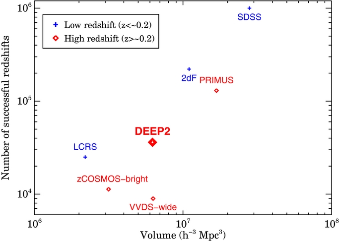
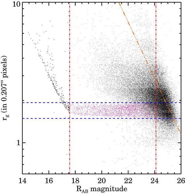
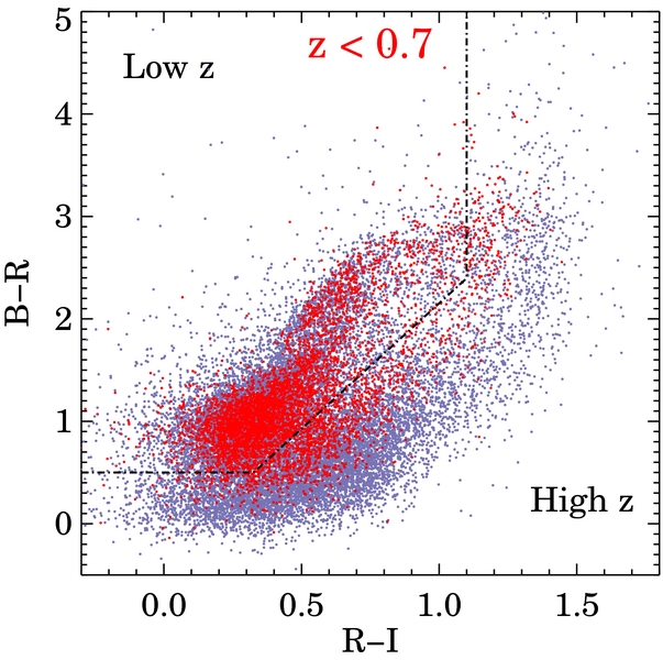
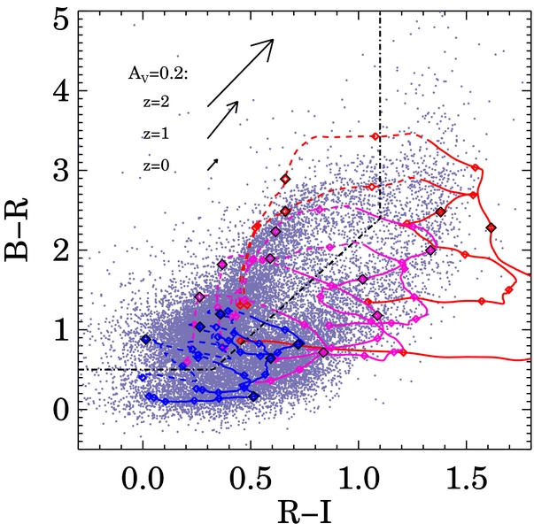
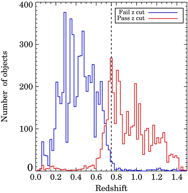
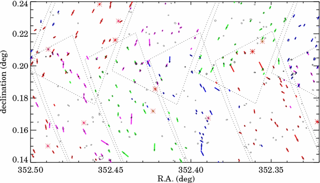
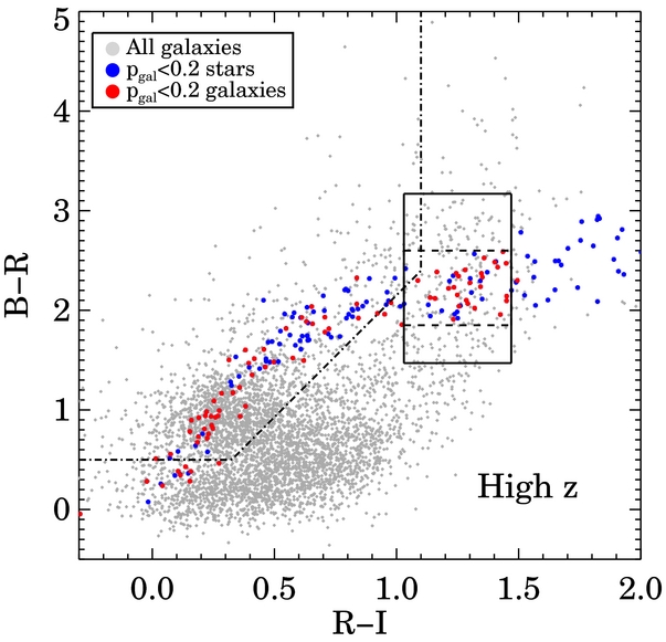
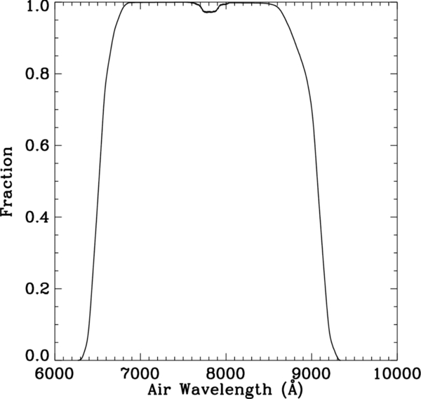
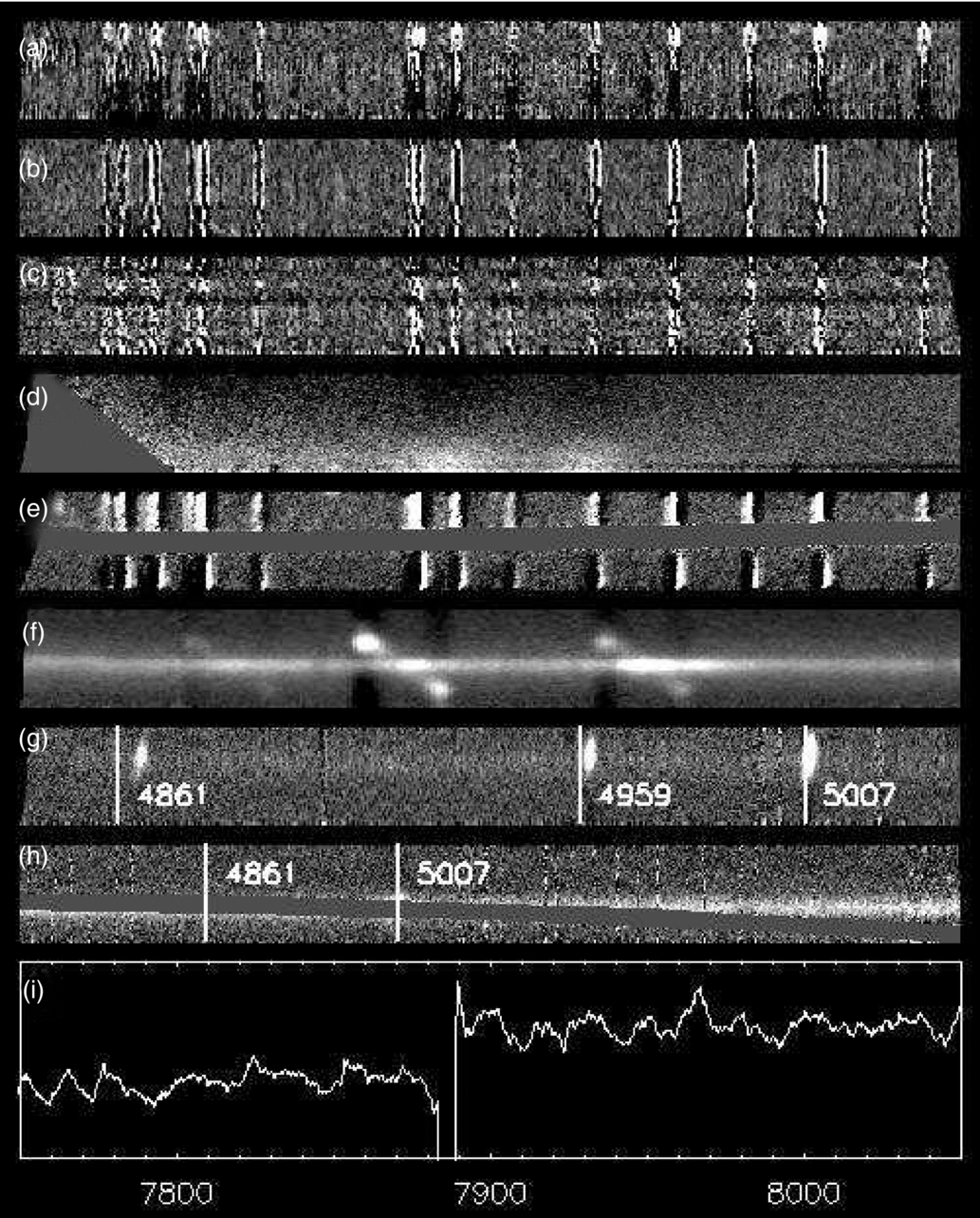
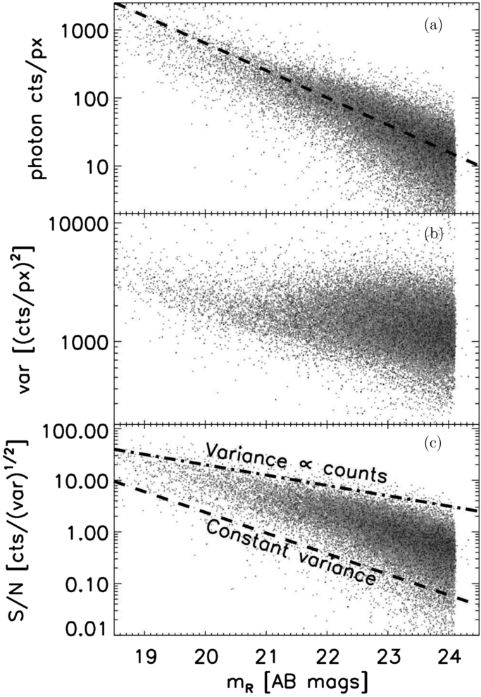
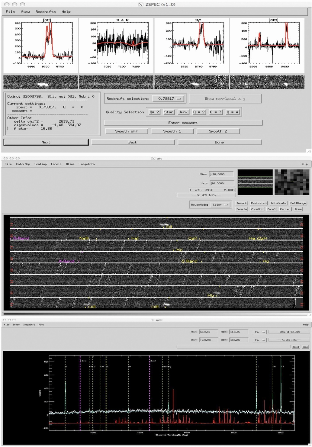
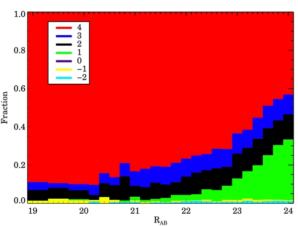
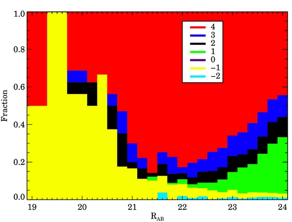
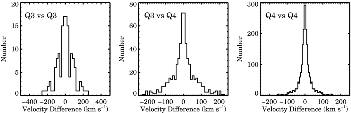
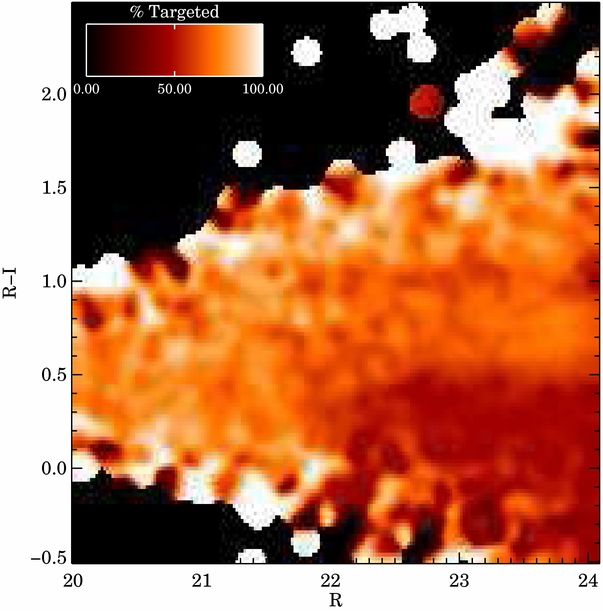
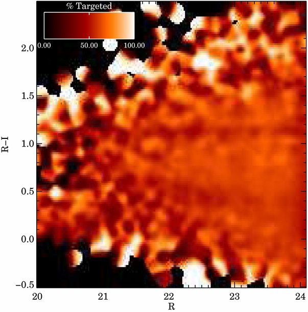
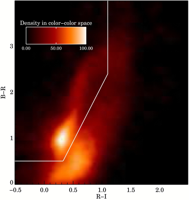
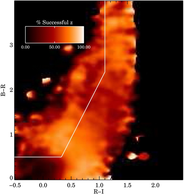
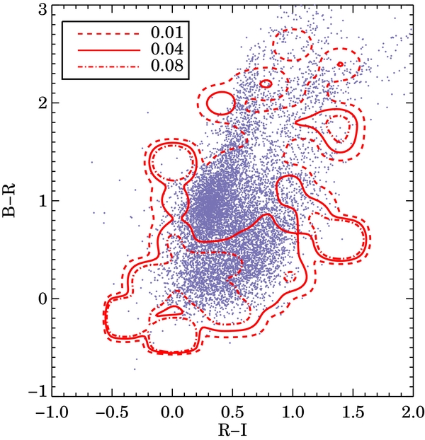
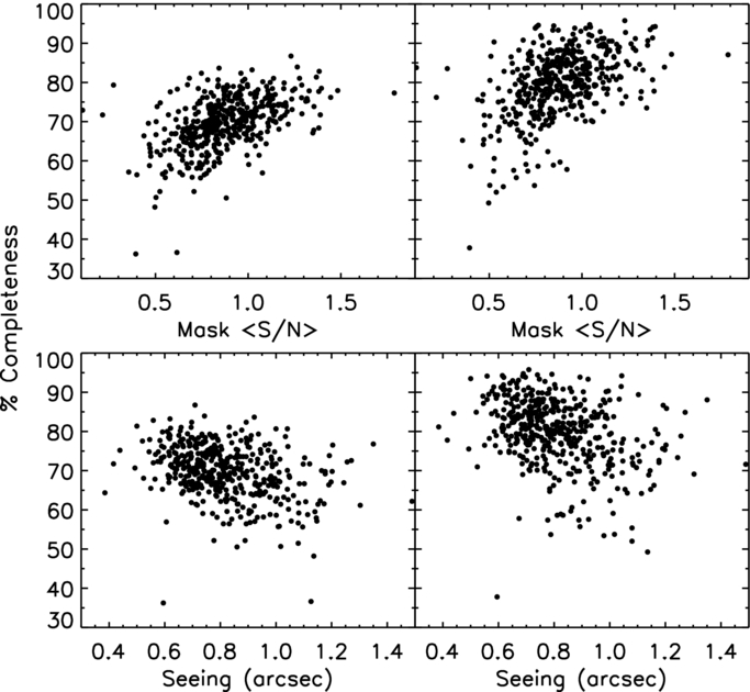
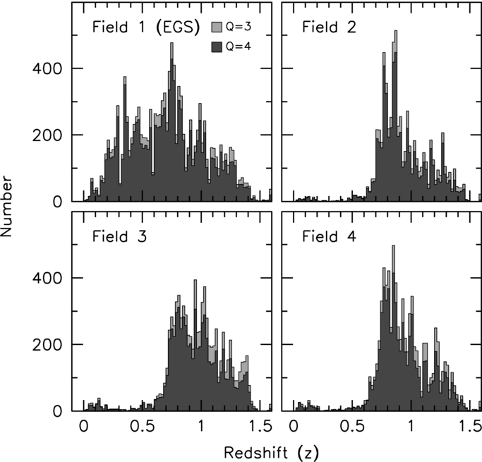
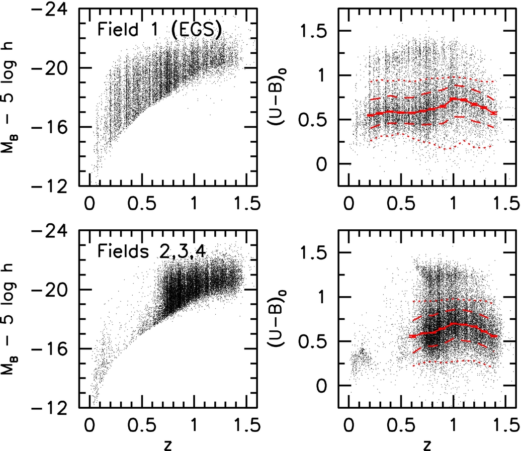
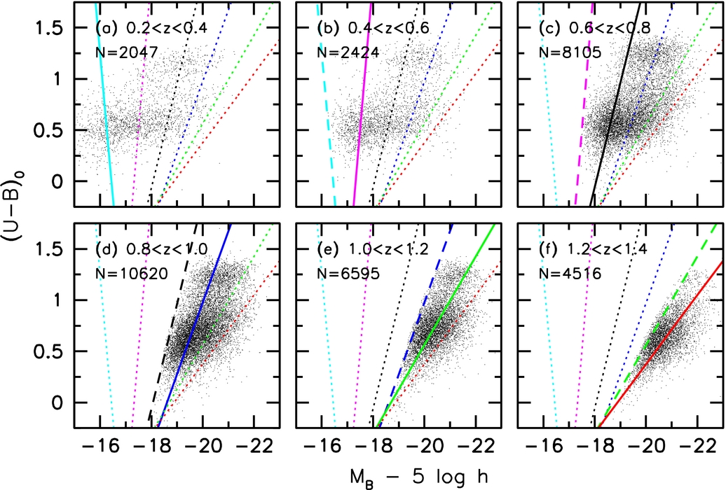