


ABSTRACT
Advanced image processing of Large Angle and Spectrometric Coronagraph Experiment (LASCO) C2 observations reveals the expansion of the active region closed field into the extended corona. The nested closed-loop systems are large, with an apparent latitudinal extent of 50°, and expanding to heights of at least 12 R☉. The expansion speeds are ∼10 km s−1 in the AIA/SDO field of view, below ∼20 km s−1 at 2.3 R☉, and accelerate linearly to ∼60 km s−1 at 5 R☉. They appear with a frequency of one every ∼3 hr over a time period of around three days. They are not coronal mass ejections (CMEs) since their gradual expansion is continuous and steady. They are also faint, with an upper limit of 3% of the brightness of background streamers. Extreme ultraviolet images reveal continuous birth and expansion of hot, bright loops from a new active region at the base of the system. The LASCO images show that the loops span a radial fan-like system of streamers, suggesting that they are not propagating within the main coronal streamer structure. The expanding loops brighten at low heights a few hours prior to a CME eruption, and the expansion process is temporarily halted as the closed field system is swept away. Closed magnetic structures from some active regions are not isolated from the extended corona and solar wind, but can expand to large heights in the form of quiescent expanding loops.
Export citation and abstract BibTeX RIS
1. INTRODUCTION
Recent advances in observations of the corona are leading to increasingly complicated and accurate models of the connection between the Sun, the corona, and the solar wind. Antiochos et al. (2012) give a detailed description of current efforts to unify models of magnetic field structure in the low corona with the observed properties of the heliospheric solar wind, and give fresh definitions of the two types of solar wind (traditionally named slow and fast) according to three sets of properties based on location, time variability, and composition. The slow solar wind has high variability in speed, density, and composition, and there is not yet a single model that describes its origins and explains all its observable characteristics in a unified manner.
Uchida et al. (1992) discovered the continuous expansion of active regions into the corona using Yohkoh soft X-ray observations. They found occasional or continuous expansion of closed-field active regions with speeds of a few km s−1 to a few tens of km s−1 not associated with reconnection. At the time, their findings were contrary to the established model of active regions as stable regions of magnetohydrostatic equilibrium. Despite this important result, the expansion of active region closed-field regions to great heights to directly form part of the slow solar wind has not been generally accepted, probably due to the lack of observational evidence for such expansion in the extended inner corona (X-ray and extreme ultraviolet (EUV) emission decreases steeply with height). Typically, modeling efforts of active region emerging flux and interaction with coronal fields concentrate on eruptive scenarios (e.g., Hood et al. 2012). There are also many observational studies of bulk plasma flow within active regions, with some of this flow being interpreted as forming part of the slow wind along open field lines (e.g., Baker et al. 2009; Harra et al. 2008). Some studies have invoked the expansion of active regions as a driver of outflow at the periphery of active regions (Murray et al. 2010), but do not include the active region expansion as a direct contribution to the solar wind. There have been some efforts to interpret heliospheric in situ magnetic field measurements in terms of expanding closed-field regions (Gopalswamy et al. 2013), and several studies that map in situ measurements to the Sun have linked slow wind flows directly to active regions (Kojima et al. 2000; Neugebauer et al. 2002). Without direct observations in the extended inner corona (i.e., in coronagraph observations), such links remain speculative.
Sheeley & Wang (2007) showed that the bases of helmet streamers (which often lie above active regions) could experience a period of expansion, followed by a rapid event that results in the ejection of a plasmoid and a contraction of the streamer base ("in–out pairs"). Their parameter study for a model streamer (a simple dipole and current sheet) showed that the expansion and subsequent reconnection were sensitive to the rate of magnetic field replenishment at the base of the system. Indeed, the closed-loop system could expand to large heights without subsequent reconnection and contraction given sufficient replenishment of the closed field at the base. Their study, however, discussed the expansion of helmet streamer bases in terms of a build-up to reconnection and an eruptive event rather than a steady-state process.
New image processing techniques can reveal new phenomenon in the data. In particular, it is possible to effectively separate the dynamic and quiescent components of coronagraph images (Morgan et al. 2006, 2012), and thus reveal faint details of moving features. This paper briefly describes the new processing techniques in Section 2. A detailed description of a set of expanding loops is given in Sections 3.1–3.4, followed by a briefer description of another set in Section 3.5, followed by discussion, conclusions, and ideas for future work in Section 4.
2. DATA PROCESSING
The Large Angle and Spectrometric Coronagraph Experiment (LASCO) C2 coronagraph (Brueckner et al. 1995) has observed the extended inner corona in visible light for almost 17 yr. The level 0.5 fits files of the normal observation mode is used for this study (these are the most frequent observation using the orange filter without polarization measurements). The aim of the data processing is to apply the quiescent–dynamic separation method described in Morgan et al. (2012). After removing long-term minimum backgrounds from the images, the normalizing-radial-graded filter (NRGF; Morgan et al. 2006) is applied, which removes the steep radial drop in brightness. The resulting images contain slow-changing quiescent coronal structures (i.e., streamers and coronal holes) that are close to radial in structure within the LASCO C2 field of view (FOV), and dynamic events which are generally non-radial and, by definition, change rapidly compared to the quiescent structures. The quiescent and dynamic components can be separated by applying deconvolution along the radial and time dimensions of a time-series of images, which gives a set of images that contains only noise and dynamic coronal events, with the quiescent structure removed.
This method is superior to the more commonly used one of running difference images for several reasons. Noise is inherently amplified by time-differencing, and the resulting dynamic features, although effectively revealed, contain positive and negative regions depending on the activity in the previous (subtracting) image—this makes interpretation more difficult. The quiescent–dynamic separation by deconvolution removes most of the quiescent structure by exploiting the smoothness of the quiescent structure in the radial direction, thus noise is not inherently amplified. Edge-enhancement methods (including wavelet-based methods) enhance edges and high spatial frequency features within coronagraph images, but this applies equally to both the quiescent and dynamic structures (as well as noise). They are therefore not the best methods to study dynamic structures in isolation. The usefulness of the quiescent–dynamic separated images to study the structure and kinematics of coronal mass ejections (CMEs) is shown in more detail in Byrne et al. (2012). For coronagraphs, no other current method can reveal such faint detail of the dynamic corona with such clarity.
Over two months of data collected at the start of 2011 is processed and analyzed. As other instruments aboard Solar and Heliospheric Observatory (SOHO) have failed, the telemetry rate for LASCO has improved. In early 2011, the observational cadence of the C2 coronagraph was on average around 12 minutes, with only occasional data gaps of longer than a few hours. This was a rising period of activity where there were plenty of active regions but CMEs were not occurring very often, allowing long enough time periods to study faint dynamic structures. Other observation-based information used in this work includes: active region summary data from the Solar Region Summary archive (see Acknowledgements); Mauna Loa Solar Observatory (MLSO) MK IV coronameter data (Fisher et al. 1981); images from the Atmospheric Imaging Assembly (AIA; Lemen et al. 2012) and the Helioseismic and Magnetic Imager (HMI; Scherrer et al. 2012) aboard the Solar Dynamic Observatory (SDO; Pesnell et al. 2012); and images from the Extreme UltaViolet Imager (EUVI)—part of the Sun Earth Connection Coronal and Heliospheric Investigation (SECCHI; Howard et al. 2002) aboard the Solar Terrestrial Relations Observatory (STEREO; Kaiser 2005).
3. RESULTS
3.1. Context
Figure 1 shows a composite image of the corona at 2011 March 1. In the east corona, there is a large system of streamers, with four or five main bands of higher brightness distributed between angles approximately 20° south to 45° north of the equator. Further information on the coronal structure during this time is gained by applying Quantitative Solar Rotational Tomography (see Morgan et al. 2009) to LASCO C2 data, which results in the map in Figure 2(a). The dotted line in the map shows the portion of the corona directly above the east limb on 2011 March 1. There is a reasonable correlation between the complicated multi-streamer structure in the east corona suggested by the LASCO image of Figure 1 and the density distribution of the tomographical map at the same position. The northernmost mid-latitude streamer in the east is the largest high-density structure, being a narrow longitudinally extended high-density sheet that is probably associated with the current sheet. At the position of the limb, this sheet splits into two distinct density sheets—this splitting can be seen in the LASCO image. Some of these high-density sheets must be pseudostreamer structures (Wang et al. 2007, 2012). The southernmost density structure at the east limb is ∼10° south of the equator, but appears more southerly in the LASCO image due to projection of the density structure at longitude 135°. Potential field source surface models reveal that the current sheet is approximately parallel to the east limb as it descends from north to south during 2011 March 1.

Figure 1. The corona observed at times close to 2011 March 1 19:30 by AIA/SDO at 171 Å (inner corona), MLSO MKIV coronagraph (middle corona), and LASCO C2 (outer corona). All off-limb regions have been processed using the NRGF (Morgan et al. 2006).
Download figure:
Standard image High-resolution image
Figure 2. (a) Longitude–latitude tomographical map of the corona at a height of 4 R☉ made using LASCO C2 observations over half a solar rotation (∼two weeks). The red is highest density and the white regions are those masked to zero since they do not contain any significant high density structures. The dotted (dashed) line shows the position of the east (west) limb at 2011 March 1 19:30 (corresponding to the image of Figure 1). The tomographical process is described in Morgan et al. (2009), with the added improvement of using the separated quiescent-component images (see illustration of this step in Morgan 2011). These maps are useful to show the distribution of the more stable, large streamers in the corona, while the very small-scale features in the map must be treated with care since they are more likely to be a consequence of data errors or rapid changes in the corona which disrupt the tomographical process. (b) Helioseismic and Magnetic Imager (HMI/SDO) synoptic map for Carrington rotation 2107. The dotted (dashed) line shows the position of the east (west) limb at 2011 March 1 19:30. The circled active region is at the west limb during 2011 March 8, and is relevant to Section 3.5.
Download figure:
Standard image High-resolution image3.2. Expanding Loops
On the solar disk close to the east limb are a group of large active regions, as shown in the HMI synoptic map in Figure 2(b). These active regions are responsible for several small and large CMEs over an extended time period. A small, faint and slow CME passes through the C2 FOV at the start of 2011 March 1 at the position of the northernmost east streamer. As the CME propagates, a large loop that is centered at the east equator expands slowly into and through the C2 FOV. The small CME and initial loop are precursors to a nested systems of loops which expands into the corona over a period of almost three days. This is a period of stability in the east where there are no sizeable eruptions for approximately 63 hr. Figure 3 shows images of the east–north–east corona taken over this period starting 2011 March 1 06:20. These images (and the associated movie in particular) clearly show a system of loops expanding outward through the FOV of LASCO C2. For the first ∼10–15 hr, the loops are centered just a few degrees north of the equator. They then move slightly northward and by the end of the sequence are centered at the position of the most northerly streamer (about 10° north of the equator).

Figure 3. Selected set of 25 observations starting at 2011 March 1 06:20 (top left) and ending at 2011 March 3 21:22 (bottom right), showing a series of expanding loops in the east corona. The inner field of view is at 2.2 R☉. The region extends from −5.3 to −1.4 R☉ in the x direction and −1.4 to 3.5 R☉ in the y direction. The time increment between each displayed observation is just over 2 hr on average (the true observational cadence is ∼12 minutes). The order is row-major (left to right, then top to bottom). The sequence ends with the appearance of a bright CME and ray (bottom right).(An animation of this figure is available in the online journal.)
Download figure:
Standard image High-resolution imageFigure 4 shows the position of the initial loop overlaid on a LASCO C2 image. The loop expands to a very large size. By the time the loop extends throughout the C2 FOV (or with apex height close to 6 R☉), the position-angle separation of the loop legs is over 50°, or a plane-of-sky separation of over 2 R☉. At this time, the loop bridges several quiescent streamer structures. That is, the loop is not part of a large individual helmet streamer, and because it spans a system of separate radial streamers is unlikely to be embedded directly within the quiescent streamer structure. The same is true of the whole system of expanding loops shown in Figure 3—they are not limited in spatial extent to one individual streamer structure. Unfortunately, it is impossible using current observations to estimate the true three-dimensional position of the expanding loop. If it is not part of the main streamer structure, then the tomographical map of Figure 2(a) suggests it must be positioned somewhere in the space between high-density streamers at approximately longitude 90°, latitude 30°. This space is centered at the east limb, and lies close to the active region at longitude 90°, latitude 10°–20°.

Figure 4. The position of the initial expanding loop overlaid on a LASCO C2 image for 2011 March 1 15:35.
Download figure:
Standard image High-resolution imageFigure 4 illustrates just how faint these loops are. The first initial loop is by far the most clear and bright loop found in this data set—parts of it can even be seen in standard running-difference images of the type often used for CME studies. It cannot be seen in images that have not been processed specifically to reveal dynamic features. The loop systems that follow this initial loop are somewhat fainter and can only be seen in the dynamic-separation images (see Figure 3). Their signal is close to the noise level, fainter than the faintest CMEs. The only reason they are seen is due to their large size and coherent loop-like structures in the dynamic images. Running-difference images do not show these fainter loops due to the relative increase of noise caused by the subtraction, the narrow profile of the loops, and possibly due to their slow propagation.
The height–time plot of Figure 5 is taken at the east equator during the times corresponding to the sequence shown in Figure 3. The loops are clearly seen as curved enhancements, the faintest of which tend to blur into the noise at increasing heights (above ∼5 R☉). New loops appear and expand every three or four hours, and they all have a similar curved height–time profile indicative of acceleration. Examination of these curves reveals a speed of ∼20 km s−1 at 2.5 R☉, increasing to 60 km s−1 by 5 R☉, with an uncertainty of around ±10 km s−1. These values are comparable to those of Uchida et al. (1992), who find velocities on the order of 10 km s−1 at heights of 1–1.5 R☉.

Figure 5. Height–time plot of intensity along the radial slice lying within 2° of position angle 90° (east equator). The expanding loops are seen as ridges of enhanced brightness. They are traced by eye until the signal is lost at large height. This plot corresponds to the first two rows of images in Figure 3. There is a ∼2 hr data gap at 2011 March 1 18:00.
Download figure:
Standard image High-resolution image3.3. Source of the Loops
As is common to all current studies of the corona, the lack of coronagraph data below the FOV of LASCO C2 is a large hindrance to tracing the source of the loops. This introduces large uncertainty in stating any link between the expanding loops and events closer to the Sun. There is, however, a plausible source for the loops, and this is the active region at longitude 90°, latitude 10°, seen in the HMI synoptic map of Figure 2(b) for Carrington rotation (CR) 2107, and which is close to the east limb during 2011 March 1. It is not present in the HMI synoptic map for the previous CR. Figure 6 shows a daily series of EUVI/SECCHI-STEREO B 195 Å observations starting on 2011 February 25. The active region first appears sometime during 2011 February 25 and increases in size from day to day until it reaches the position of the east limb in the LASCO C2 reference on 2011 March 1 and 2011 March 2 (this is approximately the center of the disk for STEREO B). Movies made from EUVI-B observations show a flurry of activity in the core of the active region at the same time as the appearance of the expanding loops—this includes rapid brightening of small loops, rapid movement of small structures probably related to reconnection, and possible flux emergence. Uchida et al. (1992) describe similar small-scale activity related to expanding active regions.

Figure 6. Six EUVI SECCHI/STEREO B observations taken at 00:05 daily between 2011 February 25 and 2011 March 2, with time increasing from top left to bottom right (row-major). These are 195 Å images showing the portion of the corona containing the newly emerging active region. The first obvious appearance of the active region is shown with the white arrow in the second panel.
Download figure:
Standard image High-resolution imageHigh time-resolution AIA/SDO observations of the active region above the east limb during 2011 March 1 through 2011 March 2 show loops expanding from the central region, seemingly either to disappear with increasing height or to pass from the AIA FOV. It is very difficult to make direct connections between the expanding loops seen in LASCO and the activity at the base of the loops, and only one clear case is found. An expanding loop is shown in Figure 7. This particular loop becomes the first clear loop seen in the first few frames of Figure 3 at extended coronal heights. In the AIA data, the approximate expansion speed at low heights is 10 km s−1.

Figure 7. Short sequence of AIA/SDO 171 Å images showing one particularly clear case of an expanding loop.
Download figure:
Standard image High-resolution imageFigure 8 shows the estimated temperature of the low corona for the east limb active region and surrounding areas for 2011 March 4 00:00. The temperatures are estimated from the multi-wavelength bandpass data of AIA/SDO, using a method similar to that of Aschwanden et al. (2013). The method used to constrain the temperature is least reliable for off-limb regions (due to the extended line-of-sight). It is obvious that the active region shows localized hot regions at its base, probably highlighting regions of high activity and/or flux emergence. The apexes of some of the loops reach temperatures of over ∼2 MK, with an extended line of high temperature tracing the peaks of several loops.

Figure 8. AIA/SDO 171 Å image (left) and corresponding temperature map (right) of the low corona for 2011 March 4 00:00. The colors correspond to the log temperatures shown in the colorbar on the right.
Download figure:
Standard image High-resolution image3.4. Disruptions by CMEs
Figure 9 shows the loop system prior to the CME that effectively brings to an end the first set of quiescent loop expansions. This sequence clearly shows that the CME erupts from the same position as, and with a similar shape to, the loops. They presumably therefore arise from the same source region. As clearly seen in the figure, there is a bright, non-radial ray at latitude ∼45° which starts to brighten from the base upward up to 2 hr prior to the appearance of the main CME front. The lowest loops in the C2 FOV also start to brighten around 2 hr before there is an obvious CME. Accompanying the brightening, the low loop expands slightly, rising slowly into the C2 FOV at a slow speed similar to that of the previous quiescent expanding loops. Finally, the CME front erupts into the C2 FOV, destroying the quiescent system of nested loops which lie in its path. This disruption is only temporary since the loop system emerges in the wake of this CME, approximately six hours after the first appearance of the CME. Figure 10(a) shows the main body of the first CME. In its wake is a complicated network of non-radial lines and blobs which gradually propagate outward and/or disappear (Figure 10(b)). Figure 10(c) shows the corona as the CME wake has mostly disappeared from view, and just as a second CME is appearing as a bright loop immediately south of the equator. The re-emergence of the nested loop system is apparent in Figure 10(c). By the time the second CME, seen in whole in Figure 10(d), has exited the FOV, another CME is propagating at the position of the expanding loops. This CME is shown in Figure 10(e). It is extremely faint, at the same kind of brightness level as the expanding loops, and shows a classic flux tube and leg-reconnection signature in its structure. The extremely faint CME shown in Figure 10(e) makes its first appearance in the C2 FOV at around 2011 March 4 06:00. Its height–time profile is very similar to that of expanding loops, and its brightness is also similar (i.e., extremely faint). This faint CME does not seem to disrupt the expanding loop system, and they continue until ∼2011 March 5 06:00.

Figure 9. Time series of dynamic-component LASCO C2 images. The time increment is 12 minutes (i.e., the observational cadence of LASCO C2), starting at 2011 March 3 20:34. Each frame is a polar-coordinate image showing a portion of the dynamic corona between position angles 30°–130° (horizontal axis) and heights 2.2–6 R☉ (vertical axis). The whole sequence covers three hours of observation. Note that the image contrast is optimized to show the faint loops, so that the bright CME front in the last few panels is saturated.
Download figure:
Standard image High-resolution image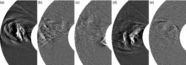
Figure 10. Several LASCO C2 dynamic images showing CME activity for observation times (a) 2011 March 3 23:58, (b) 2011 March 4 03:21, (c) 05:45, (d) 06:57, and (e) 15:32.
Download figure:
Standard image High-resolution image3.5. Another Example
Figure 11 shows another example of a system of expanding loops. This system lies above an active region on the west limb, circled in white in the HMI synoptic map of Figure 2(b). These loops form and trace the shape of an underlying large helmet streamer, as can be seen in Figure 12, and seem to be part of or embedded within the streamer. This is a key difference to the loops of the main example of Figure 3. These loops are of a similar size to the previous set, if a little narrower in position angle. They are slightly brighter but still very faint compared to the background streamer. The system rises after the passage of a very faint CME, labeled A at 2011 March 7 00:11. Faint brightenings in small loops, labeled B and C, lead to small outward-propagating blobs that appear at the apex, labeled D. The shape of these small loops (apex heights at around 3.5 R☉) is clearly more pointed, less rounded, than the shape of the previous expanding loops. In fact, the pointed shape and the fact that the converging legs do not always seem to meet at an apex in a clean loop shape suggests that this may well be a direct observation of helmet streamer interchange reconnection at the apex of the closed field in a helmet streamer. This is supported by the appearance of an outward propagating small blob labeled D. Such interchange reconnection provides a mechanism for an active region to exchange flux with neighboring open field regions (see Wang 2012, for example).
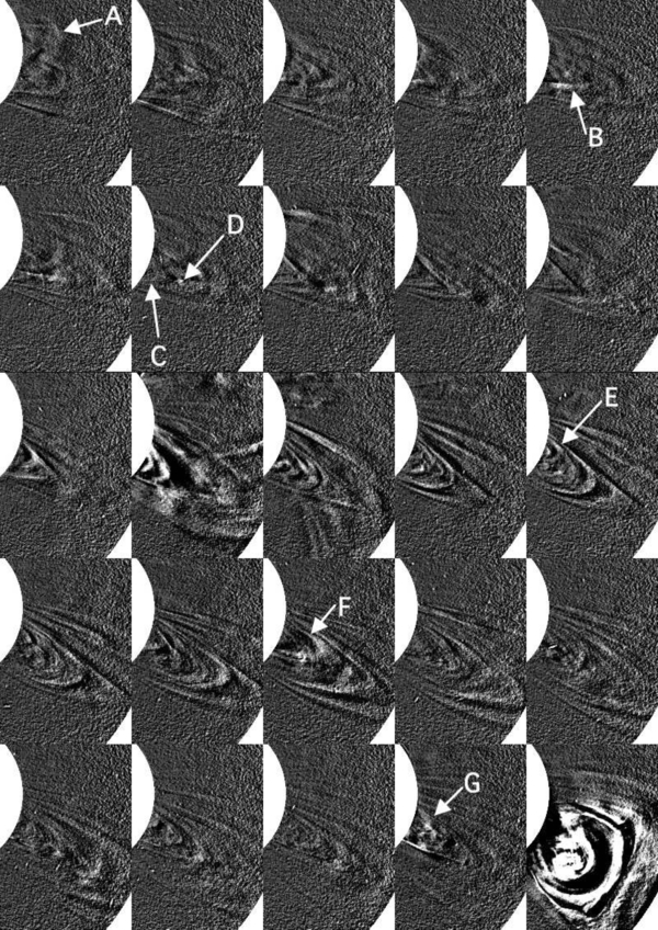
Figure 11. Same as Figure 3, but for period beginning 2011 March 7 00:11 (top left) and ending at 2011 March 8 21:18 (bottom right), showing a series of expanding loops in the west corona. The region extends from 1.56 to 5.3 R☉ in the x direction and −3.9 to 1.4 R☉ in the y direction. The time increment between each displayed observation is 108 minutes on average. The sequence ends with the appearance of a bright CME. Note that the last frame showing the main CME has the same high image contrast enhancement as the previous frames and is therefore saturated.(An animation of this figure is available in the online journal.)
Download figure:
Standard image High-resolution image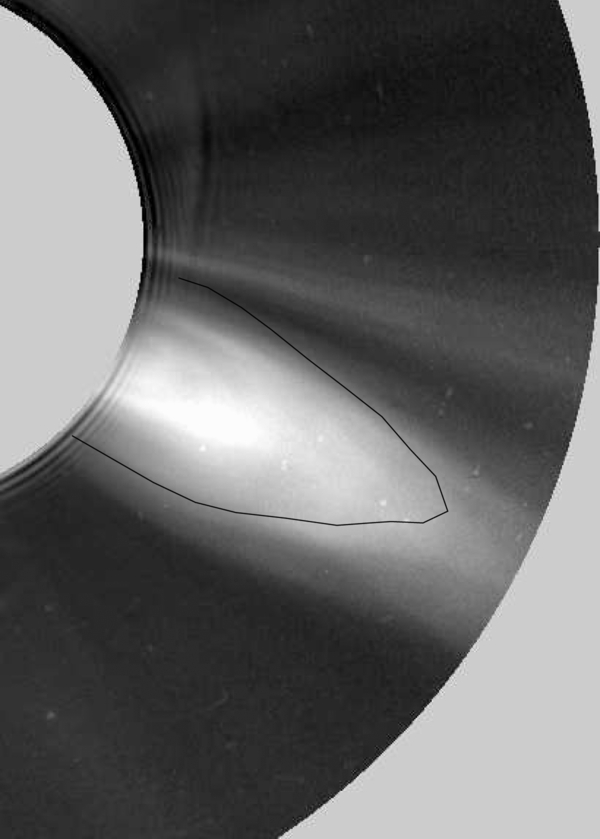
Figure 12. The position of one of the expanding loops shown in Figure 11 overlaid on a LASCO C2 image for 2011 March 8 08:44.
Download figure:
Standard image High-resolution imageIn the 12th frame, a large CME north of the west equator disrupts the helmet streamer and seems to trigger brightenings in the loop system. The shape of the loops then becomes more rounded, and more similar to the previous set of expanding loops of Figure 3. By the frame labeled E, the nested system of expanding loops is very clear, but rather complicated. The northernmost legs of the loops are bunched together, and within the larger loops the smaller loops at the lowest heights are rather unclear and distorted. This may be a line of sight effect rather than an intrinsic structural complexity. By the frame labeled F, the loops are simpler in structure. The system is large, and extends past the 6 R☉ outer FOV of LASCO C2. To both sides of the closed loop system are similarly aligned narrow rays which may be the legs of loops that have already expanded out of the FOV. The series comes to an end with the eruption of a large CME as shown in the last frame. The system of loops brightens around two hours or more prior to the eruption of the main CME. This brightening is labeled G in the penultimate frame. This set of expanding loops is accompanied by a swelling in the size of the helmet streamer. This swelling is apparent in the original LASCO images (i.e., without dynamic separation), and is typical of many helmet streamers prior to a large CME.
The loops are bright enough during 2011 March 8 to be seen in the LASCO C3 FOV. Figure 13 shows a time series of LASCO C3 dynamic-component images, clearly showing loops expanding out to a height of at least 12 R☉. Unfortunately the dynamic signal becomes dominated by noise beyond this height and it becomes impossible to determine the fate of the expanding loops at larger heights.

Figure 13. Same as Figure 11, but for period beginning 2011 March 8 12:50 and ending at 2011 March 8 14:12, showing the same series of expanding loops in the west corona but in the LASCO C3 field of view. The region extends from 3.5 to 13.5 R☉ in the x direction and −9.9 to 3.6 R☉ in the y direction. The white contour is at a height of 12 R☉.
Download figure:
Standard image High-resolution image
4. DISCUSSION AND CONCLUSIONS
There is no topological reason forbiding the expansion of closed loops into the extended corona. The main physical argument that makes such large loops puzzling is the stability of the closed-field system for such long periods at such large heights, particularly when dragged out to large heights by the plasma expansion into the solar wind. The appendix to Sheeley & Wang (2007) suggests that a sufficient replenishment of the closed field at the streamer base may allow and sustain the expansion of closed loops to large heights without reconnection and collapse. The AIA/SDO images presented in this paper for the first case of expanding loops support this view, by showing continuous emergence and expansion of small loops in the low corona between the legs of the large expanding loops. Due to the complexity of the region, and lack of observations above the AIA FOV, it is unclear whether these smaller loops reconnect with systems of neighboring loops to form larger loops, or whether they somehow expand directly to form larger coronal loops. The coherence of the loops during expansion would suggest the latter. Uchida et al. (1992) came to similar conclusions for active region expansion observed at lower heights.
The second example of expanding loops shown in Section 3.5 is considerably different from the first example of Sections 3.1–3.4. The streamer of the second example is a helmet streamer, with the corresponding current sheet seen edge-on (i.e., the high-density sheet is aligned along the line of sight). The expanding loops are largely confined to within the streamer. The first example of loops seems to lie across a large fan-like system of narrow radial streamers. Such a fan-like system is expected as the heliospheric current sheet, and/or pseudostreamer sheets, are aligned perpendicular to the line of sight. It is not possible to say whether the expanding loops are embedded within this system, or simply share the same region of the image along the line of sight. One argument for the latter case is that the loops are coherent in their expansion. If they were embedded within the streamer sheet, and some parts of the sheet are denser than the others, the shape and expansion of the loops would be influenced by this underlying structure.
The systems of expanding loops presented here are a different phenomena than the CME-like flux rope phenomenon of Sheeley et al. (2009; Sheeley blobs). From the appearance of the blobs from the side (as opposed to edge-on), they describe the flux ropes as diffuse arches. However, their arches are very long flux ropes, and lack a clean loop-like structure. Neither do the blobs they describe show the nested expanding loop structure revealed here, although the blobs can occur at a rate of around four a day. This is less frequent and regular than the expanding loops. The outflow speed of Sheeley blobs is more than double what is measured for the expanding loops at 5 R☉, and the Sheeley blobs are considerably brighter, being on the order of 10% of the brightness of the host streamer. By identifying the pixels containing the brightest loops in the dynamic images shown for the helmet streamer of Section 3.5, and comparing the values in these pixels to the original images, the brightness of the expanding loops is around 3% of the background streamer.
Wang & Sheeley (2006) found evidence of expanding loop systems in the context of a build-up toward reconnection and the ejection of a helical flux rope, followed by the collapse of the loop system, and showed that the expansion and reformation of the streamer occurred at slightly different locations due to flux emergence below one of the streamer legs. Sheeley & Wang (2007) made an extended study of several similar cases. Applying the processing of this work to the example they give of a system of expanding loops from 2004 January 20 in the northeast corona reveals a large system of expanding loops which existed at least 66 hr prior to the collapse of the system on 2004 January 20 06:00 (around twice the time period found using time-differencing). A smaller system of loops at the equatorial leg of the loops actually contracts inward around 24 hr prior to the collapse of the system, and the actual collapse seems linked to this contraction, suggesting that the reconfiguration that leads to the end of the expanding system may not be linked to the large halo CME at the start of 2004 January 20 as previously thought. Systems of expanding loops may often (or always) be disrupted or destroyed by reconnection at large heights ("in–out" pairs or blobs) or catastrophic events from active regions (CMEs), but the fact that they exist for such long periods suggests that they are a natural quiescent process above regions of flux emergence on the Sun, and should not be interpreted solely in terms of a build-up to an eruptive event. Indeed, the main example described in this work shows that after the passage of a large CME, the disruption to the expanding loop system is temporary, with a renewed period of quiescent expansion for around 24 hr following the CME.
That closed magnetic loops are expanding into the extended corona from active regions has important implications for interpretation of in situ solar wind measurements. Several works have mapped solar wind streams to active regions (e.g., Kojima et al. 2000; Neugebauer et al. 2002 and references within), but such results are subject to mapping uncertainties, or to the uncertainties of potential field models which map the extended corona to features at the Sun. Our results show direct evidence of the active region closed field expanding into the solar wind. In discussing the possible heliospheric signature of expanding loops compared to signatures of interplanetary CMEs, Gopalswamy et al. (2013) states that the expanding loops should not carry a signature of high charge states since they have not experienced reconnection or a flare process. Our analysis of AIA/SDO observations of the active region underlying the expanding loop systems show that some of the loops are hot, at around ∼2 MK or higher. This ionizes iron to 14–16+, which could account for some high-charge state measurements in the heliosphere. Expanding loops may also provide a partial explanation for the variable nature of the slow solar wind. The background streamers have an extended structure along the line of sight, while the expanding loops are probably narrow structures. Therefore, even though their brightness is only around 3% of the background streamers, their relative density may be considerably higher. In truth, it is unknown whether these slow and dense closed-field features carry a signature out to the heliosphere as variations to the background, continuous slow wind. This depends on their heliospheric evolution and the frequency of their occurrence, which will be studied in a future work.
Future studies of expanding loops should aim to discover the true source of the loops at the Sun. Where exactly are the loop legs at the disk? An observational study combined with suitable MHD models would help in this and other respects. This initial study should also be extended to a long time period to establish how common such loops are, and also to see if there is a correlation between systems of expanding loops and subsequent CMEs. Given appropriate processing of coronagraph data, evidence of small-scale dynamic activity and small loop expansion can be seen at almost all times in the corona, and a more detailed study of this activity would be a direct observational study of the main source of the slow solar wind and the relationship between active regions and the extended corona. Our findings demand a revision of current models, and inclusion in interpretations of many coronal and heliospheric observations.
The authors are indebted to an anonymous referee whose valuable suggestions greatly improved this work. Huw is grateful for funding from the Coleg Cymraeg Cenedlaethol to Prifysgol Aberystwyth and the support of SHINE grant 0962716 and NASA grant NNX08AJ07G to the Institute for Astronomy, University of Hawaii. Lauren and Drew are supported by STFC studentships to Prifysgol Aberystwyth. The SOHO/LASCO data used here are produced by a consortium of the Naval Research Laboratory (USA), Max-Planck-Institut für Aeronomie (Germany)), Laboratoire d'Astronomie (France), and the University of Birmingham (UK). SOHO is a project of international cooperation between ESA and NASA. The STEREO/SECCHI project is an international consortium of the Naval Research Laboratory (USA), Lockheed Martin Solar and Astrophysics Lab (USA), NASA Goddard Space Flight Center (USA), Rutherford Appleton Laboratory (UK), University of Birmingham (UK), Max-Planck-Institut für Sonnen-systemforschung (Germany), Centre Spatial de Liege (Belgium), Institut d'Optique Théorique et Appliqúee (France), and Institut d'Astrophysique Spatiale (France). The active region data is extracted from the Solar Region Summary reports, prepared jointly by the US Dept. of Commerce, NOAA, Space Weather Prediction Center and the US Air Force from data received by the Space Weather Operations branch of NOAA.