


ABSTRACT
We present high-resolution CO J = 3–2 maps of the Galactic center region, taken with the ASTE 10 m telescope. We have collected approximately 30,000 spectra with a 34'' grid spacing. The mapping area is roughly −1 8 < l < +35 and −08 < b < +09, which includes the central molecular zone and Bania's Clump 2, covering almost the full extent of the molecular gas concentration in the Galactic center. These CO J = 3–2 images show a behavior similar to the CO J = 1–0 images with the same resolution. Molecular gas in the Galactic center shows a higher J = 3–2/J = 1–0 intensity ratio (∼0.7) than the gas in the spiral arms in the Galactic disk (∼0.4). The CO J = 3–2/CO J = 1–0 luminosity ratio is 0.71. We see several regions with very high J = 3–2/J = 1–0 intensity ratios exceeding 1.5, including the Sgr A, l = +13, l = −04, and l = −12 regions. A number of small spots of high ratio gas are also found. Many of them have large velocity widths, indicating that they are spots of hot molecular gas shocked by unidentified supernovae and/or winds from massive stars.
Export citation and abstract BibTeX RIS
1. INTRODUCTION
Many galaxies contain huge amounts of molecular gas in the few hundred parsecs from their centers (Mauersberger & Henkel 1993). This concentration of molecular gas provides the raw ingredients for star formation and, in many cases, can be a potential fuel reservoir for the central activity. Our Galaxy also has a concentration of molecular gas (Morris & Serabyn 1996), often referred to as the "central molecular zone (CMZ)." Thus far, several molecular line surveys have been performed for the CMZ (e.g., Jones et al. 2012, and references therein). Molecular gas in the CMZ is higher in temperature and density than that in the Galactic disk and shows highly complex distribution and kinematics as well as a variety of peculiar features (e.g., Oka et al. 1998b, and references therein). Molecular clouds in the CMZ generally have large velocity widths as well as a larger virial theorem mass compared with the mass derived from the CO luminosity (Oka et al. 1998a, 2001b). The widespread SiO emission in the CMZ has been attributed to an interstellar shock (Martín-Pintado et al. 1997; Hüttemeister et al. 1998). The ubiquity of complex organic molecules indicates non-equilibrium chemistry (Requena-Torres et al. 2006), which lends more support to the notion that molecular gas in the CMZ is incessantly and pervasively disturbed by shock passages. The interstellar shock may also contribute to the high temperature and density of molecular gas in the CMZ and the boisterous kinematics of this.
Several mechanisms for driving an interstellar shock in the CMZ have thus far been proposed. For instance, noncircular trajectories of gas clouds in a Galactic barred potential are believed to induce cloud–cloud collisions and thereby give rise to large-scale shocks (Binney et al. 1991). In the inner region of a barred galaxy, there are two main families of closed orbits (x1/x2 orbits) in the reference frame of the bar when inner Lindblad resonances (ILRs; Contopoulos & Papayannopoulos 1980) exist. The 120 pc ring of dense molecular gas in our Galaxy (Sofue 1995) is considered to consist of gas clouds in nearly circular x2 orbits. This 120 pc ring corresponds to the 100 pc elliptical and twisted ring proposed by Molinari et al. (2011). At larger radii beyond the ILRs, the gas tends to follow x1 orbits slightly elongated along the bar. At the transition region between x1 and x2 flows, gas on the innermost x1 orbit crashes with gas on the outermost x2 orbit and forms a spray (Figure 6 of Binney et al. 1991; Athanassoula 1992). The sprayed gas collides with the material on the opposite side of the bar major axis, giving rise to shock fronts near the leading edges of the bars. The high SiO abundances derived in the noncircular velocity clouds could be due to the large-scale shocks generated by this mechanism (Rodríguez-Fernández et al. 2006).
Another mechanism that induces cloud–cloud collision, proposed by Fukui et al. (2006), is based on the magnetic flotation model. Fukui et al. found two huge molecular loops in the Galactic center, with large velocity dispersions at their foot points, and proposed a model to explain that the formation of the molecular loops is due to the magnetic buoyancy caused by the Parker instability with a field strength of ∼150 μG. Numerical simulations of the magnetized nuclear disk successfully showed the formation of such loops of magnetic flux tube (Machida et al. 2009; Takahashi et al. 2009), supporting the notion of magnetic buoyancy. Floating clouds fall along the magnetic tube and then collide with the other clouds in the Galactic disk. These collisions convert the gravitational potential energy to kinetic energy, generating strong shocks and triggering violent motion at the foot points of molecular loops.
Although these scenarios are persuasive, other possibilities cannot be excluded. Through large-scale surveys of the CMZ in millimeter-wave molecular lines, a number of expanding arcs and/or shells have been identified (e.g., Tsuboi et al. 1997; Oka et al. 2001a; Tanaka et al. 2009). A population of high-velocity compact clouds (HVCCs) are also unique to the CMZ (Oka et al. 1998b, 1999, 2008; Nagai 2008), and many of them should be in very early stages of expanding arc/shell formation. These expanding arcs/shells and HVCCs spread over the CMZ, suggesting that localized explosive events such as supernovae/hypernovae incessantly disturb molecular gas in the CMZ. Rough estimates of the energy injection rate of HVCCs, the dissipation rate of supersonic turbulence, and the gas cooling rate by rotational lines of carbon monoxide (CO) are in the same order of magnitude (Oka et al. 2011b). Thus, the accumulation of small-scale shocks generated by supernovae/hypernovae can account for the boisterous kinematics as well as the high temperature and high density in the CMZ.
To determine the origin of the interstellar shock in the CMZ, it is crucial to delineate the distribution and kinematics of shocked gas completely. Such shocked gas is likely warm and dense and efficiently emits the rotational transition lines of CO in submillimeter wavelengths. Indeed, an intense CO J = 3–2 line with a large velocity width was detected from the supernova/molecular cloud interacting zones (White 1994; Arikawa et al. 1999; Moriguchi et al. 2005). We have performed a large-scale CO J = 3–2 survey of the Galactic center region including the CMZ with the Atacama Submillimeter Telescope Experiment (ASTE) 10 m telescope. The preliminary results of the survey have already been published in a previous paper (Oka et al. 2007). This supplemental paper provides the full presentation of the ASTE CO J = 3–2 survey data. These data are about four times more extensive than those presented in the previous paper (Oka et al. 2007). Detailed analyses for the correlation between shocked gas and previously identified HVCCs will be presented in a separate paper (S. Matsumura et al. 2012, in preparation).
2. OBSERVATIONS
CO J = 3–2 (345.795990 GHz) line observations of the Galactic center were performed using ASTE (Kohno et al. 2004; Ezawa et al. 2004; Ezawa et al. 2008) during July 19 and 25 in 2005, July 21 and August 1 in 2006, April 3 and June 2 in 2008, and June 18 and September 3 in 2010. The observations were made remotely from the ASTE operation rooms at San Pedro de Atacama, Chile, and at the National Astronomical Observatory of Japan (NAOJ) Mitaka campus, Japan, using the network observation system N-COSMOS3 developed by NAOJ (Kamazaki et al. 2005).
We used a 345 GHz double sideband (DSB) superconductor–insulator–superconductor (SIS) mixer receiver, SC345, in 2005 and 2006, and a waveguide-type sideband-separating SIS mixer receiver for the single sideband (SSB) operation, CATS345 (Ezawa et al. 2008), in 2008 and 2010. The sideband ratio of SC345 was assumed to be unity and the image rejection ratio of CATS345 at 345 GHz was estimated to be ∼10 dB. During the observations, the typical system noise temperatures of SC345 were 150–300 K (DSB) and those of CATS345 were 300–600 K (SSB) including atmospheric loss.
Intensity calibration was carried out using the chopper-wheel method (Kutner & Ulich 1981). The absolute intensity scale was checked by monitoring NGC 6334I at least once a day. The main-beam efficiency (ηMB) of the telescope is officially 0.6, but its uncertainty is not confirmed. In the 2005 session, we found the main-beam temperature TMB = 30.7 ± 1.8 K at the peak. At ηMB = 0.60, this is consistent with the value obtained with the Caltech Submillimeter Observatory telescope (Kraemer & Jackson 1999), which has the same dish size as the ASTE telescope. In the following sessions, however, we obtained slightly different peak temperatures of NGC 6334I. Thus, we employed the efficiency of 0.600 for the first year and calculated the efficiencies for subsequent years by comparing the measured intensity of NGC 6334I. To do this, we calculated the average SSB antenna temperature (T*A) of NGC 6334I at VLSR = − 6.133 km s−1 for each year and obtained the accurate corresponding main-beam efficiencies, by comparing these T*A averages with the 2005 average divided by 0.600, to be 0.520 (2006), 0.723 (2008), and 0.772 (2010). T*A was scaled by multiplying it with (1/ηMB) to obtain TMB. The intensity reproducibility was 3.75%, 4.06%, 5.09%, and 3.53% in 2005, 2006, 2008, and 2010, respectively.
The half-power beamwidth of ASTE is 22'' at the CO J = 3–2 frequency. The telescope pointing was regularly checked every 2 hr during observations, and the accuracy was maintained within 2'' rms. For pointing observations, we used continuum emission from Jupiter or Uranus in 2005, and CO J = 3–2 emission from an oxygen-rich giant RAFGL 5379 (IRAS 17411–3154) in 2006–2010. Mapping observations were made on a 34'' grid with the origin at (l, b) = (0°, 0°). This mapping grid was chosen to be the same as that of the NRO 45 m telescope CO J = 1–0 survey (Oka et al. 1998b). This matching of the observing grid is critical for making direct comparisons quantitatively.
We used the digital autocorrelator spectrometer, MAC (Sunada et al. 2000), with the wide-bandwidth mode, which covers an instantaneous bandwidth of 512 MHz with a 0.5 MHz resolution. At 346 GHz, this bandwidth and resolution correspond to a 444 km s−1 velocity coverage and a 0.43 km s−1 velocity resolution, respectively. MAC comprises of four banks of a 1024 channel unit, each of which can be tuned separately. Since the velocity coverage of each spectrometer bank is comparable to the full extent of the emission from the CMZ, we tuned two of the banks at ±100 MHz shifted from the center and ensured the absence of intense, extremely high-velocity emission with |VLSR| ⩾ 220 km s−1.
All spectra were obtained by position switching between target positions and a clean reference position (l, b) = (0°, −2°). To proceed with the survey effectively, 2–4 on-source positions were observed for one reference position observation. Typically, a 10 s on-source integration gave spectra with rms noise ΔTMB = 1.0 K (1σ) at a velocity resolution of 0.43 km s−1. We collected approximately 30,000 CO J = 3–2 spectra. The spatial coverage of the survey is shown in Figure 1 as a map of the velocity-integrated CO J = 3–2 emission. The data were reduced on the NEWSTAR reduction package. We subtracted the baselines of the spectra by fitting straight lines or, if necessary, third-order polynomial baselines that produce straight baselines in emission-free velocity ranges. We also re-executed the baseline subtraction carefully for the data presented in the previous paper (Oka et al. 2007). Since a back-end channel that corresponds to VLSR = −173 km s−1 was unstable, we replaced it with the average of the adjacent channels on both sides.

Figure 1. (a) Integrated intensity (∫TMBdV) map of CO J = 3–2 emission. The emission was integrated over velocities between VLSR = −200 km s−1 and +200 km s−1, and the map has been smoothed to 45'' resolution. (b) Longitude–velocity map of CO J = 3–2 emission integrated over the observed latitudes (∑TMB). The map has been smoothed to 45'' resolution and summed up to each +2 km s−1 bin.
Download figure:
Standard image High-resolution image3. RESULTS AND DISCUSSION
3.1. Integrated Maps
We mapped the area as roughly −14 ⩽ l ⩽ +18 and −05 ⩽ b ⩽ +03, covering almost the full extent of the CMZ. We also mapped the main ridge of Bania's Clump 2 (Bania 1986). The CO J = 3–2 data cover approximately 70% of the NRO 45 m CO J = 1–0 survey. Figures 1 and 2 show the spatial distributions and the longitude–velocity (l–V) distributions of the CO J = 3–2 line and CO J = 1–0 line emissions, respectively. The data have been summed over each 2.0 km s−1 velocity bin and smoothed with the 45'' (FWHM) Gaussian weighting function. Four major cloud complexes—the l = +13 complex, the Sgr B complex near l = +07, the Sgr A complex near l = 00, and the Sgr C complex near l = −05—are clearly seen in the velocity-integrated CO J = 3–2 map. The spatial distribution of CO J = 3–2 emission shows higher contrast than that of CO J = 1–0 emission, with a spongy morphology and a number of filamentary structures. The Sgr A complex, twin shells at the center of the l = +13 complex, and a wavy filament that connects the Sgr A and Sgr B complexes are more prominent in the CO J = 3–2 map.
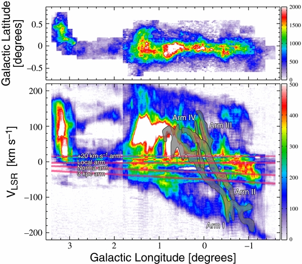
Figure 2. (a) Integrated intensity (∫TMBdV) map of CO J = 1–0 emission. The emission was integrated over velocities between VLSR = −200 km s−1 and +200 km s−1, and the map has been smoothed to 45'' resolution. (b) Longitude–velocity map of CO J = 1–0 emission integrated over the observed latitudes (∑TMB). The map has been smoothed to 45'' resolution and summed up to each +2 km s−1 bin. Magenta lines denote the l–V loci of spiral arms in the Galactic disk (+20 km s−1, local, Norma, and 3 kpc arms). Gray shaded areas indicate the molecular arms I–V identified in the 13CO data set (Sofue 1995).
Download figure:
Standard image High-resolution imageThe longitude–velocity behavior of CO J = 3–2 emission (Figure 1(b)) also resembles that of CO J = 1–0 (Figure 2(b)). Intense CO J = 3–2 emission from the main body of the CMZ appears as several curved chains of clouds in the l–V map, forming a large ridge of intense CO emission. These chains of clouds correspond to the molecular arms I–IV identified by Sofue (1995). The intense emission ridge is cut off at several velocities by the intervening spiral arms in the Galactic disk (3 kpc, 4.5 kpc, local, and +20 km s−1 arms in order of velocity). The positive-velocity component of the expanding molecular ring (EMR) can be traced as a gentle arc running from (l, VLSR) = (+ 14, +200 km s−1) to (− 08, +100 km s−1), while the negative-velocity counterpart of the EMR defines the negative velocity end of CO emission. The intensity discontinuities in the CO J = 3–2 l–V map at l = −13, −10, −028, +17, etc., are caused by the discontinuous variation in latitudinal coverage of the survey.
A prominent high-velocity feature appears at (l, VLSR) = (+ 125, +160 km s−1), which is the hyperenergetic shell CO 1.27+0.01 located in the center of the l = +13 complex (Oka et al. 2001a; Tanaka et al. 2007). Another prominent high-velocity feature, at (l, VLSR) = (+ 05, +130 km s−1), consists of a wing emission at b = 00 and a compact cloud at b ≃ +03. A compact feature at (l, b, VLSR) = (− 04, −025, −80 km s−1) is an HVCC, CO –0.41–0.23, which exhibits a high CO J = 3–2/CO J = 1–0 ratio (R3–2/1–0 ⩾ 1.5). In addition, we see a number of high-velocity features at the velocity ends of the intense emission ridge. Many of them correspond to HVCCs identified in the CO J = 1–0 data set (Nagai 2008). A faint high-velocity feature at (l, VLSR) = (− 01, −100 km s−1) is the negative-velocity component of the circumnuclear disk (CND; e.g., Oka et al. 2011a, and references therein).
3.2. Comparison with the CO J = 1–0 Line Intensity
3.2.1. Longitudinal and Latitudinal Distributions
Longitudinal distributions of the CO J = 3–2 (present work) and CO J = 1–0 line emissions (Oka et al. 1998b) are shown in Figure 3(a). There is no CO J = 3–2 data between l ≃ +18 and +28. Five prominent peaks at l ≃ −05, +01, +07, +13, and +31 correspond to the Sgr C, Sgr A, Sgr B, and l = +13 complexes, and Clump 2, respectively. These longitudinal distributions are naturally similar, showing high asymmetry with respect to the center, l = 0°. The l = +13 complex is the most prominent in these low-J CO lines, especially in the J = 1–0 line.
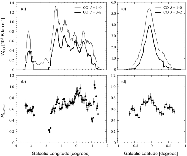
Figure 3. (a) Longitudinal distributions of CO J = 3–2 (thick line) and CO J = 1–0 (thin line) integrated intensities. (b) Longitudinal distribution of the ratio between the CO J = 3–2/CO J = 1–0 integrated intensities. (c) Latitudinal distributions of CO J = 3–2 (thick line) and CO J = 1–0 (thin line) integrated intensities. (d) Latitudinal distribution of the ratio between the CO J = 3–2/CO J = 1–0 integrated intensities. The integrated intensities are calculated by summing up the velocity-integrated intensities for positions where both J = 3–2 and J = 1–0 spectra have been obtained and averaged every 5 channels.
Download figure:
Standard image High-resolution imageLatitudinal distributions of the J = 3–2 and J = 1–0 line emissions are shown in Figure 3(c). The intensity distributions show roughly symmetrical profiles with respect to the midplane, b = −005. An abrupt change in the J = 3–2 intensity at b = +035 and −045 is due to the significant change in the longitudinal coverage of the data. A shoulder at b ≃ +03 is mainly attributed to the positive latitude flare-up of the l = +13 complex. A faint shoulder in the J = 3–2 profile at b ≃ −02 is due to the l = −04 region, where high R3–2/1–0 (⩾1.5) gas is abundant (Section 3.4.2).
3.2.2. CO J = 3–2/J = 1–0 Intensity Ratio
We often employ ratios between line intensities in the diagnoses of physical conditions or chemical compositions of interstellar gas. For instance, the CO J = 3–2/CO J = 1–0 intensity ratio (R3–2/1–0) is known to be a good indicator of the excitation of molecular gas, since the ratio is sensitive to the temperature and density of molecular gas (e.g., Oka et al. 2007). Figures 3(b) and (d) show the longitudinal and latitudinal distributions of the ratio of the CO J = 3–2 and CO J = 1–0 integrated intensities (≡ W3–2/W1–0). The integrated intensities, W3–2 and W1–0, are calculated by summing up the velocity-integrated intensities for positions where both J = 3–2 and J = 1–0 spectra have been obtained. The CO J = 1–0 data are from the NRO 45 m survey (Oka et al. 1998b).
Three cloud complexes, the Sgr A, Sgr B, and l = +13 complexes, are apparent in the longitudinal distribution of the ratio (Figure 3(b)). The highest ratio (≃ 1.05) in the longitudinal distribution is found at l ≃ −12, where a clump with very high R3–2/1–0 (∼2) resides (Section 3.4.2). The second highest ratio (≃ 0.95) is found at l ≃ −0.3, where a high R3–2/1–0 HVCC, CO –0.30–0.07 has been identified (Nagai 2008). The ratios at several longitudes are affected by such local high R3–2/1–0 regions, since the latitudinal coverages are not sufficient at these longitudes. A gap between the Sgr A and Sgr C complexes, which is apparent in the intensity distributions, is less prominent in the ratio distribution. Note that the Sgr C complex includes the l = −04 region, where several HVCCs and clumps with very high R3–2/1–0 ∼ 2 are included (Section 3.4.2). In the latitudinal distribution, the ratio gradually decreases with increasing distance from the midplane (Figure 3(d)). A small hump at b ≃ −02 corresponds to the faint shoulder in the J = 3–2 profile (Figure 3(c)), which is due to the l = −04 region. Except for small-scale deviations, the overall behavior of the CO J = 3–2/CO J = 1–0 integrated intensity ratio is similar to that of the CO J = 2–1/CO J = 1–0 ratio (Oka et al. 1998a).
Figure 4 shows the frequency distribution of the CO J = 3–2/J = 1–0 main-beam temperature ratio [TMB(CO J = 3 − −2)/TMB(CO J = 1 − −0)] weighted by the CO J = 1–0 intensity. Data with 1σ detections in both lines were used for the analysis. The contributions of four foreground spiral arms in the Galactic disk are denoted by gray bars. The spiral arms were defined by straight lines in the l–V plane, having velocity widths of 2 km s−1 (+20 km s−1 arm) or 4 km s−1 (local, 4.5 kpc, 3 kpc arms). Their l–V loci are presented in Figure 2(b). The R3–2/1–0 distribution has a prominent peak at 0.7, which is smaller than the peak observed in the preliminary results (Oka et al. 2007). This discrepancy is due to the increase in data points at a higher latitude, where R3–2/1–0 is lower. The R3–2/1–0 distribution also has a shoulder at ∼0.5, which is mostly attributable to the spiral arms. The R3–2/1–0 distribution of the spiral arms has a peak at 0.4 and a broad wing in the high-ratio side. The bulk of molecular gas in the CMZ has a higher R3–2/1–0 than that in the spiral arms in the Galactic disk, suggesting higher density and/or higher temperature in the CMZ. The total CO J = 3–2/J = 1–0 luminosity ratio was 0.71.
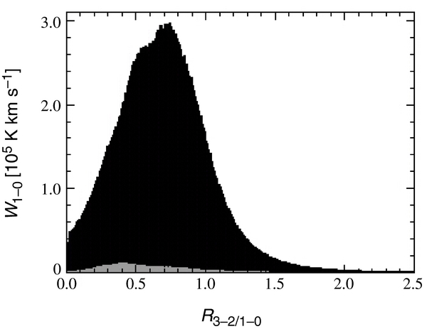
Figure 4. Frequency distribution of the CO J = 3–2/CO J = 1–0 intensity ratio (R3–2/1–0) weighted by the CO J = 1–0 intensity. The gray area shows the contributions of four spiral arms in the Galactic disk.
Download figure:
Standard image High-resolution image3.2.3. Intensity Correlation
Intensity correlations between different molecular lines are occasionally useful to infer the bulk physical conditions of molecular gas. Figure 5 presents a scatter plot of CO J = 1–0 and CO J = 3–2 intensities. Each data set has been smoothed to 60'' resolution and summed up to each +2 km s−1 bin. The CO J = 1–0 versus CO J = 3–2 scatter plot shows a tight positive correlation as a matter of course. Data points concentrate around the TMB(CO J = 1 − −0) = TMB(CO J = 3 − −2) line. A linear least-squares regression gives TMB(CO J = 3 − −2) = (− 0.222 ± 0.014) + (0.816 ± 0.004) × TMB(CO J = 1 − −0). The negative intersection with the TMB(CO J = 3 − −2) axis is due to an increase in the slope with increasing intensities. In other words, data points with higher intensities tend to have higher R3–2/1–0.
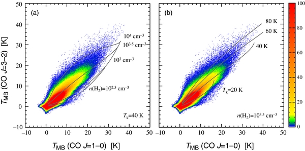
Figure 5. (a) A scatter plot of CO J = 1–0 and CO J = 3–2 main-beam temperatures. The color bar shows the number of data points included in each pixel. The pixel size is 0.1 K × 0.1 K. Gray curves show the CO J = 1–0 vs. CO J = 3–2 intensities calculated for various densities and Tk = 40 K. (b) Same as (a), with curves of CO J = 1–0 vs. CO J = 3–2 intensities for various temperatures and n(H2) = 103.5 cm−3.
Download figure:
Standard image High-resolution imageThe gray curves in Figure 5 show the results of LVG model calculations (Goldreich & Kwan 1974). Through simple visual inspection, we learn that a single component model with a particular set of density and temperature is inapplicable. A naive least-square fit gives n(H2) = 104.0 cm−3 and Tk = 18 K. This is significantly affected by data at lower intensities (TMB < 10 K), where the data density is very high (red area in Figure 5). This set of parameters might be inaccurate, since a higher temperature (Tk ≳ 30 K) has been suggested by a number of previous studies (e.g., Morris et al. 1983; Nagai et al. 2007).
The bulk behavior of the scatter plot roughly follows the model curve with n(H2) = 103.5 cm−3 and Tk = 40 K, while the small slope at TMB(CO J = 1 − −0) < 10 K can be reproduced by model curves with lower density [n(H2) ≲ 103.5 cm−3] or lower temperature Tk ≲ 40 K. The data points at higher intensities (TMB > 20 K) are well above the n(H2) = 103.5 cm−3 and Tk = 40 K curve, indicating higher temperature and higher density for these points.
3.3. Data Presentation
The full data set of CO J = 3–2 emission is presented in the forms of velocity channel maps and longitude–velocity (l–V) maps with the corresponding maps of the CO J = 3–2/CO J = 1–0 intensity ratio. The line intensity maps are in units of main-beam temperature (TMB ≡ T*A/ηMB).
3.3.1. Velocity Channel Maps
Figure 6 shows CO J = 3–2 velocity channel maps integrated over successive 10 km s−1 widths and the corresponding maps of the CO J = 3–2/CO J = 1–0 integrated intensity ratio. The maps were created from the quantities at the original observational grid and by smoothing with a 45'' (FWHM) Gaussian weighting function. The intensity ratios were calculated for data pixels where both CO J = 3–2 and CO J = 1–0 lines are detected with 3σ confidence.
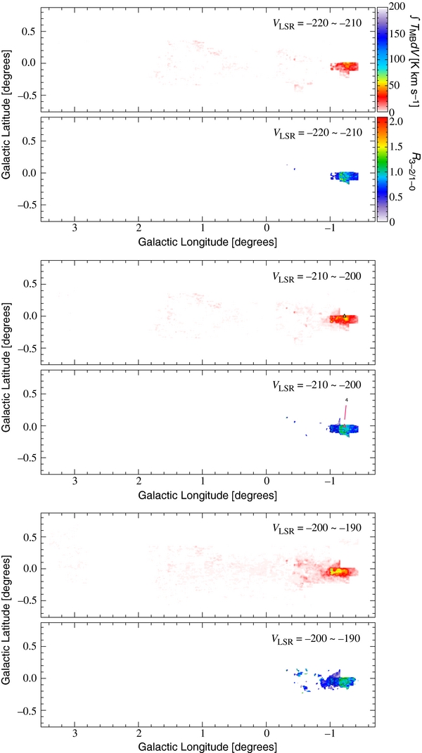
Figure 6.
Velocity channel maps of CO J = 3–2 line emission integrated over successive 10 km s−1 widths (upper panels) and the corresponding maps of CO J = 3–2/CO J = 1–0 integrated intensity ratio (lower panels). Contours are set at intervals of 30 K km s−1. Open circles indicate spots located at cloud edges, open triangles indicate those in the velocity end, saltire crosses indicate those appearing as high-velocity wings, Greek crosses indicate those associated with HVCCs or HVCC-like features, open squares indicate those in shells or emission cavities, and filled circles indicate those associated with small clumps. Numbers are those in Table 1. (An extended, color version of this figure is available in the online journal.)
Download figure:
Standard image High-resolution image3.3.2. Longitude–Velocity Maps
Figure 7 shows CO J = 3–2 l–V maps and the corresponding maps of the CO J = 3–2/CO J = 1–0 main-beam temperature ratio. The l–V maps cover the velocity range VLSR = −220 km s−1 to +220 km s−1 and are presented at a latitude interval of 2' (=0033), starting with b = −40' and ending at b = +38'. The l–V maps were created by interpolating the quantities onto each latitudinal cut. The data were summed over each 2.0 km s−1 velocity bin and smoothed with a 45'' (FWHM) Gaussian weighting function.

Figure 7.
Longitude–velocity maps (l–V maps) of CO J = 3–2 line emission (upper panels) and the corresponding maps of the CO J = 3–2/CO J = 1–0 main-beam temperature ratio (lower panels). Contours are set at intervals of 5 K. Symbols and numbers are the same as those in Figure 6. HVCCs apparent in the CO J = 3–2 data are indicated by ellipses. (An extended, color version of this figure is available in the online journal.)
Download figure:
Standard image High-resolution image3.4. Features with High CO J = 3–2/CO J = 1–0 Intensity Ratio
3.4.1. Extraction of High Ratio Gas
A number of high R3–2/1–0 regions can be seen in Figures 6 and 7. High R3–2/1–0, well exceeding unity, has been found in UV-irradiated cloud surfaces near massive stars (e.g., White et al. 1999) and shocked molecular gas adjacent to supernova remnants (e.g., Arikawa et al. 1999). The high R3–2/1–0 regions detected in the Galactic center might indicate such UV-irradiated gas or shocked gas. In order to illustrate the spatial and longitude–velocity distributions of high R3–2/1–0 gas, we created maps of CO J = 3–2 emission by integrating the data with R3–2/1–0 ⩾ 1.5 (Figure 8). Henceforth in this paper, "high" ratio implies R3–2/1–0 ⩾ 1.5. Data with 1σ detections in both lines were used for the analysis. Data severely contaminated by the foreground disk gas, (− 55 + 10 l) km s−1 ⩽VLSR ⩽ +15 km s−1, where l is the Galactic longitude in degrees, were excluded from the velocity integration in creating the map shown in Figure 8(a). One-zone LVG calculations indicate that R3–2/1–0 ⩾ 1.5 corresponds to n(H2) ⩾ 103.6 cm−3 and Tk ⩾ 48 K when NCO/dV = 1017 cm−2 (km s−1)−1 (Oka et al. 2007). Note that subthermally excited gas in the foreground can increase R3–2/1–0 by selectively absorbing J = 1–0 photons (Oka et al. 2007). Narrow-velocity-width high R3–2/1–0 features in the velocity range of −60 km s−1 ⩽VLSR ⩽ +15 km s−1 might be due to such selective absorption by a subthermally excited gas in the Galactic disk. The high R3–2/1–0 region at l ∼ 09 seen in the preliminary results (Oka et al. 2007) disappeared with improved data quality. This could be mainly due to the baseline ripple of spectra presented in the previous paper.

Figure 8. (a) A map of CO J = 3–2 emission (∫TMB dV) integrated over velocities VLSR between −200 km s−1 and +200 km s−1 for data with R3–2/1–0 ⩾ 1.5. Data severely contaminated by the foreground disk gas, (− 55 + 10 l) km s−1 ⩽VLSR ⩽ +15 km s−1, have been excluded. (b) Longitude–velocity map of CO J = 3–2 emission integrated over the observed latitudes (∑TMB) for data with R3–2/1–0 ⩾ 1.5.
Download figure:
Standard image High-resolution image3.4.2. High Ratio Clumps
Sgr A region. This is a high R3–2/1–0 clump with a size of 6' × 4' at Sgr A and a small redshifted clump in its Galactic northwest. The small redshifted clump is a well-known HVCC, CO 0.02–0.02 (Oka et al. 1999). The Sgr A clump splits up several components in the l–V plane. It contains the CND (Oka et al. 2011b), several clumps that might be adjacent to the CND, and the positive velocity end of the bridge that connects M–0.02–0.07 (+50 km s−1 cloud) and M–0.13–0.08 (+20 km s−1 cloud). Details of this high R3–2/1–0 clump have been discussed in the preceding papers (Oka et al. 2007; Oka et al. 2011b).
l = +13 region. This high R3–2/1–0 clump is located at the root of the l = +13 complex, which elongates to a positive Galactic latitude ∼05. It stands out in the l–V map owing to its extremely large velocity width. This clump consists of two expanding shells (Oka et al. 2001a). High-resolution HCN J = 1–0 maps have indicated that at least nine expanding shells are included in this region and that several isolated SiO clumps are associated with the expanding shells (Tanaka et al. 2007). These results suggest that the high R3–2/1–0 clump in the l = +13 region might have been generated by a series of supernova explosions. The enormous kinetic energy (2 × 1052 erg) and the short expansion time (6 × 10⁴ years) indicate that a massive stellar cluster is embedded in this region and that the region could be at an early stage of superbubble formation (as a proto-superbubble; Tanaka et al. 2007). The details of this anomalous region have been discussed in the preceding papers (Oka et al. 2001a; Tanaka et al. 2007).
l = −04 region. This is a large (∼03 × 03), arc-shaped high R3–2/1–0 clump with complex kinematics. It includes a high R3–2/1–0 HVCC, CO –0.41–0.21 (Nagai 2008). This high R3–2/1–0 region might be distinct from the Sgr C cloud. Molecular gas in the l = −04 region is probably in Arm I, while the Sgr C H ii region belongs to Arm II (Sofue 1995). Unfortunately, this high R3–2/1–0 clump is separated by the absorption features of the foreground arms. The arc-shaped, off-plane morphology and the association of a high R3–2/1–0 HVCC suggest that the high R3–2/1–0 clump at l ≃ −04 might have been generated by a series of supernova explosions and that it may be another candidate for proto-superbubble. Details of this region will be discussed in a forthcoming paper (K. Tanaka et al. 2012, in preparation).
l = −12 region. This well-defined high R3–2/1–0 clump appears at (l, b) ≃ (− 122, −012) in the vicinity of Sgr E, showing the clear kinematics of an expanding shell. A part of this shell has been identified as a high R3–2/1–0 HVCC, CO –1.22–0.14 (Nagai 2008). The kinetic energy amounts to 5 × 1049 erg, and the expansion time is about 9 × 10⁴ years. No infrared or radio counterpart was detected in the shell. Details of this region will be discussed elsewhere.
3.4.3. High Ratio Spots
In addition to the high R3–2/1–0 clumps described in the previous section, we see a number of small spots of high R3–2/1–0 gas. We identified these high R3–2/1–0 spots in an automated manner with a TMB ⩾ 1.0 K threshold in the R3–2/1–0 ⩾ 1.5 clipped CO J = 3–2 data cube. Before the identification procedure, data severely contaminated by the foreground disk gas, which is defined by (− 55 + 10 l) km s−1 ⩽VLSR ⩽ +15 km s−1, were excluded. Very small clumps with less than 10 pixels were eliminated from the list. Table 1 lists 176 high R3–2/1–0 spots and clumps to serve as a record for further research. We categorized these spots into six groups based on the situation in which they are located.
Table 1. High R3–2/1–0 Spots and Clumps in the Galactic Center Region
| Number | l | b | VLSR | Δl | Δb | ΔV | Comments |
|---|---|---|---|---|---|---|---|
| (deg) | (deg) | (km s−1) | (deg) | (deg) | (km s−1) | ||
| 1 | −1.40 | −0.11 | −139 | 0.04 | 0.03 | 28 | HVCC, CO –1.41–0.08 |
| 2 | −1.29 | −0.19 | −73 | 0.01 | 0.03 | 14 | Velocity end |
| 3 | −1.29 | −0.13 | −77 | 0.01 | 0.05 | 28 | Velocity end? |
| 4 | −1.22 | 0.01 | −200 | 0.07 | 0.02 | 14 | Velocity end? |
| 5 | −1.21 | −0.12 | −125 | 0.11 | 0.09 | 86 | Includes HVCC, CO –1.21–0.12, |
| in the l = −12 region | |||||||
| 6 | −1.20 | 0.01 | −186 | 0.03 | 0.01 | 8 | Velocity end |
| 7 | −1.10 | −0.23 | −72 | 0.05 | 0.02 | 12 | Velocity end |
| 8 | −0.98 | 0.08 | −83 | 0.04 | 0.04 | 14 | Velocity end of a small cloud |
| 9 | −0.94 | 0.02 | −81 | 0.07 | 0.08 | 18 | Velocity end of a small cloud |
| 10 | −0.90 | −0.22 | −105 | 0.08 | 0.03 | 28 | Edge of map |
| 11 | −0.85 | 0.10 | −105 | 0.04 | 0.03 | 10 | HVCC-like |
| 12 | −0.81 | 0.17 | −115 | 0.05 | 0.03 | 24 | HVCC, CO –0.79+0.16 |
| 13 | −0.80 | 0.10 | −65 | 0.04 | 0.04 | 10 | HVCC, CO –0.80+0.11 |
| 14 | −0.77 | 0.19 | 31 | 0.02 | 0.04 | 10 | HVCC, CO –0.79+0.18 |
| 15 | −0.76 | −0.23 | −97 | 0.05 | 0.01 | 18 | Edge of map |
| 16 | −0.76 | 0.19 | −98 | 0.03 | 0.03 | 10 | HVCC, CO –0.79+0.16 |
| 17 | −0.66 | −0.29 | −66 | 0.03 | 0.03 | 12 | HVCC-like |
| 18 | −0.64 | −0.29 | 21 | 0.11 | 0.18 | 22 | High ratio clump |
| 19 | −0.63 | 0.04 | −104 | 0.03 | 0.02 | 14 | HVCC, CO –0.63–0.07 |
| 20 | −0.62 | −0.28 | −79 | 0.03 | 0.03 | 14 | Cloud edge |
| 21 | −0.62 | −0.03 | −102 | 0.10 | 0.04 | 4 | High ratio clump |
| including a velocity end | |||||||
| 22 | −0.61 | −0.07 | −139 | 0.04 | 0.02 | 10 | Velocity end |
| 23 | −0.60 | 0.35 | 120 | 0.02 | 0.02 | 8 | Velocity end of a small cloud |
| 24 | −0.60 | −0.13 | 42 | 0.04 | 0.03 | 4 | Expanding shell |
| 25 | −0.60 | −0.02 | −94 | 0.05 | 0.02 | 8 | Cloud edge, velocity end |
| 26 | −0.59 | −0.32 | −153 | 0.06 | 0.02 | 24 | HVCC-like |
| 27 | −0.58 | −0.14 | 76 | 0.06 | 0.04 | 14 | High-velocity wing of a small clump, |
| cloud edge of a small cloud | |||||||
| 28 | −0.56 | −0.23 | −162 | 0.04 | 0.02 | 14 | Cloud edge? |
| 29 | −0.56 | −0.23 | −135 | 0.04 | 0.03 | 6 | Velocity end |
| 30 | −0.55 | 0.11 | 37 | 0.04 | 0.04 | 20 | Foreground arm?, bad quality |
| 31 | −0.55 | 0.12 | −96 | 0.04 | 0.03 | 8 | HVCC, CO –0.51+0.12 |
| 32 | −0.55 | 0.00 | −73 | 0.09 | 0.03 | 12 | Velocity end |
| 33 | −0.54 | −0.07 | −71 | 0.04 | 0.03 | 2 | Velocity end |
| 34 | −0.54 | 0.20 | −152 | 0.04 | 0.04 | 24 | Cloud edge |
| 35 | −0.54 | −0.29 | −137 | 0.07 | 0.08 | 38 | Cloud edge |
| 36 | −0.53 | −0.10 | −61 | 0.04 | 0.04 | 2 | Cloud edge |
| 37 | −0.51 | 0.09 | −136 | 0.06 | 0.04 | 4 | HVCC, CO –0.51+0.12 |
| 38 | −0.50 | −0.04 | −84 | 0.04 | 0.03 | 8 | Velocity end |
| 39 | −0.49 | 0.01 | −81 | 0.07 | 0.04 | 4 | Velocity end |
| 40 | −0.48 | −0.01 | 27 | 0.02 | 0.06 | 8 | Cloud edge |
| 41 | −0.48 | −0.25 | −152 | 0.04 | 0.03 | 14 | Velocity end |
| 42 | −0.47 | −0.25 | −141 | 0.08 | 0.03 | 6 | Velocity end |
| 43 | −0.47 | −0.21 | −82 | 0.37 | 0.33 | 80 | l = −04 region including HVCC, |
| CO –0.41–0.23, and HVCC, CO –0.54–0.17 | |||||||
| 44 | −0.45 | −0.01 | −74 | 0.04 | 0.04 | 10 | Velocity end |
| 45 | −0.37 | −0.02 | −64 | 0.03 | 0.02 | 10 | Cloud edge |
| 46 | −0.35 | −0.12 | −63 | 0.06 | 0.06 | 14 | HVCC-like |
| 47 | −0.34 | 0.21 | −61 | 0.03 | 0.03 | 8 | Velocity end of a small cloud |
| 48 | −0.32 | −0.07 | 88 | 0.03 | 0.03 | 6 | HVCC, CO –0.30–0.07 |
| 49 | −0.32 | −0.06 | 61 | 0.03 | 0.04 | 24 | HVCC, CO –0.30–0.07 |
| 50 | −0.31 | −0.06 | 98 | 0.09 | 0.06 | 14 | HVCC, CO –0.30–0.07 |
| 51 | −0.30 | 0.10 | −62 | 0.03 | 0.04 | 10 | Cloud edge? |
| 52 | −0.30 | 0.05 | 48 | 0.07 | 0.04 | 18 | Cloud edge |
| 53 | −0.27 | −0.22 | 38 | 0.05 | 0.04 | 12 | Cloud edge? |
| 54 | −0.27 | −0.03 | 37 | 0.16 | 0.12 | 48 | Includes an HVCC-like feature |
| 55 | −0.27 | 0.01 | −76 | 0.15 | 0.16 | 62 | Includes a velocity end |
| 56 | −0.25 | −0.18 | 25 | 0.04 | 0.03 | 10 | Cloud edge? |
| 57 | −0.24 | 0.05 | 22 | 0.04 | 0.08 | 8 | Velocity end |
| 58 | −0.23 | −0.19 | 18 | 0.09 | 0.05 | 6 | Cloud edge |
| 59 | −0.22 | −0.19 | 40 | 0.02 | 0.02 | 10 | Velocity end of a small cloud |
| 60 | −0.18 | −0.12 | 82 | 0.09 | 0.04 | 22 | Cloud edge? |
| 61 | −0.13 | 0.01 | 47 | 0.06 | 0.07 | 16 | Cloud edge? |
| 62 | −0.13 | 0.08 | 39 | 0.02 | 0.03 | 12 | HVCC, CO –0.13+0.03 |
| 63 | −0.10 | 0.10 | 85 | 0.06 | 0.03 | 18 | Cloud edge |
| 64 | −0.09 | −0.04 | 17 | 0.06 | 0.04 | 2 | Sgr A |
| 65 | −0.09 | 0.00 | 18 | 0.04 | 0.03 | 6 | Cloud edge |
| 66 | −0.08 | 0.18 | 79 | 0.02 | 0.03 | 12 | HVCC-like |
| 67 | −0.06 | −0.04 | −77 | 0.15 | 0.16 | 68 | Includes HVCC, CO –0.02–0.02 |
| associated with Sgr A region | |||||||
| 68 | −0.06 | −0.05 | 62 | 0.15 | 0.12 | 120 | Includes HVCC, CO –0.04–0.08, |
| associated with Sgr A region | |||||||
| 69 | −0.03 | −0.08 | 22 | 0.09 | 0.06 | 16 | HVCC, CO –0.00–0.11, |
| associated with Sgr A region | |||||||
| 70 | 0.00 | 0.04 | 48 | 0.06 | 0.04 | 14 | Cloud edge |
| 71 | 0.01 | 0.01 | 20 | 0.05 | 0.08 | 10 | Cloud edge |
| 72 | 0.05 | −0.02 | 76 | 0.01 | 0.03 | 18 | Root of a high-velocity wing |
| 73 | 0.05 | −0.09 | 25 | 0.04 | 0.06 | 20 | Cloud edge? |
| 74 | 0.06 | 0.18 | 85 | 0.04 | 0.04 | 14 | Velocity end |
| 75 | 0.07 | −0.06 | −58 | 0.04 | 0.05 | 10 | Velocity end? |
| 76 | 0.09 | −0.07 | 29 | 0.03 | 0.04 | 10 | HVCC, CO 0.10–0.11 |
| 77 | 0.09 | −0.14 | 34 | 0.03 | 0.06 | 10 | HVCC, CO 0.10–0.11 |
| 78 | 0.09 | −0.02 | 80 | 0.03 | 0.03 | 12 | HVCC, CO 0.10–0.04 |
| 79 | 0.12 | −0.14 | 47 | 0.07 | 0.05 | 12 | Velocity end |
| 80 | 0.12 | −0.20 | 28 | 0.03 | 0.03 | 14 | HVCC, CO+0.10–0.24 |
| 81 | 0.13 | −0.02 | −92 | 0.04 | 0.06 | 6 | High-velocity wing |
| 82 | 0.14 | 0.06 | 17 | 0.03 | 0.06 | 4 | Velocity end? |
| 83 | 0.14 | −0.09 | 94 | 0.06 | 0.05 | 28 | HVCC, CO 0.18–0.10 |
| 84 | 0.16 | −0.17 | 48 | 0.05 | 0.03 | 18 | Cloud edge |
| 85 | 0.18 | −0.04 | 93 | 0.02 | 0.04 | 12 | Velocity end |
| 86 | 0.18 | −0.11 | 108 | 0.05 | 0.07 | 20 | HVCC, CO 0.18–0.10 |
| 87 | 0.19 | −0.16 | 76 | 0.02 | 0.03 | 8 | Cloud edge |
| 88 | 0.19 | 0.05 | 23 | 0.01 | 0.04 | 14 | Cloud edge |
| 89 | 0.20 | −0.06 | 19 | 0.02 | 0.03 | 8 | Cloud edge |
| 90 | 0.23 | −0.18 | 81 | 0.07 | 0.05 | 28 | Edge of the expanding cavity |
| 91 | 0.23 | 0.02 | 48 | 0.03 | 0.04 | 8 | HVCC, CO 0.25+0.02 |
| 92 | 0.23 | 0.05 | 38 | 0.02 | 0.03 | 12 | HVCC, CO 0.25+0.02 |
| 93 | 0.24 | −0.06 | 21 | 0.04 | 0.07 | 8 | Cloud edge |
| 94 | 0.25 | −0.07 | 47 | 0.04 | 0.07 | 18 | Inner rim of the expanding cavity |
| 95 | 0.26 | −0.14 | 50 | 0.08 | 0.05 | 30 | HVCC-like in the edge of expanding cavity |
| 96 | 0.29 | −0.17 | 21 | 0.12 | 0.11 | 20 | A clump in the 20 km s−1 arm |
| 97 | 0.30 | 0.02 | 38 | 0.05 | 0.09 | 20 | Velocity end |
| 98 | 0.30 | −0.08 | 24 | 0.03 | 0.03 | 4 | Cloud edge |
| 99 | 0.30 | −0.08 | 57 | 0.04 | 0.05 | 14 | HVCC-like in the edge of expanding cavity |
| 100 | 0.33 | −0.19 | −65 | 0.03 | 0.03 | 8 | HVCC-like |
| 101 | 0.36 | −0.01 | 95 | 0.04 | 0.03 | 12 | Cloud edge, velocity end |
| 102 | 0.36 | −0.30 | −89 | 0.02 | 0.03 | 6 | Cloud edge? |
| 103 | 0.36 | 0.00 | 56 | 0.02 | 0.03 | 8 | Cavity |
| 104 | 0.37 | −0.06 | 107 | 0.22 | 0.12 | 44 | Velocity end |
| 105 | 0.42 | 0.07 | 111 | 0.04 | 0.05 | 8 | Cloud edge |
| 106 | 0.43 | 0.01 | 54 | 0.04 | 0.05 | 8 | Cavity |
| 107 | 0.43 | 0.05 | 62 | 0.04 | 0.04 | 22 | Cloud edge?, velocity end? |
| 108 | 0.44 | 0.05 | 96 | 0.04 | 0.04 | 10 | HVCC-like |
| 109 | 0.48 | −0.06 | 116 | 0.04 | 0.05 | 12 | Velocity end |
| 110 | 0.51 | 0.01 | 60 | 0.08 | 0.09 | 16 | Cavity |
| 111 | 0.53 | −0.05 | 115 | 0.04 | 0.04 | 14 | High-velocity wing |
| 112 | 0.54 | 0.05 | 75 | 0.04 | 0.06 | 8 | Cloud edge |
| 113 | 0.55 | 0.06 | 57 | 0.02 | 0.02 | 12 | HVCC-like |
| 114 | 0.58 | −0.21 | 30 | 0.04 | 0.05 | 16 | Cloud edge |
| 115 | 0.59 | −0.03 | 118 | 0.04 | 0.02 | 8 | Velocity end |
| 116 | 0.59 | −0.28 | −84 | 0.03 | 0.02 | 8 | HVCC-like |
| 117 | 0.59 | −0.21 | 65 | 0.05 | 0.04 | 10 | Cloud edge |
| 118 | 0.63 | −0.02 | 127 | 0.06 | 0.05 | 20 | High-velocity wing |
| 119 | 0.66 | −0.10 | 17 | 0.04 | 0.07 | 2 | Clump |
| 120 | 0.68 | −0.07 | 119 | 0.03 | 0.03 | 22 | High-velocity wing |
| 121 | 0.72 | −0.06 | 17 | 0.04 | 0.04 | 4 | In a cloud |
| 122 | 0.73 | 0.20 | 21 | 0.03 | 0.02 | 12 | HVCC, CO 0.77+0.15, bad quality |
| 123 | 0.79 | 0.17 | 41 | 0.10 | 0.09 | 46 | Includes HVCC, CO 0.77+0.15, bad quality |
| 124 | 0.80 | 0.18 | 85 | 0.05 | 0.05 | 10 | HVCC, CO 0.77+0.15, bad quality |
| 125 | 0.81 | 0.17 | 108 | 0.05 | 0.07 | 16 | HVCC, CO 0.77+0.15, bad quality |
| 126 | 0.82 | 0.13 | 76 | 0.05 | 0.03 | 8 | HVCC, CO 0.77+0.15, bad quality |
| 127 | 0.83 | 0.03 | −74 | 0.05 | 0.04 | 12 | HVCC, CO 0.83+0.03, |
| associated with SNR G0.9+0.1? | |||||||
| 128 | 0.84 | 0.03 | −110 | 0.03 | 0.04 | 14 | HVCC, CO 0.84+0.03, |
| associated with SNR G0.9+0.1? | |||||||
| 129 | 0.84 | 0.02 | −99 | 0.06 | 0.04 | 8 | HVCC, CO 0.84+0.03, |
| associated with SNR G0.9+0.1? | |||||||
| 130 | 0.84 | −0.12 | 81 | 0.03 | 0.04 | 12 | In a cloud |
| 131 | 0.85 | −0.18 | 77 | 0.01 | 0.03 | 16 | HVCC, CO 0.84–0.18 |
| 132 | 0.86 | 0.00 | −89 | 0.09 | 0.05 | 14 | HVCC, CO 0.84+0.03, |
| associated with SNR G0.9+0.1? | |||||||
| 133 | 0.88 | 0.12 | −55 | 0.03 | 0.04 | 6 | HVCC-like |
| 134 | 0.88 | −0.07 | 45 | 0.02 | 0.02 | 22 | HVCC, CO 0.88–0.07 |
| 135 | 0.92 | 0.16 | −65 | 0.03 | 0.04 | 6 | HVCC-like |
| 136 | 0.93 | 0.14 | 77 | 0.15 | 0.09 | 52 | Includes a velocity end, bad quality |
| 137 | 0.95 | 0.06 | −67 | 0.18 | 0.17 | 36 | High ratio clump |
| 138 | 0.98 | −0.13 | 36 | 0.05 | 0.02 | 14 | High-velocity wing, cavity |
| 139 | 0.99 | −0.04 | 52 | 0.09 | 0.06 | 18 | Velocity end, cavity? |
| 140 | 1.03 | −0.12 | 61 | 0.02 | 0.05 | 6 | Cavity |
| 141 | 1.13 | 0.10 | 50 | 0.03 | 0.04 | 20 | HVCC, CO 1.17+0.08 |
| 142 | 1.13 | −0.09 | 41 | 0.03 | 0.04 | 16 | Velocity end |
| 143 | 1.14 | −0.27 | 44 | 0.04 | 0.03 | 8 | Cloud edge?, velocity end? |
| 144 | 1.15 | 0.12 | 23 | 0.01 | 0.03 | 12 | HVCC, CO 1.16+0.24 |
| 145 | 1.16 | −0.28 | 61 | 0.05 | 0.07 | 10 | Cloud edge |
| 146 | 1.22 | 0.06 | 129 | 0.16 | 0.26 | 92 | Includes HVCC, CO 1.27+0.06, |
| associated with l = +13 region | |||||||
| 147 | 1.23 | −0.20 | 67 | 0.04 | 0.02 | 8 | HVCC, CO 1.26–0.19 |
| 148 | 1.26 | −0.28 | −79 | 0.04 | 0.07 | 6 | Velocity end |
| 149 | 1.29 | −0.21 | 62 | 0.07 | 0.04 | 14 | HVCC, CO 1.26–0.19 |
| 150 | 1.32 | −0.20 | −77 | 0.06 | 0.03 | 8 | Cloud edge |
| 151 | 1.32 | 0.35 | 76 | 0.02 | 0.01 | 14 | HVCC, CO 1.31+0.28 |
| 152 | 1.32 | −0.31 | 19 | 0.05 | 0.06 | 10 | Cloud edge? |
| 153 | 1.33 | −0.23 | 20 | 0.05 | 0.07 | 12 | In a small cloud |
| 154 | 1.33 | −0.26 | −54 | 0.04 | 0.12 | 18 | HVCC, CO 1.33–0.31 |
| 155 | 1.33 | −0.40 | 18 | 0.03 | 0.07 | 6 | HVCC-like |
| 156 | 1.33 | −0.35 | 90 | 0.03 | 0.02 | 8 | Cloud edge? |
| 157 | 1.34 | −0.30 | −80 | 0.05 | 0.09 | 10 | HVCC, CO 1.33–0.31 |
| 158 | 1.34 | 0.09 | 51 | 0.10 | 0.07 | 28 | Includes a velocity end |
| 159 | 1.35 | −0.50 | 62 | 0.02 | 0.04 | 16 | Velocity end? |
| 160 | 1.36 | 0.03 | 54 | 0.03 | 0.04 | 20 | High-velocity wing |
| 161 | 1.45 | 0.23 | 55 | 0.05 | 0.03 | 14 | Velocity end of a small cloud |
| 162 | 1.54 | −0.28 | −46 | 0.06 | 0.04 | 4 | Velocity end? |
| 163 | 1.55 | −0.66 | 38 | 0.01 | 0.03 | 12 | HVCC, CO 1.52–0.64 |
| 164 | 1.57 | −0.32 | −47 | 0.06 | 0.04 | 2 | Velocity end |
| 165 | 1.67 | −0.38 | −68 | 0.04 | 0.06 | 6 | HVCC-like |
| 166 | 1.68 | −0.36 | −48 | 0.05 | 0.12 | 22 | HVCC-like |
| 167 | 1.80 | −0.14 | 28 | 0.07 | 0.09 | 14 | Velocity end of a small clump? |
| 168 | 1.82 | −0.12 | 50 | 0.06 | 0.06 | 26 | Velocity end of a small clump? |
| 169 | 2.84 | 0.07 | 61 | 0.04 | 0.07 | 28 | HVCC-like, Clump2 |
| 170 | 2.85 | 0.06 | 109 | 0.01 | 0.03 | 24 | HVCC, CO 2.89+0.07, Clump2 |
| 171 | 3.03 | −0.07 | 28 | 0.05 | 0.04 | 12 | HVCC, CO 2.98–0.11, Clump2 |
| 172 | 3.16 | 0.26 | 22 | 0.03 | 0.02 | 12 | HVCC, CO 3.17+0.30, Clump2 |
| 173 | 3.23 | 0.52 | 18 | 0.09 | 0.08 | 6 | Cloud edge, Clump2 |
| 174 | 3.36 | 0.40 | 45 | 0.05 | 0.03 | 20 | HVCC-like, Clump2 |
| 175 | 3.37 | 0.40 | 72 | 0.05 | 0.03 | 16 | HVCC-like, Clump2 |
| 176 | 3.39 | 0.34 | 125 | 0.02 | 0.01 | 20 | HVCC-like, Clump2 |
Cloud edge. The spot is located at the spatial edge of a cloud.
Velocity end. The spot is located at the velocity end of a cloud.
HVCC(-like). The spot is associated with or corresponds to an HVCC listed in Nagai (2008) or an HVCC-like feature that seems to satisfy the definition of HVCC but is not listed in Nagai (2008).
High-velocity wing. The spot corresponds to a high-velocity wing emission feature.
Shell/emission cavity. The spot is associated with a shell-like structure or an emission cavity.
Clump. The spot corresponds to a small-velocity-width clump.
However, this categorization is slightly redundant since some high R3–2/1–0 spots show profiles of two categories. Most of the high R3–2/1–0 spots prefer the spatial edge or velocity end of clouds. Forty-eight high R3–2/1–0 spots are associated with the previously identified HVCCs (Nagai 2008), and 21 spots are associated with HVCC-like features in the CO J = 3–2 data. Forty-six are found in the velocity end of clouds and eight are categorized as high-velocity wings. Forty-two high R3–2/1–0 spots are found in the spatial edges of clouds, and 10 are in shells or emission cavities. Two small clumps with small velocity widths show a very high R3–2/1–0 ratio, but an LSR velocity around +20 km s−1 indicates that they might be in the foreground spiral arm and their high ratios could be an effect of absorption (Oka et al. 2007).
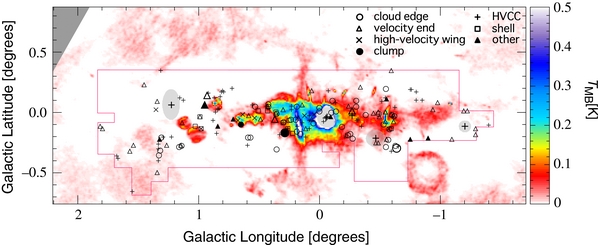
Figure 9 shows the spatial distribution of high R3–2/1–0 spots and clumps superposed on the VLA 90 cm image (LaRosa et al. 2000). Since the radio continuum data do not cover Clump 2, we present high R3–2/1–0 spots and clumps in the longitudinal range between −14 and +18. A number of R3–2/1–0 spots within |l| ⩽ 07 seem to be associated with intense radio continuum sources such as Sgr A, Sgr B, Sgr C, the vertical filaments of Radio Arc, and SNR G0.33+0.04 (Kassim & Frail 1996). A group of high R3–2/1–0 spots is associated with a composite SNR G0.9+0.1, which is bright in TeV gamma-rays (Aharonian et al. 2005). Two (or three) high R3–2/1–0 spots overlap with the thread in Sgr C, and one spot is adjacent to the thread at (l, b) ≃ (+ 01, +015). These high R3–2/1–0 spots could be regions of shocked molecular gas generated by the supernova/molecular cloud interaction. Such an association has already been found at the intersection between the nonthermal filament "Snake" and the SNR G359.1–0.5 (Yusef-Zadeh et al. 1995; Lazendic et al. 2002). These facts suggest that the supernova/molecular cloud interaction plays an important role in accelerating electrons and forming nonthermal threads and filaments, which are unique and abundant in the CMZ.
Figure 9. Spatial distribution of high ratio (R3–2/1–0 ⩾ 1.5) spots superposed on the VLA 90 cm image (LaRosa et al. 2000). Gray shaded areas show the high ratio clumps described in Section 3.4.2. The red line encloses the area of CO J = 3–2 data coverage. The open circles indicate spots located at cloud edges, open triangles indicate those in the velocity end of clouds, saltire crosses indicate those appear as high-velocity wings, Greek crosses indicate those associated with HVCCs or HVCC-like features, open squares indicate those in shells or emission cavities, and filled circles indicate those associated with small clumps.
Download figure:
Standard image High-resolution image
On the other hand, we also see a number of high R3–2/1–0 spots in the region without intense radio continuum emission. Although the origin of these spots is unknown, it could be relevant to interstellar shock, because many of them are associated with HVCCs or are found in the velocity end of clouds. Determining for the exciting sources of these high R3–2/1–0 spots without a radio continuum counterpart may be an important task to be carried out in the near future.
3.4.4. Interpretation of the Distribution of High Ratio Gas
The objective of this CO J = 3–2 survey is to investigate the origin of interstellar shock in the CMZ. In scenarios of large-scale shocks, extended distribution of shocked gas is expected along the Galactic longitude (e.g., Athanassoula 1992); however, the results of our analyses of R3–2/1–0 clearly differ from this expectation. We found several high R3–2/1–0 clumps and high R3–2/1–0 spots, most of which might be regions of shocked molecular gas excited by local explosive events. The observed distribution of high R3–2/1–0 gas supports the scenario that small-scale shocks by supernova explosions and/or Wolf–Rayet stellar winds dominate gas heating and turbulent activation in the CMZ. Indeed, the energy deposition rate provided by HVCCs is sufficient to maintain the turbulent motion and high temperature of molecular gas in the CMZ (Tanaka et al. 2009; Oka et al. 2011b).
4. SUMMARY
We have performed large-scale CO J = 3–2 mapping observations of the Galactic center region with the ASTE 10 m telescope. This paper presents the full data set of CO J = 3–2 emission in forms of velocity channel maps and longitude–velocity maps with the corresponding maps of R3–2/1–0. Our mapping area covers almost the full extent of the molecular gas concentration in the Galactic center, including the CMZ and Clump 2. The principal results of this survey are summarized as follows.
- 1.The spatial and longitude–velocity distributions of CO J = 3–2 emission show similar behavior to those of CO J = 1–0 emission.
- 2.Molecular gas in the Galactic center shows higher R3–2/1–0 (∼0.7) than gas in the spiral arms in the Galactic disk (∼0.4). The CO J = 3–2/J = 1–0 luminosity ratio is 0.71.
- 3.Typical physical conditions of molecular gas are n(H2) = 103.5 cm−3 and Tk = 40 K, although they include large uncertainties.
- 4.Four high R3–2/1–0 clumps are identified in the Sgr A, l = +13, l = −04, and l = −12 regions. These high R3–2/1–0 clumps have extremely large velocity widths, including HVCCs.
- 5.A number of small spots of high ratio gas with large velocity widths are also identified. Many of them have large velocity widths, suggesting that they are spots of hot molecular gas shocked by unidentified supernovae.
- 6.The clumpy and spotty distribution of high R3–2/1–0 gas indicates that a number of unidentified supernova and/or Wolf–Rayet stars might have driven interstellar shocks over the Galactic center region.
We thank the members of the ASTE team for the operation of the telescope and ceaseless efforts to improve ASTE. Observations with ASTE were carried out remotely from NRO by using NTT's GEMnet2 and its partner R&E (Research and Education) networks, which are based on the AccessNova collaboration between University of Chile, NTT Laboratories, and the National Astronomical Observatory of Japan.