


ABSTRACT
We report the detection of 18 Jovian planets discovered as part of our Doppler survey of subgiant stars at Keck Observatory, with follow-up Doppler and photometric observations made at McDonald and Fairborn Observatories, respectively. The host stars have masses 0.927 ⩽ M⋆/M☉ ⩽ 1.95, radii 2.5 ⩽ R⋆/R☉ ⩽ 8.7, and metallicities −0.46 ⩽ [Fe/H] ⩽+0.30. The planets have minimum masses 0.9 MJup ⩽ MPsin i ≲ 13 MJup and semimajor axes a ⩾ 0.76 AU. These detections represent a 50% increase in the number of planets known to orbit stars more massive than 1.5 M☉ and provide valuable additional information about the properties of planets around stars more massive than the Sun.
1. INTRODUCTION
Jupiter-mass planets are not uniformly distributed around all stars in the galaxy. Rather, the rate of planet occurrence is intimately tied to the physical properties of the stars they orbit (Johnson et al. 2010a; Howard et al. 2011b; Schlaufman & Laughlin 2011). Radial velocity (RV) surveys have demonstrated that the likelihood that a star harbors a giant planet with a minimum mass MPsin i ≳ 0.5 MJup increases with both stellar metallicity and mass9 (Gonzalez 1997a; Santos et al. 2004; Fischer & Valenti 2005; Johnson et al. 2010a; Schlaufman & Laughlin 2010; Brugamyer et al. 2011). This result has both informed models of giant planet formation (Ida & Lin 2004; Laughlin et al. 2004; Thommes et al. 2008; Kennedy & Kenyon 2008; Mordasini et al. 2009) and pointed the way toward additional exoplanet discoveries (Laughlin 2000; Marois et al. 2008).
The increased abundance of giant planets around massive, metal-rich stars may be a reflection of their more massive, dust-enriched circumstellar disks, which form protoplanetary cores more efficiently (Ida & Lin 2004; Fischer & Valenti 2005; Thommes & Murray 2006; Wyatt et al. 2007). In the search for additional planets in the solar neighborhood, metallicity-biased Doppler surveys have greatly increased the number of close-in, transiting exoplanets around nearby, bright stars, thereby enabling detailed studies of exoplanet atmospheres (Fischer et al. 2005; da Silva et al. 2006; Charbonneau et al. 2000). Similarly, future high-contrast imaging surveys will likely benefit from enriching their target lists with intermediate-mass A- and F-type stars (Marois et al. 2008; Crepp & Johnson 2011).
Occurrence rate is not the only aspect of exoplanets that correlates with stellar mass. Just when exoplanet researchers were growing accustomed to short-period and highly eccentric planets around Sun-like stars, surveys of evolved stars revealed that the orbital properties of planets are very different at higher stellar masses. Stars more massive than 1.5 M☉ may have a higher overall occurrence of Jupiters than do Sun-like stars, but they exhibit a marked paucity of planets with semimajor axes a ≲ 1 AU (Johnson et al. 2007; Sato et al. 2008a). This is not an observational bias since close-in, giant planets produce readily detectable Doppler signals. There is also growing evidence that planets around more massive stars tend to have larger minimum masses (Lovis & Mayor 2007; Bowler et al. 2010) and occupy less eccentric orbits compared to planets around Sun-like stars (Johnson 2008).
M-type dwarfs also exhibit a deficit of "hot Jupiters," albeit with a lower overall occurrence of giant planets at all periods (Endl et al. 2003; Johnson et al. 2010a). However, a recent analysis of the transiting planets detected by the space-based Kepler mission shows that the occurrence of close-in, low-mass planets (P < 50 days, MP ≲ 0.1 MJup) increases steadily with decreasing stellar mass (Howard et al. 2011b). Also counter to the statistics of Jovian planets, low-mass planets are found quite frequently around low-metallicity stars (Sousa et al. 2008; Valenti et al. 2009). These results strongly suggest that stellar mass is a key variable in the formation and subsequent orbital evolution of planets, and that the formation of gas giants is likely a threshold process that leaves behind a multitude of "failed cores" with masses of order 10 M⊕.
To study the properties of planets around stars more massive than the Sun, we are conducting a Doppler survey of intermediate-mass subgiant stars, also known as the "retired" A-type stars (Johnson et al. 2006). Main-sequence stars with masses greater than ≈1.3 M☉ (spectral types ≲F8) are challenging targets for Doppler surveys because they are hot and rapidly rotating (Teff > 6300, Vrsin i ≳ 30 km s−1; Galland et al. 2005). However, post-main-sequence stars located on the giant and subgiant branches are cooler and have much slower rotation rates than their main-sequence cohort. Their spectra therefore exhibit a higher density of narrow absorption lines that are ideal for precise Doppler-shift measurements.
Our survey has resulted in the detection of 16 planets around 14 intermediate-mass (M⋆ ≳ 1.5 M☉) stars, including two multiplanet systems, the first Doppler-detected hot Jupiter around an intermediate-mass star, and 4 additional Jovian planets around less massive subgiants (Johnson et al. 2006, 2007, 2008, 2010b, 2010c, 2011; Bowler et al. 2010; Peek et al. 2009). In this contribution we announce the detection of 18 new giant exoplanets orbiting subgiants spanning a wide range of stellar physical properties.
2. OBSERVATIONS AND ANALYSIS
2.1. Target Stars
The details of the target selection of our Doppler survey of evolved stars at Keck Observatory have been described in detail by, e.g., Johnson et al. (2006, 2010c) and Peek et al. (2009). In summary, we have selected subgiants from the Hipparcos catalog (van Leeuwen 2007) based on B − V colors and absolute magnitudes MV so as to avoid K-type giants that are observed as part of other Doppler surveys (e.g., Hatzes et al. 2003; Sato et al. 2005; Reffert et al. 2006) and exhibit jitter levels in excess of 10 m s−1 (Hekker et al. 2006). We also selected stars in a region of the temperature–luminosity plane in which stellar model grids of various masses are well separated and correspond to masses M⋆ > 1.3 M☉ at solar metallicity according to the Girardi et al. (2002) model grids. However, some of our stars have subsolar metallicities ([Fe/H] <0) and correspondingly lower masses down to ≈1 M☉. Our sample of 240 subgiants monitored at Keck Observatory (excluding the Lick Observatory sample described by Johnson et al. 2006) is shown in Figure 1 and compared with the full target sample of the California Planet Survey (CPS).

Figure 1. Distribution of the effective temperatures and luminosities of the Keck sample of subgiants (filled circles) compared with the full CPS Keck target sample (gray diamonds).
Download figure:
Standard image High-resolution image2.2. Spectra and Doppler-shift Measurements
We obtained spectroscopic observations of our sample of subgiants at Keck Observatory using the High Resolution Echelle Spectrometer (HIRES) with a resolution of R ≈ 55,000 with the B5 decker (0 86 width) and red cross-disperser (Vogt et al. 1994). We use the HIRES exposure meter to ensure that all observations receive uniform flux levels independent of atmospheric transparency variations and to provide the photon-weighted exposure midpoint, which is used for the barycentric correction (BC). Under nominal atmospheric conditions, a V = 8 target requires an exposure time of 90 s and results in a signal-to-noise ratio of 190 at 5800 Å for our sample comprising mostly early K-type stars.
Normal program observations are made through a temperature-controlled Pyrex cell containing gaseous iodine, which is placed just in front of the entrance slit of the spectrometer. The dense set of narrow molecular lines imprinted on each stellar spectrum from 5000 Å to 6200 Å provides a robust, simultaneous wavelength calibration for each observation, as well as information about the shape of the spectrometer's instrumental response (Marcy & Butler 1992). RVs are measured with respect to an iodine-free "template" observation that has had the HIRES instrumental profile removed through deconvolution. Differential Doppler shifts are measured from each spectrum using the forward-modeling procedure described by Butler et al. (1996), with subsequent improvements over the years by the CPS team (e.g., Howard et al. 2011a). The instrumental uncertainty of each measurement is estimated based on the weighted standard deviation of the mean Doppler shift measured from each of ≈700 independent 2 Å spectral regions. In a few instances we made two or more successive observations of the same star and averaged the velocities in 2 hr time intervals, thereby reducing the associated measurement uncertainty.
We have also obtained additional spectra for HD 1502 in collaboration with the McDonald Observatory planet search team. A total of 54 RV measurements were collected for HD 1502: 32 with the 2.7 m Harlan J. Smith Telescope and its Tull Coude Spectrograph (Tull et al. 1995), and 22 with the High Resolution Spectrograph (HRS; Tull 1998) at the Hobby–Eberly Telescope (Ramsey et al. 1998). On each spectrometer we use a sealed and temperature-controlled iodine cell as velocity metric and to allow line-spread function reconstruction. The spectral resolving power for the HRS and Tull spectrograph is set to R = 60,000. Precise differential RVs are computed using the Austral I2-data modeling algorithm (Endl et al. 2000).
The RV measurements are listed in Tables 1–18 together with the Heliocentric Julian Date (HJD) of observation and internal measurement uncertainties, excluding the jitter contribution described in Section 2.5.
Table 1. Radial Velocities for HD 5891
| HJD | RV | Uncertainty |
|---|---|---|
| −2,440,000 | (m s−1) | (m s−1) |
| 14339.9257 | 0.00 | 1.32 |
| 14399.8741 | 14.40 | 1.41 |
| 14675.0029 | −101.80 | 1.33 |
| 14717.9867 | 59.72 | 1.40 |
| 15015.0521 | −229.51 | 1.32 |
| 15017.1151 | −252.49 | 1.36 |
| 15048.9850 | −47.12 | 1.40 |
| 15075.1005 | 77.03 | 1.48 |
| 15076.0885 | 84.20 | 1.23 |
| 15077.0766 | 88.74 | 1.37 |
| 15078.0802 | 89.43 | 1.35 |
| 15079.0828 | 104.30 | 1.40 |
| 15111.8798 | −40.60 | 1.51 |
| 15135.0589 | −113.11 | 1.30 |
| 15171.9551 | −234.11 | 1.63 |
| 15187.7896 | −246.19 | 1.40 |
| 15196.7607 | −148.30 | 1.35 |
| 15198.8379 | −184.96 | 1.41 |
| 15229.7277 | 13.78 | 1.29 |
| 15250.7176 | 124.93 | 1.45 |
| 15255.7218 | 65.51 | 1.40 |
| 15396.1245 | −91.80 | 1.43 |
| 15404.1162 | −66.27 | 1.26 |
| 15405.0745 | −20.21 | 1.39 |
| 15406.0816 | −41.20 | 1.26 |
| 15407.1010 | −31.38 | 1.21 |
| 15412.0014 | 26.94 | 1.22 |
| 15414.0290 | 61.79 | 1.20 |
| 15426.1218 | 103.97 | 1.22 |
| 15426.9953 | 112.44 | 1.23 |
| 15427.9420 | 118.27 | 1.37 |
| 15429.0078 | 115.51 | 1.05 |
| 15432.1135 | 95.23 | 1.23 |
| 15433.0935 | 78.87 | 1.18 |
| 15433.9790 | 61.60 | 1.19 |
| 15435.0523 | 69.27 | 1.32 |
| 15438.0958 | 10.98 | 1.27 |
| 15439.0659 | 64.64 | 1.37 |
| 15455.9425 | 25.71 | 1.37 |
| 15467.1200 | 6.21 | 1.45 |
| 15469.1005 | −43.24 | 1.45 |
| 15470.0312 | −67.08 | 1.24 |
| 15471.7947 | −75.53 | 1.36 |
| 15487.0751 | −165.74 | 1.39 |
| 15489.9608 | −183.77 | 1.56 |
| 15490.7952 | −198.38 | 1.37 |
| 15500.8587 | −286.77 | 1.40 |
| 15522.8948 | −274.58 | 1.39 |
| 15528.8646 | −234.13 | 1.34 |
| 15542.8572 | −255.45 | 1.30 |
| 15544.9247 | −261.59 | 1.56 |
| 15584.7351 | 5.02 | 1.49 |
| 15613.7133 | 140.41 | 2.40 |
| 15731.1086 | −183.76 | 1.24 |
Download table as: ASCIITypeset image
Table 2. Radial Velocities for HD 1502
| JD | RV | Uncertainty | Telescope |
|---|---|---|---|
| −2,440,000 | (m s−1) | (m s−1) | |
| 14339.927 | −40.99 | 1.81 | K |
| 14399.840 | −37.37 | 1.92 | K |
| 14455.835 | 11.74 | 1.74 | K |
| 14675.004 | 40.95 | 1.82 | K |
| 14689.001 | 43.01 | 1.82 | K |
| 14717.944 | 20.39 | 1.85 | K |
| 14722.893 | 11.99 | 1.85 | K |
| 14777.880 | −15.02 | 1.78 | K |
| 14781.811 | −32.99 | 3.21 | M |
| 14790.879 | −19.32 | 1.68 | K |
| 14805.805 | −21.62 | 1.71 | K |
| 14838.766 | −3.59 | 1.65 | K |
| 14841.588 | −15.98 | 2.83 | M |
| 14846.742 | −8.77 | 1.84 | K |
| 14866.725 | −6.17 | 3.21 | K |
| 14867.739 | −3.89 | 1.97 | K |
| 14987.119 | 65.62 | 1.74 | K |
| 15015.051 | 65.31 | 1.84 | K |
| 15016.082 | 65.49 | 1.70 | K |
| 15019.057 | 68.57 | 1.96 | K |
| 15024.909 | 77.15 | 2.40 | M |
| 15027.910 | 67.88 | 4.04 | M |
| 15029.082 | 80.82 | 1.89 | K |
| 15045.070 | 83.04 | 1.76 | K |
| 15053.900 | 54.41 | 4.42 | M |
| 15072.887 | 40.18 | 3.92 | M |
| 15076.088 | 58.50 | 1.69 | K |
| 15081.093 | 54.00 | 1.73 | K |
| 15084.145 | 46.98 | 1.87 | K |
| 15109.892 | 45.93 | 2.02 | K |
| 15133.977 | 16.31 | 1.76 | K |
| 15135.771 | 12.49 | 1.54 | K |
| 15135.819 | −30.75 | 6.17 | M |
| 15152.711 | −13.01 | 2.33 | M |
| 15154.769 | 5.06 | 1.56 | M |
| 15169.858 | −14.73 | 1.76 | K |
| 15171.883 | −12.61 | 1.69 | K |
| 15172.717 | −30.42 | 4.45 | M |
| 15172.844 | −18.63 | 1.70 | K |
| 15177.688 | −51.52 | 5.61 | H |
| 15181.669 | −58.04 | 5.12 | H |
| 15182.661 | −64.16 | 3.60 | H |
| 15183.657 | −60.87 | 2.33 | H |
| 15185.651 | −58.92 | 3.68 | H |
| 15187.851 | −32.87 | 1.78 | K |
| 15188.646 | −64.54 | 3.57 | H |
| 15188.889 | −31.96 | 1.74 | K |
| 15189.779 | −29.21 | 1.59 | K |
| 15190.646 | −67.86 | 2.61 | H |
| 15190.775 | −31.88 | 1.69 | K |
| 15193.642 | −65.59 | 3.27 | H |
| 15196.758 | −33.47 | 1.57 | K |
| 15197.784 | −27.93 | 1.78 | K |
| 15198.801 | −25.23 | 1.56 | K |
| 15202.598 | −68.19 | 1.93 | H |
| 15209.584 | −68.01 | 3.66 | H |
| 15221.599 | −51.96 | 3.68 | M |
| 15222.588 | −57.10 | 2.79 | M |
| 15223.577 | −57.76 | 3.76 | M |
| 15226.568 | −58.24 | 3.83 | M |
| 15227.568 | −49.93 | 2.95 | M |
| 15229.725 | −45.43 | 1.59 | K |
| 15231.745 | −43.78 | 1.74 | K |
| 15250.715 | −40.69 | 1.65 | K |
| 15256.709 | −33.45 | 1.90 | K |
| 15377.122 | 70.88 | 1.84 | K |
| 15405.078 | 82.90 | 1.85 | K |
| 15432.807 | 64.92 | 2.94 | H |
| 15435.106 | 98.34 | 1.83 | K |
| 15436.902 | 78.92 | 3.02 | M |
| 15439.994 | 92.33 | 2.00 | K |
| 15455.963 | 84.41 | 1.70 | K |
| 15468.886 | 59.36 | 4.34 | H |
| 15468.888 | 65.31 | 4.23 | M |
| 15487.058 | 66.84 | 1.80 | K |
| 15491.803 | 24.25 | 3.66 | H |
| 15493.853 | 68.22 | 5.03 | M |
| 15497.724 | 68.26 | 3.30 | M |
| 15501.713 | 42.59 | 3.69 | M |
| 15506.780 | 34.25 | 2.46 | H |
| 15511.764 | 22.16 | 3.27 | H |
| 15519.727 | 21.96 | 2.76 | H |
| 15521.871 | 50.61 | 1.79 | K |
| 15527.793 | 62.95 | 4.40 | M |
| 15528.705 | 65.33 | 4.01 | M |
| 15531.704 | 23.08 | 5.55 | H |
| 15543.686 | 7.39 | 5.70 | H |
| 15547.698 | 24.28 | 4.99 | M |
| 15550.578 | 32.74 | 5.69 | M |
| 15554.632 | 0.00 | 2.62 | H |
| 15565.601 | −11.84 | 2.49 | H |
| 15584.578 | 0.00 | 2.54 | M |
| 15584.732 | 9.77 | 1.65 | K |
| 15613.708 | −6.51 | 1.89 | K |
Table 3. Radial Velocities for HD 18742
| HJD | RV | Uncertainty |
|---|---|---|
| −2,440,000 | (m s−1) | (m s−1) |
| 14340.1033 | 12.26 | 1.67 |
| 14399.9466 | 0.00 | 1.45 |
| 14458.8263 | −46.91 | 1.39 |
| 14690.0728 | −43.10 | 1.63 |
| 14719.1392 | −19.07 | 1.36 |
| 14780.0038 | −4.84 | 1.69 |
| 14790.9573 | −4.31 | 1.60 |
| 14805.9154 | 10.55 | 1.63 |
| 14838.8094 | 22.88 | 1.55 |
| 14846.8698 | 35.60 | 1.60 |
| 15077.0932 | 30.15 | 1.54 |
| 15109.9772 | 24.72 | 1.79 |
| 15134.9911 | 15.75 | 1.64 |
| 15171.9048 | −7.05 | 1.65 |
| 15187.8918 | −12.06 | 1.54 |
| 15229.7703 | −19.43 | 1.38 |
| 15255.7374 | −30.72 | 1.34 |
| 15406.1179 | −35.69 | 1.54 |
| 15437.1255 | −18.68 | 1.47 |
| 15465.0699 | −12.62 | 1.48 |
| 15487.0861 | −1.40 | 1.54 |
| 15521.8936 | 1.16 | 1.47 |
| 15545.8251 | 10.13 | 1.51 |
| 15555.8882 | 0.54 | 1.45 |
| 15584.8925 | 12.24 | 1.44 |
| 15614.7626 | 10.35 | 1.69 |
Download table as: ASCIITypeset image
Table 4. Radial Velocities for HD 28678
| HJD | RV | Uncertainty |
|---|---|---|
| −2,440,000 | (m s−1) | (m s−1) |
| 14340.0851 | −29.22 | 1.40 |
| 14399.9815 | −59.79 | 1.47 |
| 14718.1237 | −32.53 | 1.46 |
| 14846.9513 | −48.79 | 1.72 |
| 15080.1261 | −7.59 | 1.35 |
| 15109.9872 | −34.93 | 1.54 |
| 15134.0167 | −36.54 | 1.60 |
| 15171.9170 | −50.92 | 1.58 |
| 15190.9001 | −55.70 | 1.71 |
| 15231.9479 | −32.09 | 1.64 |
| 15260.7954 | −32.63 | 1.57 |
| 15312.7181 | 2.99 | 1.75 |
| 15411.1309 | 0.00 | 1.43 |
| 15412.1283 | 9.68 | 1.39 |
| 15413.1357 | 2.29 | 1.45 |
| 15414.1303 | 12.13 | 1.63 |
| 15415.1355 | 0.68 | 1.30 |
| 15426.1389 | 9.15 | 1.33 |
| 15427.1383 | 10.25 | 1.25 |
| 15429.1145 | 7.58 | 1.39 |
| 15432.1434 | 22.34 | 1.35 |
| 15433.1437 | 10.10 | 1.36 |
| 15434.1407 | 8.09 | 1.19 |
| 15436.1283 | 8.63 | 1.42 |
| 15437.1348 | 8.44 | 1.18 |
| 15456.0133 | 1.26 | 1.29 |
| 15521.8977 | −45.74 | 1.43 |
| 15546.0604 | −54.63 | 1.58 |
| 15584.7710 | −51.43 | 1.46 |
| 15633.8041 | −28.13 | 1.64 |
Download table as: ASCIITypeset image
Table 5. Radial Velocities for HD 30856
| HJD | RV | Uncertainty |
|---|---|---|
| −2,440,000 | (m s−1) | (m s−1) |
| 14340.1164 | −14.83 | 1.51 |
| 14399.9763 | −24.80 | 1.32 |
| 14461.8650 | 0.00 | 1.52 |
| 14846.9638 | 41.34 | 1.44 |
| 15080.1345 | −2.25 | 1.35 |
| 15135.1077 | −14.83 | 1.30 |
| 15172.9305 | −21.25 | 1.51 |
| 15196.8024 | −9.52 | 1.38 |
| 15231.8167 | −27.79 | 1.27 |
| 15255.7427 | −28.34 | 1.38 |
| 15436.1263 | 12.10 | 1.40 |
| 15469.1301 | 15.96 | 1.47 |
| 15489.9870 | 23.74 | 1.56 |
| 15522.9321 | 29.95 | 1.40 |
| 15584.9116 | 30.94 | 1.40 |
| 15633.8089 | 38.45 | 1.43 |
Download table as: ASCIITypeset image
Table 6. Radial Velocities for HD 33142
| HJD | RV | Uncertainty |
|---|---|---|
| −2,440,000 | (m s−1) | (m s−1) |
| 14340.1181 | −37.08 | 1.38 |
| 14400.0322 | −54.93 | 1.31 |
| 14461.8774 | −23.40 | 1.51 |
| 14718.1494 | −40.56 | 1.34 |
| 14791.0832 | −5.15 | 1.19 |
| 14806.9547 | 17.49 | 2.78 |
| 14839.0184 | 12.02 | 1.44 |
| 14846.9625 | 9.60 | 1.55 |
| 14864.9169 | 28.72 | 1.45 |
| 14929.7214 | 8.43 | 1.32 |
| 15076.1199 | −23.55 | 1.27 |
| 15085.0877 | −26.62 | 1.29 |
| 15110.1324 | −20.92 | 1.87 |
| 15173.0550 | 15.53 | 1.48 |
| 15187.9049 | 10.43 | 1.34 |
| 15188.9637 | 10.84 | 1.41 |
| 15189.8282 | 0.59 | 1.33 |
| 15190.9016 | 7.61 | 1.51 |
| 15196.8131 | 7.81 | 1.29 |
| 15197.9728 | 8.34 | 1.36 |
| 15199.0003 | 0.00 | 1.44 |
| 15229.7751 | 3.44 | 1.50 |
| 15255.7479 | −6.24 | 1.24 |
| 15285.7787 | −29.24 | 1.53 |
| 15312.7215 | −40.37 | 1.33 |
| 15429.1118 | −27.00 | 1.47 |
| 15456.0439 | −13.63 | 1.30 |
| 15490.9600 | −2.03 | 1.36 |
| 15521.9705 | 1.97 | 1.35 |
| 15546.0736 | 14.34 | 1.35 |
| 15556.0750 | 14.02 | 1.32 |
| 15584.9149 | −0.43 | 1.33 |
| 15633.8113 | −33.00 | 1.35 |
Download table as: ASCIITypeset image
Table 7. Radial Velocities for HD 82886
| HJD | RV | Uncertainty |
|---|---|---|
| −2,440,000 | (m s−1) | (m s−1) |
| 14216.7876 | −41.63 | 1.22 |
| 14400.1235 | 0.00 | 2.34 |
| 14428.1124 | 17.44 | 1.45 |
| 14791.1050 | −19.20 | 2.31 |
| 14847.1152 | −40.40 | 1.48 |
| 14865.0033 | −42.27 | 1.29 |
| 14963.8627 | −23.40 | 1.23 |
| 14983.7592 | −14.35 | 1.27 |
| 14984.8081 | −11.93 | 1.45 |
| 14985.8027 | −22.37 | 1.49 |
| 14987.7450 | −18.10 | 1.29 |
| 15014.7406 | −11.53 | 1.50 |
| 15112.1393 | 12.95 | 1.74 |
| 15134.1118 | 12.25 | 2.36 |
| 15164.1292 | 29.02 | 1.27 |
| 15172.1315 | 31.05 | 1.95 |
| 15173.1642 | 24.36 | 2.12 |
| 15196.9713 | 37.60 | 1.35 |
| 15229.0787 | 28.24 | 1.31 |
| 15255.7583 | 21.31 | 1.35 |
| 15284.8623 | 31.97 | 1.51 |
| 15312.8441 | 30.42 | 1.28 |
| 15342.7634 | 20.34 | 1.24 |
| 15372.7433 | −11.94 | 1.55 |
| 15522.1045 | −15.76 | 2.44 |
| 15556.1032 | −2.70 | 1.41 |
| 15606.9744 | −23.60 | 1.40 |
| 15723.7522 | 13.02 | 1.51 |
Download table as: ASCIITypeset image
Table 8. Radial Velocities for HD 96063
| HJD | RV | Uncertainty |
|---|---|---|
| −2,440,000 | (m s−1) | (m s−1) |
| 14216.8469 | −13.32 | 1.45 |
| 14544.0373 | 11.18 | 1.49 |
| 14847.0517 | 1.92 | 1.61 |
| 14988.8574 | −21.00 | 1.44 |
| 15172.1472 | −8.24 | 2.61 |
| 15189.1169 | 0.40 | 2.73 |
| 15232.1399 | 11.30 | 1.56 |
| 15261.0068 | 8.76 | 1.47 |
| 15285.8725 | 6.51 | 1.34 |
| 15320.7818 | −21.58 | 1.42 |
| 15344.7905 | −32.46 | 1.50 |
| 15372.7605 | −34.90 | 1.43 |
| 15403.7335 | −46.03 | 1.43 |
| 15605.9963 | 0.00 | 1.46 |
| 15615.0563 | 1.31 | 1.57 |
Download table as: ASCIITypeset image
Table 9. Radial Velocities for HD 98219
| HJD | RV | Uncertainty |
|---|---|---|
| −2,440,000 | (m s−1) | (m s−1) |
| 14216.8449 | 57.96 | 1.13 |
| 14544.0427 | 19.96 | 1.52 |
| 14640.7494 | 51.97 | 2.09 |
| 14847.0563 | −32.03 | 1.41 |
| 14983.7787 | 19.55 | 1.29 |
| 15171.1635 | 10.20 | 1.33 |
| 15189.1341 | 4.18 | 2.48 |
| 15229.0611 | −16.08 | 1.30 |
| 15252.0420 | −23.02 | 1.26 |
| 15255.8857 | −23.18 | 1.24 |
| 15285.8704 | −19.25 | 1.30 |
| 15313.8334 | −25.03 | 1.29 |
| 15342.7941 | −12.41 | 1.26 |
| 15376.7390 | 0.00 | 1.25 |
| 15585.1462 | 33.03 | 1.33 |
| 15606.0328 | 16.94 | 1.28 |
| 15700.7708 | −33.64 | 1.23 |
Download table as: ASCIITypeset image
Table 10. Radial Velocities for HD 99706
| HJD | RV | Uncertainty |
|---|---|---|
| −2,440,000 | (m s−1) | (m s−1) |
| 14428.1613 | 38.42 | 1.27 |
| 14429.0887 | 35.89 | 1.29 |
| 14464.0610 | 26.33 | 1.49 |
| 14847.0764 | 4.66 | 1.39 |
| 14988.8390 | 0.00 | 1.29 |
| 15174.1629 | 33.84 | 1.23 |
| 15229.0719 | 34.84 | 1.22 |
| 15255.9592 | 31.65 | 1.18 |
| 15256.9781 | 28.77 | 1.20 |
| 15284.9159 | 23.61 | 1.28 |
| 15313.9492 | 16.02 | 1.19 |
| 15343.8495 | 12.69 | 1.21 |
| 15378.7470 | −2.49 | 1.30 |
| 15404.7331 | −0.41 | 1.23 |
| 15543.1727 | −8.84 | 1.19 |
| 15585.1087 | −12.15 | 1.15 |
| 15605.9817 | −25.72 | 1.33 |
| 15615.0400 | −20.42 | 1.35 |
| 15633.9015 | −20.59 | 1.27 |
| 15663.9636 | −12.73 | 1.20 |
| 15667.9704 | −12.98 | 1.18 |
| 15700.8151 | −19.50 | 1.20 |
| 15734.7675 | −15.18 | 1.11 |
| 15770.7434 | −13.48 | 1.37 |
Download table as: ASCIITypeset image
Table 11. Radial Velocities for HD 102329
| HJD | RV | Uncertainty |
|---|---|---|
| −2,440,000 | (m s−1) | (m s−1) |
| 14216.8413 | −60.44 | 1.20 |
| 14544.0391 | 19.90 | 1.23 |
| 14847.0691 | 28.39 | 1.32 |
| 14988.8623 | −68.46 | 1.26 |
| 15015.8197 | −84.27 | 1.15 |
| 15044.7343 | −107.42 | 1.19 |
| 15172.1434 | −78.90 | 2.51 |
| 15189.1143 | −72.33 | 2.31 |
| 15229.0638 | −51.88 | 1.22 |
| 15255.8881 | −28.90 | 1.15 |
| 15289.9324 | 10.79 | 1.18 |
| 15313.7792 | 10.12 | 1.14 |
| 15342.7984 | 21.54 | 1.10 |
| 15373.7400 | 38.91 | 1.22 |
| 15402.7556 | 31.52 | 1.30 |
| 15606.0374 | 29.79 | 1.15 |
| 15615.0521 | 21.05 | 1.29 |
| 15633.8900 | 0.00 | 1.09 |
| 15667.9885 | −11.60 | 1.18 |
| 15700.7689 | −8.16 | 1.26 |
Download table as: ASCIITypeset image
Table 12. Radial Velocities for HD 106270
| HJD | RV | Uncertainty |
|---|---|---|
| −2,440,000 | (m s−1) | (m s−1) |
| 14216.8355 | 23.22 | 1.38 |
| 14455.1699 | 102.95 | 1.60 |
| 14635.7675 | 171.13 | 1.59 |
| 14927.9701 | 164.37 | 1.75 |
| 15015.8167 | 121.36 | 1.39 |
| 15044.7394 | 81.25 | 1.67 |
| 15173.1299 | 34.41 | 2.60 |
| 15189.1367 | 28.32 | 2.63 |
| 15261.0094 | 0.00 | 1.59 |
| 15289.9478 | 8.14 | 1.56 |
| 15313.8402 | −8.69 | 1.59 |
| 15342.8011 | −21.05 | 1.56 |
| 15372.7641 | −39.39 | 1.52 |
| 15403.7637 | −34.73 | 1.62 |
| 15585.1385 | −38.04 | 2.66 |
| 15606.0379 | −70.38 | 1.61 |
| 15607.0551 | −68.71 | 1.59 |
| 15633.8911 | −58.47 | 1.57 |
| 15663.8909 | −64.68 | 1.65 |
| 15700.7732 | −70.54 | 1.41 |
Download table as: ASCIITypeset image
Table 13. Radial Velocities for HD 108863
| HJD | RV | Uncertainty |
|---|---|---|
| −2,440,000 | (m s−1) | (m s−1) |
| 14216.8115 | −51.43 | 1.12 |
| 14544.0479 | 0.00 | 1.41 |
| 14635.8266 | −46.44 | 1.00 |
| 14934.8653 | 31.90 | 1.47 |
| 14963.9885 | 24.25 | 1.31 |
| 14983.8915 | 13.21 | 1.21 |
| 15014.7747 | −13.40 | 1.19 |
| 15016.8627 | −17.30 | 1.21 |
| 15043.7450 | −30.01 | 1.51 |
| 15172.1413 | −28.18 | 1.52 |
| 15189.1458 | −21.38 | 2.95 |
| 15255.8905 | 20.25 | 1.21 |
| 15284.8821 | 41.28 | 1.42 |
| 15311.8035 | 39.04 | 1.50 |
| 15342.8757 | 40.04 | 1.24 |
| 15376.7831 | 32.40 | 1.14 |
| 15402.7515 | 13.40 | 1.26 |
| 15522.1564 | −42.12 | 2.78 |
| 15546.1659 | −56.68 | 1.29 |
| 15585.0903 | −46.64 | 1.25 |
| 15605.9932 | −21.93 | 1.33 |
| 15634.0020 | −16.91 | 1.30 |
| 15663.9420 | 4.31 | 1.30 |
| 15704.8126 | 11.83 | 1.25 |
Download table as: ASCIITypeset image
Table 14. Radial Velocities for HD 116029
| HJD | RV | Uncertainty |
|---|---|---|
| −2,440,000 | (m s−1) | (m s−1) |
| 14216.8196 | −26.73 | 1.09 |
| 14216.9475 | −24.06 | 0.96 |
| 14345.7641 | 20.59 | 1.33 |
| 14635.8322 | −9.41 | 1.02 |
| 14954.9950 | −6.09 | 1.27 |
| 14983.9004 | −2.38 | 1.18 |
| 15043.7491 | 29.89 | 1.31 |
| 15197.1540 | 44.61 | 1.21 |
| 15232.0265 | 21.80 | 1.29 |
| 15261.0304 | 28.04 | 1.21 |
| 15285.1540 | 20.95 | 1.28 |
| 15313.7736 | 4.96 | 1.05 |
| 15342.8932 | −0.75 | 1.18 |
| 15379.8156 | −15.82 | 1.08 |
| 15404.7751 | −25.43 | 1.10 |
| 15585.1319 | −0.25 | 1.13 |
| 15605.9881 | −5.74 | 1.19 |
| 15615.0443 | 0.66 | 1.31 |
| 15633.9001 | 0.00 | 1.15 |
| 15667.9740 | 14.75 | 1.18 |
| 15703.7976 | 16.39 | 1.09 |
Download table as: ASCIITypeset image
Table 15. Radial Velocities for HD 131496
| HJD | RV | Uncertainty |
|---|---|---|
| −2,440,000 | (m s−1) | (m s−1) |
| 14257.7864 | 48.99 | 1.08 |
| 14339.7383 | 22.17 | 1.15 |
| 14633.8320 | −11.45 | 1.06 |
| 14674.7923 | −24.32 | 1.19 |
| 14964.0661 | 24.79 | 1.08 |
| 15041.8436 | 56.78 | 1.30 |
| 15042.8783 | 41.12 | 1.28 |
| 15081.7136 | 49.43 | 1.19 |
| 15197.1629 | 32.75 | 1.29 |
| 15231.1524 | 29.08 | 1.29 |
| 15257.0130 | 14.66 | 1.35 |
| 15284.8831 | 2.07 | 1.35 |
| 15314.8533 | 0.83 | 1.46 |
| 15343.7940 | 5.12 | 1.22 |
| 15379.8222 | −13.69 | 1.22 |
| 15404.7802 | −19.04 | 1.18 |
| 15455.7491 | −27.49 | 1.24 |
| 15546.1613 | −14.23 | 1.30 |
| 15559.1657 | −2.79 | 1.42 |
| 15606.0439 | −26.97 | 1.19 |
| 15607.0571 | −22.07 | 1.21 |
| 15608.0288 | −8.97 | 1.13 |
| 15614.0246 | −9.23 | 1.16 |
| 15615.0451 | −10.64 | 1.41 |
| 15634.0616 | −6.55 | 1.24 |
| 15634.9982 | −18.47 | 1.35 |
| 15635.9791 | −2.28 | 1.01 |
| 15636.9679 | −16.86 | 1.34 |
| 15663.9449 | 0.07 | 1.34 |
| 15670.9602 | −9.97 | 0.63 |
| 15671.8330 | 2.24 | 1.03 |
| 15672.8200 | 0.63 | 1.19 |
| 15673.8340 | 2.12 | 1.25 |
| 15697.8643 | 7.12 | 1.43 |
| 15698.8647 | 4.48 | 1.29 |
| 15699.8226 | −0.13 | 1.21 |
| 15700.8064 | 5.34 | 1.27 |
| 15703.7722 | −2.25 | 1.17 |
| 15704.7987 | 4.89 | 1.17 |
| 15705.8142 | 0.84 | 1.04 |
| 15722.9642 | 0.00 | 1.30 |
Download table as: ASCIITypeset image
Table 16. Radial Velocities for HD 142245
| HJD | RV | Uncertainty |
|---|---|---|
| −2,440,000 | (m s−1) | (m s−1) |
| 14257.7609 | −1.70 | 1.00 |
| 14339.7424 | −20.45 | 1.14 |
| 14399.6984 | −11.61 | 1.13 |
| 14635.8973 | −31.07 | 1.20 |
| 14674.7988 | −15.51 | 1.17 |
| 14986.8193 | 20.63 | 1.13 |
| 15015.9357 | 14.23 | 1.06 |
| 15231.1494 | 23.37 | 1.32 |
| 15257.0130 | 21.99 | 1.09 |
| 15286.0067 | 22.97 | 1.17 |
| 15319.9358 | 10.28 | 1.11 |
| 15351.8205 | 15.55 | 0.98 |
| 15379.7723 | 15.15 | 1.05 |
| 15464.7090 | 0.00 | 1.03 |
| 15486.6972 | 7.93 | 1.18 |
| 15608.0546 | −11.90 | 1.21 |
| 15634.0617 | −15.12 | 1.19 |
| 15700.8053 | −11.29 | 1.23 |
| 15722.7901 | −22.27 | 1.28 |
Download table as: ASCIITypeset image
Table 17. Radial Velocities for HD 152581
| HJD | RV | Uncertainty |
|---|---|---|
| −2,440,000 | (m s−1) | (m s−1) |
| 14257.7825 | 0.00 | 1.36 |
| 14339.7455 | −16.51 | 1.49 |
| 14399.7115 | −17.18 | 1.67 |
| 14674.8143 | 61.42 | 1.40 |
| 14963.8491 | −7.59 | 1.58 |
| 14983.7976 | −17.46 | 1.67 |
| 15043.8501 | −10.75 | 1.52 |
| 15111.7059 | −13.43 | 1.50 |
| 15320.0287 | 45.27 | 1.48 |
| 15342.8146 | 51.83 | 1.42 |
| 15373.7703 | 56.30 | 1.63 |
| 15405.8067 | 49.53 | 1.50 |
| 15435.7358 | 54.46 | 1.50 |
| 15464.7138 | 46.73 | 1.58 |
| 15486.7241 | 34.80 | 1.55 |
| 15606.1541 | −4.01 | 1.41 |
| 15607.1341 | 4.78 | 1.49 |
| 15608.1201 | 15.57 | 1.46 |
| 15613.1531 | 8.45 | 1.39 |
| 15614.1706 | −3.19 | 1.44 |
| 15636.0731 | −2.34 | 1.27 |
| 15668.0300 | −14.89 | 1.51 |
| 15706.8514 | −15.33 | 1.31 |
| 15735.8586 | −16.72 | 1.61 |
Download table as: ASCIITypeset image
Table 18. Radial Velocities for HD 158038
| HJD | RV | Uncertainty |
|---|---|---|
| −2,440,000 | (m s−1) | (m s−1) |
| 14258.0333 | −32.20 | 1.11 |
| 14287.8726 | −28.05 | 2.34 |
| 14345.8015 | −4.80 | 1.22 |
| 14399.7044 | 14.16 | 1.25 |
| 14674.8733 | −1.99 | 1.17 |
| 14955.9772 | 42.82 | 1.33 |
| 15014.8461 | 41.88 | 1.34 |
| 15028.9808 | 35.15 | 1.30 |
| 15111.7333 | 7.37 | 1.25 |
| 15135.7129 | −0.97 | 1.12 |
| 15286.0608 | −10.73 | 1.31 |
| 15313.9043 | −21.31 | 1.15 |
| 15342.9667 | −17.68 | 1.17 |
| 15378.7929 | −4.90 | 1.22 |
| 15399.9588 | −1.89 | 1.24 |
| 15405.7727 | −9.12 | 1.12 |
| 15431.7305 | 6.04 | 1.21 |
| 15469.7065 | 28.63 | 1.24 |
| 15585.1729 | 22.56 | 1.16 |
| 15606.1764 | 15.81 | 1.08 |
| 15636.0867 | 5.26 | 1.12 |
| 15668.0043 | −11.54 | 1.13 |
| 15704.8546 | −9.72 | 1.16 |
| 15722.8918 | −24.06 | 1.23 |
Download table as: ASCIITypeset image
2.3. Stellar Properties
We use the iodine-free template spectra to estimate atmospheric parameters of the target stars with the LTE spectroscopic analysis package Spectroscopy Made Easy (SME; Valenti & Piskunov 1996), as described by Valenti & Fischer (2005) and Fischer & Valenti (2005). Subgiants have lower surface gravities than dwarfs, and the damping wings of the Mg i b triplet lines therefore provide weaker constraints on the surface gravity, which is in turn degenerate with effective temperature and metallicity. To constrain log g, we use the iterative scheme of Valenti et al. (2009), which ties the SME-derived value of log g to the gravity inferred from interpolating the stellar luminosity, temperature, and metallicity onto the Yonsei–Yale (Y2; Yi et al. 2004) stellar model grids, which also give the stellar age and mass. The model-based log g is held fixed in a second SME analysis, and the process is iterated until convergence is met between the model-based and spectroscopically measured surface gravity, which results in best-fitting estimates of Teff, log g, [Fe/H], and Vrsin i.
We perform our model-grid interpolations using a Bayesian framework similar to that described by Takeda et al. (2008). We incorporate prior constraints on the stellar mass based on the stellar initial mass function and the differential evolutionary timescales of stars in various regions of the theoretical H-R diagram. These priors tend to decrease the stellar mass inferred for a star of a given effective temperature, luminosity, and metallicity compared with a naive interpolation onto the stellar model grids (Lloyd 2011).
We determine the luminosity of each star from the apparent V-band magnitude and parallax from Hipparcos (van Leeuwen 2007) and the bolometric correction based on the effective temperature relationship given by VandenBerg & Clem (2003).10 Stellar radii are estimated using the Stefan–Boltzmann relationship and the measured L⋆ and Teff. We also measure the chromospheric emission in the Ca ii line cores (Wright et al. 2004; Isaacson & Fischer 2010), providing an SHK value on the Mt. Wilson system.
The stellar properties of the 18 stars presented herein are summarized in Table 19.
Table 19. Stellar Parameters
| Star | V | B − V | Distance | MV | [Fe/H] | Teff | Vrsin i | log g | M* | R* | L* | Age | SHK |
|---|---|---|---|---|---|---|---|---|---|---|---|---|---|
| (pc) | (K) | (km s−1) | (cgs) | (M☉) | (R☉) | (R☉) | (Gyr) | ||||||
| (1) | (2) | (3) | (4) | (5) | (6) | (7) | (8) | (9) | (10) | (11) | (12) | (13) | (14) |
| HD 1502 | 8.52 | 0.92 | 159(19) | 2.5(0.3) | 0.09(0.03) | 5049(44) | 2.70(0.5) | 3.4(0.06) | 1.61(0.11) | 4.5(0.1) | 11.6(0.5) | 2.4(0.5) | 0.146 |
| HD 5891 | 8.25 | 0.99 | 251(76) | 1.3(0.7) | -0.02(0.03) | 4907(44) | 4.95(0.5) | 2.9(0.06) | 1.91(0.13) | 8.7(0.2) | 39.4(0.8) | 1.5(0.8) | 0.108 |
| HD 18742 | 7.97 | 0.94 | 135(14) | 2.3(0.2) | -0.04(0.03) | 5048(44) | 2.98(0.5) | 3.3(0.06) | 1.60(0.11) | 4.9(0.1) | 13.9(0.5) | 2.3(0.5) | 0.133 |
| HD 28678 | 8.54 | 1.01 | 227(48) | 1.8(0.5) | -0.11(0.03) | 5076(44) | 2.97(0.5) | 3.3(0.06) | 1.74(0.12) | 6.2(0.1) | 22.9(0.6) | 1.8(0.7) | 0.130 |
| HD 30856 | 8.07 | 0.961 | 118.1(9.9) | 2.7(0.2) | -0.06(0.03) | 4982(44) | 2.85(0.5) | 3.4(0.06) | 1.35(0.094) | 4.2(0.1) | 9.9(0.5) | 3.8(1) | 0.130 |
| HD 33142 | 8.13 | 0.95 | 126(11) | 2.6(0.1) | +0.05(0.03) | 5052(44) | 2.97(0.5) | 3.5(0.06) | 1.48(0.10) | 4.2(0.1) | 10.5(0.5) | 3.0(0.4) | 0.140 |
| HD 82886 | 7.78 | 0.864 | 125(12) | 2.3(0.1) | -0.31(0.03) | 5112(44) | 0.43(0.5) | 3.4(0.06) | 1.06(0.074) | 4.8(0.1) | 13.9(0.5) | 7(2) | 0.135 |
| HD 96063 | 8.37 | 0.86 | 158(20) | 2.4(0.3) | -0.30(0.03) | 5148(44) | 0.87(0.5) | 3.6(0.06) | 1.02(0.072) | 4.5(0.1) | 12.7(0.5) | 9(3) | 0.146 |
| HD 98219 | 8.21 | 0.96 | 134(12) | 2.6(0.2) | -0.02(0.03) | 4992(44) | 0.30(0.5) | 3.5(0.06) | 1.30(0.091) | 4.5(0.1) | 11.2(0.5) | 4(1) | 0.136 |
| HD 99706 | 7.81 | 1.0 | 129(11) | 2.3(0.2) | +0.14(0.03) | 4932(44) | 0.89(0.5) | 3.2(0.06) | 1.72(0.12) | 5.4(0.1) | 15.4(0.5) | 2.1(0.4) | 0.132 |
| HD 102329 | 8.04 | 1.04 | 158(21) | 2.1(0.3) | +0.30(0.03) | 4830(44) | 2.60(0.5) | 3.0(0.06) | 1.95(0.14) | 6.3(0.1) | 19.6(0.5) | 1.6(0.4) | 0.129 |
| HD 106270 | 7.73 | 0.74 | 84.9(5.7) | 3.1(0.2) | +0.08(0.03) | 5638(44) | 3.13(0.5) | 3.9(0.06) | 1.32(0.092) | 2.5(0.1) | 5.7(0.5) | 4.3(0.6) | 0.186 |
| HD 108863 | 7.89 | 0.99 | 139(15) | 2.2(0.2) | +0.20(0.03) | 4956(44) | 1.06(0.5) | 3.2(0.06) | 1.85(0.13) | 5.6(0.1) | 16.8(0.5) | 1.8(0.4) | 0.127 |
| HD 116029 | 8.04 | 1.009 | 123.2(9.9) | 2.6(0.2) | +0.18(0.03) | 4951(44) | 0.46(0.5) | 3.4(0.06) | 1.58(0.11) | 4.6(0.1) | 11.3(0.5) | 2.7(0.5) | 0.133 |
| HD 131496 | 7.96 | 1.04 | 110.0(9.4) | 2.8(0.2) | +0.25(0.03) | 4927(44) | 0.48(0.5) | 3.3(0.06) | 1.61(0.11) | 4.3(0.1) | 9.8(0.5) | 2.7(0.5) | 0.121 |
| HD 142245 | 7.63 | 1.04 | 109.5(7.4) | 2.4(0.1) | +0.23(0.03) | 4878(44) | 2.66(0.5) | 3.3(0.06) | 1.69(0.12) | 5.2(0.1) | 13.5(0.5) | 2.3(0.3) | 0.122 |
| HD 152581 | 8.54 | 0.90 | 186(33) | 2.2(0.4) | -0.46(0.03) | 5155(44) | 0.50(0.5) | 3.4(0.06) | 0.927(0.065) | 4.8(0.1) | 14.9(0.6) | 12(3) | 0.146 |
| HD 158038 | 7.64 | 1.04 | 103.6(7.9) | 2.6(0.1) | +0.28(0.03) | 4897(44) | 1.66(0.5) | 3.2(0.06) | 1.65(0.12) | 4.8(0.1) | 11.9(0.5) | 2.5(0.3) | 0.119 |
Download table as: ASCIITypeset image
2.4. Photometric Measurements
We acquired photometric observations of 17 of the 18 planetary candidate host stars with the T3 0.4 m automatic photometric telescope (APT) at Fairborn Observatory. T3 observed each program star differentially with respect to two comparison stars in the following sequence, termed a group observation: K,S,C,V,C,V,C,V,C,S,K, where K is a check (or secondary comparison) star, C is the primary comparison star, V is the target star, and S is a sky reading. Three V − C and two K − C differential magnitudes are computed from each sequence and averaged to create group means. Group mean differential magnitudes with internal standard deviations greater than 0.01 mag were rejected to eliminate the observations taken under nonphotometric conditions. The surviving group means were corrected for differential extinction with nightly extinction coefficients, transformed to the Johnson system with yearly mean transformation coefficients, and treated as single observations thereafter. The precision of a single group-mean observation is usually in the range ∼0.003–0.006 mag (e.g., Henry et al. 2000), depending on the brightness of the stars within the group, the quality of the night, and the air mass of the observation. Further information on the operation of the T3 APT can be found in Henry et al. (1995a, 1995b) and Eaton et al. (2003).
Our photometric observations are useful for eliminating potential false positives from our sample of new planets. For example, Queloz et al. (2001) and Paulson et al. (2004) have demonstrated how rotational modulation in the visibility of starspots on active stars can result in periodic RV variations and, therefore, the potential for erroneous planetary detections. Photometric results for the 17 stars in the present sample are given in Table 20. Columns 7–10 give the standard deviations of the V − C and K − C differential magnitudes in the V and B passbands with 3σ outliers removed. All of the standard deviations are small and consistent with the measurement precision of the telescope. Periodogram analysis of each data set found no significant periodicity between 1 and 100 days.
Table 20. Summary of Photometric Observations from Fairborn Observatory
| Program | Comparison | Check | Date Range | Duration | σ(V − C)V | σ(V − C)B | σ(K − C)V | σ(K − C)B | ||
|---|---|---|---|---|---|---|---|---|---|---|
| Star | Star | Star | (HJD − 2,400,000) | (days) | Nobs | (mag) | (mag) | (mag) | (mag) | Variability |
| (1) | (2) | (3) | (4) | (5) | (6) | (7) | (8) | (9) | (10) | (11) |
| HD 1502 | HD 3087 | HD 3434 | 54756–55578 | 822 | 236 | 0.0044 | 0.0042 | 0.0052 | 0.0037 | Constant |
| HD 5891 | HD 5119 | HD 4568 | 55167–55588 | 421 | 82 | 0.0058 | 0.0045 | 0.0046 | 0.0044 | Constant |
| HD 18742 | HD 18166 | HD 20321 | 55167–55599 | 432 | 216 | 0.0066 | 0.0051 | 0.0076 | 0.0058 | Constant |
| HD 28678 | HD 28736 | HD 28978 | 55241–55637 | 396 | 118 | 0.0037 | 0.0035 | 0.0052 | 0.0035 | Constant |
| HD 30856 | HD 30051 | HD 30238 | 55241–55617 | 376 | 210 | 0.0069 | 0.0057 | 0.0080 | 0.0068 | Constant |
| HD 33142 | HD 33093 | HD 34045 | 55104–55639 | 535 | 341 | 0.0054 | 0.0046 | 0.0063 | 0.0070 | Constant |
| HD 82886 | HD 81440 | HD 81039 | 55128–55673 | 545 | 252 | 0.0045 | 0.0036 | 0.0059 | 0.0060 | Constant |
| HD 96063 | HD 94729 | HD 96855 | 55554–55673 | 119 | 92 | 0.0061 | 0.0037 | 0.0052 | 0.0034 | Constant |
| HD 98219 | HD 96483 | HD 98346 | 55554–55673 | 119 | 162 | 0.0073 | 0.0050 | 0.0085 | 0.0077 | Constant |
| HD 99706 | HD 99984 | HD 101620 | 55554–55673 | 119 | 167 | 0.0030 | 0.0032 | 0.0033 | 0.0030 | Constant |
| HD 102329 | HD 101730 | HD 100563 | 55241–55673 | 432 | 169 | 0.0053 | 0.0040 | 0.0046 | 0.0048 | Constant |
| HD 106270 | HD 105343 | HD 105205 | 55241–55671 | 430 | 161 | 0.0059 | 0.0055 | 0.0061 | 0.0059 | Constant |
| HD 108863 | HD 109083 | HD 107168 | 55241–55674 | 433 | 191 | 0.0046 | 0.0037 | 0.0047 | 0.0035 | Constant |
| HD 116029 | HD 116316 | HD 118244 | 55242–55673 | 431 | 181 | 0.0044 | 0.0034 | 0.0048 | 0.0041 | Constant |
| HD 131496 | HD 130556 | HD 129537 | 55242–55673 | 431 | 159 | 0.0044 | 0.0044 | 0.0050 | 0.0046 | Constant |
| HD 152581 | HD 153796 | HD 153376 | 55577–55674 | 97 | 111 | 0.0050 | 0.0053 | 0.0066 | 0.0052 | Constant |
| HD 158038 | HD 157565 | HD 157466 | 55122–55674 | 552 | 155 | 0.0044 | 0.0037 | 0.0044 | 0.0037 | Constant |
Download table as: ASCIITypeset image
We conclude that all 17 planetary candidate stars in Table 20, as well as all of their comparison and check stars, are constant to the limit of our photometric precision. The lack of evidence for photometric variability provides support for the planetary interpretation of the RV variations.
Although we do not have photometric measurements of HD 142245, we note from Table 19 that HD 142245 has one of the lowest values for SHK in the sample. Therefore, like the rest of the sample, HD 142245 should be photometrically stable.
2.5. Orbit Analysis
As in Johnson et al. (2010c), we perform a thorough search of the RV time series of each star for the best-fitting Keplerian orbital model using the partially linearized, least-squares fitting procedure described in Wright & Howard (2009) and implemented in the IDL package RVLIN.11 The free parameters in our model are the velocity semiamplitude K, period P, argument of periastron ω, time of periastron passage Tp, and the systemic velocity offset γ. When fitting RVs from separate observatories, we include additional offsets γi for the different data sets. As described in Section 2.6, we also explore the existence of a constant acceleration in each RV time series.

In addition to the parameters describing the orbit, we also include an additional error contribution to our RV measurements due to stellar "jitter," which we denote by s. The jitter accounts for any unmodeled noise sources intrinsic to the star such as rotational modulation of surface inhomogeneities and pulsation (Saar et al. 1998; Wright 2005; Makarov et al. 2009; Lagrange et al. 2010) and is added in quadrature to the internal uncertainty of each RV measurement.
Properly estimating the jitter contribution to the uncertainty of each measurement is key to accurately estimating the confidence intervals for each fitted parameter. Ignoring jitter will lead to underestimated parameter uncertainties, rendering them less useful in future statistical investigations of exoplanet properties. Similarly, the equally common practice relying on a single value of the jitter based on stars with properties similar to the target of interest ignores variability in the jitter observed from star to star and can potentially overestimate the parameter uncertainties. For these reasons we take the approach of allowing the jitter term to vary in our orbit analyses, as described by, e.g., Ford & Gregory (2007).
We estimate parameter uncertainties using a Markov Chain Monte Carlo (MCMC) algorithm (see, e.g., Ford 2005; Winn et al. 2007). MCMC is a Bayesian inference technique that uses the data together with prior knowledge to explore the shape of the posterior probability density function (pdf) for each parameter of an input model. MCMC with the Metropolis–Hastings algorithm in particular provides an efficient means of exploring high-dimensional parameter space and mapping out the posterior pdf for each model parameter.
At each chain link in our MCMC analysis, one parameter is selected at random and is altered by drawing a random variate from a transition probability distribution. If the resulting value of the likelihood for the trial orbit is greater than the previous value, then the trial orbital parameters are accepted and added to the chain. If not, then the probability of adopting the new value is set by the ratio of the probabilities from the previous and current trial steps. If the current trial is rejected, then the parameters from the previous step are adopted. The size of the transition function determines the efficiency of convergence. If it is too narrow, then the full exploration of parameter space is slow and the chain is susceptible to local minima; if it is too broad, then the chain exhibits large jumps and the acceptance rates are low.

Rather than minimizing χ2ν, we maximize the logarithm of the likelihood of the data, given by

where vi and σi are the ith velocity measurement and its associated measurement error, vm(ti) is the Keplerian model at time ti, s is the jitter, and the sum is performed over all Nobs measurements. If s = 0, then the first term on the right side—the normalization of the probability—is a constant, and the second term becomes . Thus, maximizing is equivalent to minimizing χ2. Larger jitter values more easily accommodate large deviations of the observed RV from the model prediction, but only under the penalty of a decreasing (more negative) normalization term, which makes the overall likelihood smaller.


We impose uninformative priors for most of the free parameters (either uniform or modified Jeffreys; e.g., Gregory & Fischer 2010). The notable exception is jitter, for which we use a Gaussian prior with a mean of 5.1 m s−1 and a standard deviation of 1.5 m s−1 based on the distribution of jitter values for a similar sample of intermediate-mass subgiants from Johnson et al. (2010c).
We use the best-fitting parameter values from RVLIN as initial guesses for our MCMC analysis. We choose normal transition probability functions with constant (rather than adaptive) widths. The standard deviations are iteratively chosen from a series of smaller chains so that the acceptance rates for each parameter are between 20% and 30%; each main chain is then run for 107 steps. The initial 10% of the chains are excluded from the final estimation of parameter uncertainties to ensure uniform convergence. We select the 15.9 and 84.1 percentile levels in the posterior distributions as the "1σ" confidence limits. In most cases the posterior probability distributions were approximately Gaussian.
2.6. Testing RV Trends
To determine whether there is evidence for a linear velocity trend, we use two separate methods: the Bayesian Information Criterion (BIC; Schwarz 1978; Liddle 2004) and inspection of the MCMC posterior pdfs, as described by Bowler et al. (2010). The BIC rewards better-fitting models but penalizes overly complex models, and is given by

where is the maximum likelihood for a particular model with k free parameters and N data points. The relationship between and χ2min is only valid under the assumption that the RVs are normally distributed, which is approximately valid for our analyses. A difference of ≳2 between BIC values with and without a trend indicates that there is sufficient evidence for a more complex model (Kuha 2004).


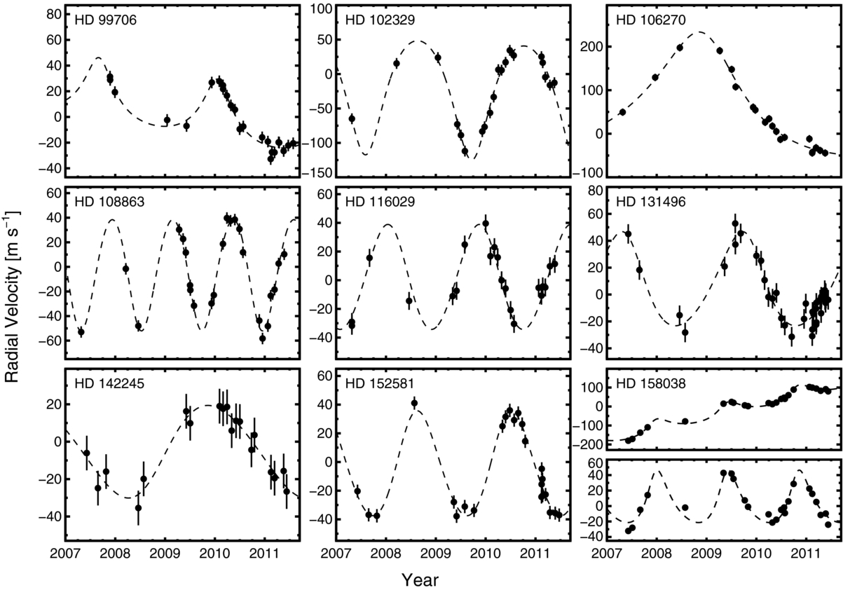
We also use the MCMC-derived pdf for the velocity trend parameter to estimate the probability that a trend is actually present in the data. We only adopt the model with the trend if the 99.7 percentile of the pdf lies above or below 0 m s−1 yr−1. The BIC and MCMC methods yield consistent results for the planet candidates presented in Section 3, and in many cases the RV trend is evident by visual inspection of Figures 2 and 3.

Figure 2. Relative RVs of nine stars measured at Keck Observatory. The error bars are the quadrature sum of the internal measurement uncertainties and jitter estimates. The dashed line shows the best-fitting orbit solution of a single Keplerian orbit, with a linear trend where appropriate.
Download figure:
Standard image High-resolution image
Figure 3. Relative RVs of nine stars measured at Keck Observatory. The error bars are the quadrature sum of the internal measurement uncertainties and jitter estimates. The dashed line shows the best-fitting orbit solution of a single Keplerian orbit. The split, lower-right panel shows the orbit of HD 158038 with a linear trend (top) and with the trend removed (bottom).
Download figure:
Standard image High-resolution image3. RESULTS
We have detected eighteen new Jovian planets orbiting evolved, subgiant stars. The RV time series of each host star is plotted in Figures 2 and 3, where the error bars show the quadrature sum of the internal errors and the jitter estimate as described in Section 2.5. The RV measurements for each star are listed in Tables 1–18, together with the Julian Date of observation and the internal measurement uncertainties (without jitter). The best-fitting orbital parameters and physical characteristics of the planets are summarized in Table 21, along with their uncertainties. When appropriate we list notes for some of the individual planetary systems.
Table 21. Orbital Parameters
| Planet | Period | Tpa | Eccentricityb | K | ω | MPsin i | a | Linear Trend | rms | Jitter | Nobs |
|---|---|---|---|---|---|---|---|---|---|---|---|
| (d) | (HJD−2,440,000) | (m s−1) | (deg) | (MJup) | (AU) | (m s−1 yr−1) | (m s−1) | (m s−1) | |||
| (1) | (2) | (3) | (4) | (5) | (6) | (7) | (8) | (9) | (10) | (11) | (12) |
| HD 1502 b | 431.8(3.5) | 15227(20) | 0.101(0.037) | 60.7(2.0) | 219(20) | 3.1(0.2) | 1.31(0.03) | 0 (fixed) | 10.9 | 9.4(0.7) | 51 |
| HD 5891 b | 177.11(0.32) | 15432(10) | 0.066(0.022) | 178.5(4.1) | 354(20) | 7.6(0.4) | 0.76(0.02) | −8.9(3.4) | 28.4 | 17.4(0.8) | 54 |
| HD 18742 b | 772(11) | 15200(110) | 0.120(<0.23) | 44.3(3.8) | 107(50) | 2.7(0.3) | 1.92(0.05) | 4.1(1.6) | 7.9 | 7.6(0.9) | 26 |
| HD 28678 b | 387.1(3.4) | 15517(30) | 0.168(0.070) | 33.5(2.2) | 126(30) | 1.7(0.1) | 1.25(0.03) | 0 (fixed) | 6.1 | 6.2(0.8) | 30 |
| HD 30856 b | 912(41) | 15260(150) | 0.117(<0.24) | 31.9(2.7) | 192(60) | 1.8(0.2) | 2.00(0.08) | 0 (fixed) | 5.2 | 6(1) | 16 |
| HD 33142 b | 326.6(3.9) | 15324(60) | 0.120(<0.22) | 30.4(2.5) | 143(60) | 1.3(0.1) | 1.06(0.03) | 0 (fixed) | 8.3 | 7.6(0.8) | 33 |
| HD 82886 b | 705(34) | 15200(160) | 0.066(<0.27) | 28.7(2.1) | 352(80) | 1.3(0.1) | 1.65(0.06) | 7.5(2.3) | 7.7 | 7.3(0.9) | 28 |
| HD 96063 b | 361.1(9.9) | 15260(120) | 0.03(<0.28) | 25.9(3.5) | 30(100) | 0.9(0.1) | 0.99(0.03) | 0 (fixed) | 5.4 | 6(1) | 15 |
| HD 98219 b | 436.9(4.5) | 15140(40) | 0.112(<0.21) | 41.2(1.9) | 57(30) | 1.8(0.1) | 1.23(0.03) | 0 (fixed) | 3.6 | 4(1) | 17 |
| HD 99706 b | 868(31) | 15219(30) | 0.365(0.10) | 22.4(2.2) | 4(20) | 1.4(0.1) | 2.14(0.08) | −7.4(2.0) | 3.7 | 4.6(0.9) | 24 |
| HD 102329 b | 778.1(7.5) | 15096(30) | 0.211(0.042) | 84.8(3.2) | 182(10) | 5.9(0.3) | 2.03(0.05) | 0 (fixed) | 7.2 | 6.4(1) | 20 |
| HD 106270 b | 2890(390) | 14830(390) | 0.402(0.054) | 142.1(6.9) | 15.2(4) | 11.0(0.8) | 4.3(0.4) | 0 (fixed) | 8.4 | 7.5(0.9) | 20 |
| HD 108863 b | 443.4(4.2) | 15516(70) | 0.060(<0.10) | 45.2(1.7) | 153(60) | 2.6(0.2) | 1.40(0.03) | 0 (fixed) | 5.1 | 4.9(0.9) | 24 |
| HD 116029 b | 670(11) | 15220(160) | 0.054(<0.21) | 36.6(3.1) | 40(80) | 2.1(0.2) | 1.78(0.05) | 5.3(1.6) | 6.9 | 5.8(0.9) | 21 |
| HD 131496 b | 883(29) | 16040(100) | 0.163(0.073) | 35.0(2.1) | 34(40) | 2.2(0.2) | 2.09(0.07) | 0 (fixed) | 6.3 | 6.8(0.8) | 43 |
| HD 142245 b | 1299(48) | 14760(240) | 0.09(<0.32) | 24.8(2.6) | 242(60) | 1.9(0.2) | 2.77(0.09) | 0 (fixed) | 4.8 | 5.5(0.9) | 19 |
| HD 152581 b | 689(13) | 15320(190) | 0.074(<0.22) | 36.6(1.8) | 321(90) | 1.5(0.1) | 1.48(0.04) | 0 (fixed) | 4.7 | 5.5(0.9) | 24 |
| HD 158038 b | 521.0(6.9) | 15491(20) | 0.291(0.093) | 33.9(3.3) | 335(10) | 1.8(0.2) | 1.52(0.04) | 63.5(1.5) | 4.7 | 6.1(0.9) | 24 |
Notes. Parameter values are based on a single-Keplerian fit to the RV time series. The parameter uncertainties are shown in parentheses and represent average 1σ confidence levels about the median from our MCMC analysis. When the measured eccentricity is consistent with e = 0 within 2σ, we quote the 2σ upper limit from the MCMC analysis in parentheses, preceded by a "<." aTime of periastron passage. bOne possible orbit solution is reported here. However, we do not have data covering a full orbit, and as a result there is a large family of possible solutions. See Section 3 for a note on this special case.
Download table as: ASCIITypeset image
HD 5891, HD 18742, HD 82886, HD 116029, HD 99706, and HD 158038. The orbit models for these stars include linear trends, which we interpret as additional orbital companions with periods longer than the time baseline of the observations.
HD 96063. The period of this system is very close to 1 yr, raising the spectra such that it may be an annual systematic error rather than an actual planet. However, any such annual signal would most likely be related to an error in the BC and, if present, would cause the RVs to correlate with the BC. We checked and found no such correlation between RV and BC. Further, we have never seen an annual signal with an amplitude of this magnitude in any of the several thousand targets monitored at Keck Observatory.
HD 106270. The reported orbit for this companion is long period and we only have limited phase coverage in measurements. In addition to the best-fitting, shorter-period orbit, in Figure 4 we provide a χ2 contour plot showing the correlation between P and MPsin i, similar to Figure 3 of Wright et al. (2009). The gray scale shows the minimum value of χ2 for single-planet Keplerian fits at fixed values of period and minimum planet mass. The solid contours denote locations at which χ2 increases by factors of {1, 4, 9} from inside out. The dashed contours show constant eccentricities e = {0.2, 0.6, 0.9} from left to right. For periods P < 100 yr the ≈99% upper limit on MPsin i is 20 MJup, with an extremely high eccentricity near e = 0.9. For eccentricities e < 0.6, MPsin i <13 MJup at ≈68% confidence and MPsin i <15 MJup at ≈99% confidence. Given the rarity of known planets with MPsin i >10 MJup around stars with masses M⋆ < 2 M☉, it is likely that the true mass of HD 106270 b is near or below the deuterium-burning limit (Spiegel et al. 2011).

Figure 4. Illustration of possible periods and minimum masses (MPsin i) for the companion orbiting HD 106270. At each value of MPsin i and P on the grid, the minimum χ2 is shown in gray scale. The solid contours denote the levels at which χ2 increases by 1, 4, and 9 with respect to the minimum, from inside out. The dashed contours denote constant eccentricity values of e = {0.2, 0.6, 0.9} from left to right.
Download figure:
Standard image High-resolution image
HD 1502, HD 5891, HD 33142. These stars exhibit RV scatter well in excess of the mean jitter value of 5 m s−1 reported by Johnson et al. (2010d). In all cases the excess scatter may be due to additional orbital companions. However, periodograms of the residuals about the best-fitting Keplerian models reveal no convincing additional periodicities. Examination of the residuals of HD 5891 shows that the tallest periodogram peaks are near 30 days and 50 days, with both periodicities below the 1% false-alarm probability (FAP) level. For the residuals of HD 33142 there is a strong peak near P = 900 days with FAP =0.8%. HD 1502 similarly shows a strong peak near 800 days with FAP ∼1%. Additional monitoring is warranted for these systems, as well as those with linear RV trends.
4. SUMMARY AND DISCUSSION
We have reported precise Doppler-shift measurements of eighteen subgiant stars, revealing evidence of Jovian-mass planetary companions. The host stars of these planets span a wide range of masses and chemical composition and thereby provide additional leverage for studying the relationships between the physical characteristics of stars and their planets. Evolved intermediate-mass stars (M⋆ > 1.5 M☉) have proven to be particularly valuable in this regard, providing a much-needed extension of exoplanet discovery space to higher stellar masses than can be studied on the main sequence, while simultaneously providing a remarkably large windfall of giant planets.
The 18 new planets announced herein further highlight the differences between the known population of planets around evolved, intermediate-mass stars and those found orbiting Sun-like stars. The initial discoveries of planets around retired A-type stars revealed a marked decreased occurrence of planets inward of 1 AU. Indeed, there are no planets known to orbit between 0.1 AU and 0.6 AU around stars with M⋆ > 1.5 M☉.
The large number of detections from our sample is a testament to the planet-enriched environs around stars more massive than the Sun. Johnson et al. (2010a) used the preliminary detections of the planets announced in this contribution, along with the detections from the CPS Doppler surveys of less massive dwarf stars, to measure the rate of planet occurrence versus stellar mass and metallicity. They found that at fixed metallicity, the number of stars harboring a gas giant planet (MPsin i ≳ 0.5 MJup) with a < 3 AU rises approximately linearly with stellar mass. And just as had been measured previously for Sun-like stars (Gonzalez 1997b; Santos et al. 2004; Fischer & Valenti 2005), Johnson et al. found evidence of a planet–metallicity correlation among their more diverse sample of stars.
These observed correlations between stellar properties and giant planet occurrence provide strong constraints for theories of planet formation. Any successful formation mechanism must not only describe the formation of the planets in our solar system but also account for the ways in which planet occurrence varies with stellar mass and chemical composition. The link between planet occurrence and stellar properties may be related to the relationship between stars and their natal circumstellar disks. More massive, metal-rich stars likely had more massive, dust-enriched protoplanetary disks that more efficiently form embryonic solid cores that in turn sweep up gas, resulting in the gas giants detected today.
The correlation between stellar mass and exoplanets also points the way toward future discoveries using techniques that are complementary to Doppler detection. To identify the best targets for high-contrast imaging surveys, Crepp & Johnson (2011) extrapolated to larger semimajor axes the occurrence rates and other correlations between stellar and planetary properties from Doppler surveys. Based on their Monte Carlo simulations of nearby stars, Crepp & Johnson found that A-type stars are likely to be promising targets for next-generation imaging surveys such as the Gemini Planet Imager, SPHERE, and Project 1640 (Macintosh et al. 2006; Claudi et al. 2006; Hinkley et al. 2011). According to their simulations, the relative discovery rate of planets around A stars versus M stars will, in relatively short order, help discern the mode of formation for planets in wide (a ≳ 10 AU) orbits. For example, an overabundance of massive planets in wide orbits around A stars as compared with discoveries around M dwarfs will indicate that the same formation mechanism responsible for the Doppler-detected sample of gas giants operates at much wider separations. Thus, just as the first handful of planets discovered by Doppler surveys revealed the planet–metallicity relationship familiar today, the first handful of directly imaged planets will provide valuable insight into the stellar mass dependence of the formation of widely orbiting planets.
Additional planets from all types of planet-search programs will enlarge sample sizes and reveal additional, telling correlations and peculiarities. As the time baselines of Doppler surveys increase, planets at ever-wider semimajor axes will be discovered, revealing the populations of planets that have not moved far from their birthplaces. As Doppler surveys move outward, they will be complemented by increases in the sensitivities of direct imaging surveys searching for planets closer to their host stars and at lower and lower masses. This overlap will most likely happen the quickest around A stars, both main-sequence and retired, providing valuable information about planet formation over four orders of magnitude in semimajor axis.
We thank the many observers who contributed to the observations reported here. We gratefully acknowledge the efforts and dedication of the Keck Observatory staff, especially Grant Hill, Scott Dahm, and Hien Tran for their support of HIRES and Greg Wirth for support of remote observing. We are also grateful to the time assignment committees of NASA, NOAO, Caltech, and the University of California for their generous allocations of observing time. J.A.J. thanks the NSF Astronomy and Astrophysics Postdoctoral Fellowship program for support in the years leading to the completion of this work and acknowledges support from NSF grant AST-0702821 and the NASA Exoplanets Science Institute (NExScI). G.W.M. acknowledges NASA grant NNX06AH52G. J.T.W. was partially supported by funding from the Center for Exoplanets and Habitable Worlds. The Center for Exoplanets and Habitable Worlds is supported by the Pennsylvania State University, the Eberly College of Science, and the Pennsylvania Space Grant Consortium. G.W.H acknowledges support from NASA, NSF, Tennessee State University, and the State of Tennessee through its Centers of Excellence program. Finally, the authors wish to extend special thanks to those of Hawaiian ancestry on whose sacred mountain of Mauna Kea we are privileged to be guests. Without their generous hospitality, the Keck observations presented herein would not have been possible.
Footnotes
- *
Based on observations obtained at the W. M. Keck Observatory and with the Hobby-Ebberly Telescope at the McDonald Observatory. Keck is operated jointly by the University of California and the California Institute of Technology. Keck time has been granted by Caltech, the University of Hawaii, NASA, and the University of California.
- 9
Some studies indicate a lack of a planet–metallicity relationship among planet-hosting K giants (Pasquini et al. 2007; Sato et al. 2008b). However, a planet–metallicity correlation is evident among subgiants, which probe an overlapping range of stellar masses and convective envelope depths (Fischer & Valenti 2005; Johnson et al. 2010a; Ghezzi et al. 2010).
- 10
- 11