


ABSTRACT
We present an overview of the GHOSTS survey, the largest study to date of the resolved stellar populations in the outskirts of disk galaxies. The sample consists of 14 disk galaxies within 17 Mpc, whose outer disks and halos are imaged with the Hubble Space Telescope Advanced Camera for Surveys (ACS). In the first paper of this series, we describe the sample, explore the benefits of using resolved stellar populations, and discuss our ACS F606W and F814W photometry. We use artificial star tests to assess completeness and use overlapping regions to estimate photometric uncertainties. The median depth of the survey at 50% completeness is 2.7 mag below the tip of the red giant branch (TRGB). We comprehensively explore and parameterize contamination from unresolved background galaxies and foreground stars using archival fields of high-redshift ACS observations. Left uncorrected, these would account for 100.65 × F814W − 19.0 detections per mag per arcsec2. We therefore identify several selection criteria that typically remove 95% of the contaminants. Even with these culls, background galaxies are a significant limitation to the surface brightness detection limit which, for this survey, is typically V ∼ 30 mag arcsec−2. The resulting photometric catalogs are publicly available and contain some 3.1 million stars across 76 ACS fields, predominantly of low extinction. The uniform magnitudes of TRGB stars in these fields enable galaxy distance estimates with 2%–7% accuracy.
Export citation and abstract BibTeX RIS
1. INTRODUCTION
The favored Λ-Cold Dark Matter (ΛCDM) cosmology has met with much success in reproducing the large-scale structure of the universe (see, e.g., Springel et al. 2005; Percival et al. 2007; Komatsu et al. 2010; Reid et al. 2010). However, the paradigm has yet to be conclusively tested on small scales. Indeed, cosmological studies on the scope of individual galaxies may provide the most stringent tests of the theory.
For example, the Sloan Digital Sky Survey (SDSS; York et al. 2000; Adelman-McCarthy et al. 2008) has now more than doubled the number of known dwarf satellite galaxies around our Galaxy (Willman et al. 2005; Zucker et al. 2006; Belokurov et al. 2007a; Koposov et al. 2008; Tollerud et al. 2008). However, the dwarf-galaxy number counts still strongly disagree with the dark matter sub-halo populations predicted by ΛCDM (Klypin et al. 1999; Moore et al. 1999; Diemand et al. 2008; Springel et al. 2008). This "missing satellite" problem has sparked much debate as it places strong constraints on the nature of dark matter (e.g., Zentner & Bullock 2003; Strigari et al. 2007; Polisensky & Ricotti 2011) as well as the behavior of baryons in dark-matter potentials (e.g., Bullock et al. 2000; Ricotti & Gnedin 2005; Okamoto et al. 2010).
ΛCDM models of hierarchical formation also predict that the ongoing accretion and disruption of many of these satellite galaxies should be observable today in our own stellar halo (e.g., Bullock et al. 2001; Bullock & Johnston 2005; Font et al. 2006). Following the initial discovery of the tidally disrupted Sagittarius Dwarf galaxy (Ibata et al. 1994), increasing evidence for these remnants has indeed been found. In particular, the SDSS has now detected significant substructure in our stellar halo both spatially (Belokurov et al. 2006; Bell et al. 2008) and in metallicity space (Belokurov et al. 2007b; Carollo et al. 2007; Ivezić et al. 2008). However, these observations still leave much room for interpretation due to both limited sky coverage and a vantage point internal to the Galaxy. For instance, whether the halo is built entirely from disrupted satellites with no smooth underlying component is still unclear (Bell et al. 2008). The problem is further complicated by recent theoretical work, which has suggested that a non-trivial amount of the stellar mass in the halo could have been contributed throughout cosmic history by the ejection of stars originally formed in the host galaxy disk (Zolotov et al. 2009; Purcell et al. 2010).
In M31, these issues are being addressed through a comprehensive effort to map the entire visible stellar halo. The inner 55 kpc was first explored in the Isaac Newton Telescope Wide-Field Camera Panoramic Survey of M31, which revealed the massive infalling giant southern stream (Ibata et al. 2001; Ferguson et al. 2002). Subsequent surveys with Megacam on the Canada–France–Hawaii Telescope covered a quadrant of the halo out to ∼150 kpc with an extension to M33 at ∼200 kpc (Martin et al. 2006; Ibata et al. 2007). The remaining quadrants are currently being mapped by the Pan-Andromeda Archaeological Survey (PAndAS; McConnachie et al. 2009). These deep surveys find a rich network of filaments out to some 120 kpc. Some of this substructure has been targeted with deep Hubble Space Telescope Advanced Camera for Surveys (HST/ACS) pointings, revealing a complex composition of stellar populations, which, in contrast to our Galaxy, is indicative of substantial mixing in the M31 system (Brown et al. 2006; Richardson et al. 2008).
In the hierarchical formation paradigm of ΛCDM, stellar halos are predominantly built up from the early accretion and disruption of low-metallicity dwarf galaxies. Once they have entered the host system, these dwarfs undergo little or no active star formation. Galaxy halos therefore provide an unfettered view of early star formation in the universe as well as the merger history of the host system (e.g., Searle & Zinn 1978; Johnston et al. 1996; Helmi & White 1999; Bullock et al. 2001; Helmi 2008). Ongoing studies of the Milky Way and M31 stellar halos will thus provide some insight on new high-resolution simulations that explore the assembly of ∼L* galaxies (e.g., Cooper et al. 2010). However, with a stochastic process like hierarchical formation, our Galaxy and M31 may be atypical of the larger population. For instance, Hammer et al. (2007) have empirically argued that the accretion history of the Milky Way has been unusually quiescent in comparison to similar systems in the local universe. Thus, to further assess our understanding of galaxy formation we have undertaken the GHOSTS (Galaxy Halos, Outer disks, Substructure, Thick disks, and Star clusters) survey of 14 nearby disk galaxies.
This survey represents the largest study of resolved stellar populations in the outer envelopes of nearby disk galaxies to date. By resolving individual stars with space-borne observatories, we are able to address a number of issues that cannot be otherwise studied. Notably, integrated light observations are limited in sensitivity principally due to the sky brightness, but also flat-field non-uniformities, Milky Way cirrus emission, bright star masking, and scattered light corrections (de Jong 2008). More generally, the integrated colors are subject to degeneracies between age, metallicity, and extinction, thus preventing discrimination of the various mechanisms believed to be responsible for the formation and evolution of these systems (de Jong et al. 2007). Alternately, for galaxies beyond the Local Group, current ground-based observations of resolved stellar populations lack the required resolution to disentangle stars in regions of high density and to reject contamination from unresolved background galaxies. Although these contaminants do not prevent the detection of substantial substructure, e.g., tidal streams (Martínez-Delgado et al. 2008, 2009), they do severely compromise the measurement of faint features like the extended stellar halo.
By resolving individual stars with the HST, we can reliably distinguish very low surface brightness structures while constraining their ages and metallicities. Such data allow us to address a number of issues. For example, using the abundant red giant branch (RGB) stars as tracers of the faint underlying population, we are able to study the size and shape of the stellar halo. These structural parameters are intrinsically connected to a number of critical phases of galaxy formation, including the small-scale behavior of the primordial power spectrum of density fluctuations; the suppression of star formation in small dark-matter potentials due to reionization, where an earlier reionization epoch leads to a fainter and more concentrated halo; and how deep the baryons of accreted satellites sit in their host dark-matter potentials (Bullock & Johnston 2005; Bekki & Chiba 2005; Abadi et al. 2006). Additionally, the triaxiality of the stellar halo depends on the shape of the dark-matter halo, which is still debated. Dissipationless (dark-matter-only) simulations, and simulations that model the formation of low-mass galaxies, typically predict strongly flattened halos (Jing & Suto 2002; Bailin & Steinmetz 2005; Allgood et al. 2006; Kazantzidis et al. 2010). Conversely, simulations that model the formation of more massive galaxies find that the processes of galaxy formation back-react on the dark matter to produce more spherical halo shapes (Abadi et al. 2006; Kazantzidis et al. 2010).
The stellar halos of galaxies also constrain models accounting for the dearth of low-mass satellites. Scenarios where star formation in smaller halos may be suppressed by reionization or baryon blowout (e.g., Bullock et al. 2000) predict that the ratio of the stellar-halo luminosity to the total luminosity of the system varies strongly with the dark-matter halo mass: from large intra-cluster light fractions for galaxy clusters, to smaller halo light fractions around our L* targets, to perhaps nearly non-existent stellar halos for our low-mass targets (Purcell et al. 2007). By covering a range of galaxy masses and morphological types, we will fully assess these predictions.
Studying resolved stellar populations also allows us to compare and contrast the metallicity of any companion dwarf galaxies and globular clusters with that of the host galaxy. Furthermore, the metallicity distribution of the host system can be studied both as a function of galaxy type and as a function of position within the galaxy. As substructure is more readily identified in the outer regions (Johnston et al. 2008), we can thus place limits on the presence of a uniform low-metallicity halo beneath the remnants of recent accretion events.
Ongoing accretion is often manifest as distinct spatial structure such as tidal streams. Studying resolved stellar populations allows us to detect these features at very faint limits. Additionally, by resolving ages and metallicities in the thin and thick disks we can study the impact of such accretion events on the host galaxy disk. This includes phenomena such as disk heating, disk truncations, and disk flaring (e.g., van der Kruit & Searle 1981; Kazantzidis et al. 2008; Purcell et al. 2010).
Future GHOSTS papers will explore all these features in depth. In particular, forthcoming papers will discuss the luminosity and density distributions of the stellar halo, bulge, and thick disk; stellar-halo substructure; stellar-halo color distributions; disk truncations; star clusters; and substructure in the M83 outer disk. This paper however focuses on a detailed description of the survey and data reduction procedures. Accordingly, we present in Section 2 the sample and our observations. Section 3 provides a discussion of the data reduction and our assessment of photometric errors. The survey completeness, the effects of contaminants, and the results of artificial star tests are presented in Section 4. Our artificial star tests are also used to define the selection criteria for the stars in the survey. The color–magnitude diagrams (CMDs) presented in Section 5 are then used to measure the tip of the red giant branch (TRGB) distances listed in Section 6. The final data products are collected in Section 7 and we summarize the survey in Section 8.
2. SAMPLE SELECTION
The GHOSTS survey began with our HST Cycle 12 SNAPshot program 9765 to study the dust structure of nearby edge-on galaxies (Seth et al. 2005a, 2005b). The quality of the observations allowed us to investigate the properties of both the thin and thick disks of the galaxies as well as the innermost volume of their stellar halos (Seth et al. 2005b). In HST Cycles 14 (SNAP program 10523) and 15 (General Observer program 10889), we extended these observations farther out into the stellar halos and expanded the sample to cover a range of galaxy masses, luminosities, inclinations, and morphological types.
Our Cycle 14 sample consists of all undisturbed disk galaxies in the list of Karachentsev et al. (2003c) with distances between 1 and 5 Mpc with low galactic foreground extinction (AV < 0.3 mag) and rotation velocities in the HyperLeda database (Paturel et al. 2003) greater than 90 km s−1. Given the short exposure times of HST SNAPshot observations, this distance limit allows us to reach a signal-to-noise ratio (S/N) >10 at one magnitude below the TRGB.
For Cycle 15 we targeted edge-on galaxies (i > 87°) in order to study halos uncontaminated by disk stars and to avoid uncertainties due to projection effects when investigating halo structure. This edge-on configuration also allows us to study thick disks and associated globular clusters. As the likelihood of observing disk galaxies at such high inclinations is low, they are typically observed at distances greater than the limits of the Karachentsev et al. (2003c) catalog and so require longer exposures. We therefore selected all undisturbed edge-on disk galaxies with rotation velocities larger than 80 km s−1, AV < 0.5 mag, and distance moduli less than 30.75 (∼14.1 Mpc). We also required at least one reliable distance estimate for each target galaxy, besides a Hubble flow distance (e.g., based on Cepheids, surface brightness fluctuations (SBFs), or accurate Tully–Fisher calibrations). In spite of these requirements, our subsequent observations showed that two of our target systems resided beyond our distance limit. Specifically, the Tully et al. (2009) Extragalactic Distance Database recorded a distance modulus (μ) of 30.64 ± 0.35 for NGC 5907, while SBF measurements of NGC 7814 have consistently measured μ < 30.75 (Tonry et al. 2001; Jensen et al. 2003). The measurements presented in Section 6 place these systems at μ = 31.13 ± 0.10 and 30.80 ± 0.10, respectively.
Data from our Cycle 12 survey of dust lanes in edge-on galaxies were added to the GHOSTS survey for those galaxies with Vrot > 80 km s−1 that were close enough to resolve stars one magnitude below the TRGB. For each of these galaxies observed during Cycles 12, 14, and 15, we also searched the Multimission Archive at STScI12 (MAST) for additional archived fields with similar exposures in both the F606W and F814W filters. Note that due to a guide-star acquisition failure, the World Coordinate System (WCS) for the archive field NGC 5236-Field 11 is incorrect in the original MAST repository. We have thus updated the WCS using the IRAF commands ccmap and ccsetwcs to fix the drizzled image to stars listed in the USNO-A2.0 Catalog (Monet 1998). The resulting astrometry is good to ∼0 4. Table 1 lists the key properties of the 14 galaxies in the GHOSTS survey and the number of suitable ACS/WFC fields available for each.
Table 1. Details of the 14 Disk Galaxies Selected for the GHOSTS Survey
| Name | α (J2000) | δ (J2000) | b | μ | D | AV | Incl. | Vrot | Morphological | Number of ACS Fields | |
|---|---|---|---|---|---|---|---|---|---|---|---|
| Angle | Type | GHOSTS | Archival | ||||||||
| (h m s) | (d m s) | (°) | (mag) | (Mpc) | (km s−1) | ||||||
| (1) | (2) | (3) | (4) | (5) | (6) | (7) | (8) | (9) | (10) | (11) | (12) |
| NGC 7814d | 00 03 14.89 | +16 08 43.5 | −45.17 | 31.1 | 17.2 | 0.15 | 70 6 6 |
231 | SA(s)ab | 5 | 0 |
| NGC 0253e | 00 47 33.12 | −25 17 17.6 | −87.96 | 27.5 | 3.2 | 0.06 | 780 |
194 | SAB(s)c | 5 | 5 |
| NGC 0891ab | 02 22 33.41 | +42 20 56.9 | −17.41 | 30.0 | 10.2 | 0.28 | 880 |
212 | SA(s)b | 2 | 3 |
| NGC 2403de | 07 36 51.40 | +65 36 09.2 | 29.19 | 27.7 | 3.6 | 0.13 | 600 |
122 | SAB(s)cd | 7 | 0 |
| NGC 3031 (M 81)bcde | 09 55 33.17 | +69 03 55.1 | 40.90 | 27.8 | 3.7 | 0.27 | 590 |
225 | SA(s)ab | 6 | 6 |
| NGC 4244ade | 12 17 29.66 | +37 48 25.6 | 77.16 | 28.3 | 4.7 | 0.07 | 880 |
89 | SA(s)cd | 8 | 0 |
| NGC 4565ad | 12 36 20.78 | +25 59 15.6 | 86.44 | 30.6 | 13.3 | 0.05 | 900 |
245 | SA(s)b | 4 | 0 |
| NGC 4631cde | 12 42 08.01 | +32 32 29.4 | 84.22 | 29.1 | 6.7 | 0.06 | 850 |
139 | SB(s)d | 2 | 0 |
| NGC 4736 (M 94)de | 12 50 53.06 | +41 07 13.7 | 76.01 | 28.5 | 5.0 | 0.06 | 350 |
167 | (R)SA(r)ab | 3 | 0 |
| NGC 5023de | 13 12 12.60 | +44 02 28.4 | 72.58 | 29.8 | 9.5 | 0.06 | 900 |
80 | Scd | 1 | 0 |
| NGC 5236 (M 83)be | 13 37 00.95 | −29 51 55.5 | 31.97 | 28.3 | 4.7 | 0.22 | 463 |
164 | SAB(s)c | 4 | 8 |
| NGC 5907bd | 15 15 53.77 | +56 19 43.6 | 51.09 | 31.1 | 16.5 | 0.04 | 870 |
227 | SA(s)c | 1 | 0 |
| IC 5052ae | 20 52 01.63 | −69 11 35.9 | −35.80 | 29.5 | 8.1 | 0.17 | 900 |
80 | SBd | 2 | 0 |
| NGC 7793ae | 23 57 49.83 | −32 35 27.7 | −77.17 | 28.2 | 4.4 | 0.07 | 530 |
96 | SA(s)d | 4 | 0 |
Notes. Key to columns: (1) NGC/IC and Messier identifier; (2) and (3) right ascension and declination; (4) Galactic latitude in degrees; (5) and (6) approximate distance modulus, and distance to the galaxy in Mpc, as listed in the NASA/IPAC Extragalactic Database (NED; http://nedwww.ipac.caltech.edu) as of 2011 February 1; (7) V-band Galactic extinction from Schlegel et al. (1998); (8) inclination angle of the galaxy, as listed in HyperLeda (Paturel et al. 2003, http://leda.univ-lyon1.fr); (9) rotational velocity in km s−1 (HyperLeda); (10) morphological type (NED); (11) number of HST (ACS WFC) fields taken for each galaxy as part of the GHOSTS survey; (12) number of HST (ACS WFC) fields of sufficient depth and with F606W and F814W observations available in the HST archive (MAST). aThis system has a known disk truncation. bThis system is known to have significant stellar tidal features. cH i studies have revealed this galaxy to be part of an interacting system. dThis system was imaged by SDSS. eThis system was imaged with Spitzer/IRAC by the Spitzer Infrared Nearby Galaxies (SINGS; Kennicutt et al. 2003) or Local Volume Legacy (LVL; Dale et al. 2009) surveys.
Download table as: ASCIITypeset image
2.1. HST/ACS Observations
Tiling the entire contiguous stellar halo of each galaxy with ACS Wide Field Channel (WFC) imaging is not feasible. Instead, we spaced several fields along the major and minor axes of each galaxy, principally to measure the halo structure. For highly inclined systems, a few additional fields were placed on an intermediate axis for sensitivity to deviations from elliptical isophotes and to track the metallicity as a function of disk scale height. This strategy allowed us both to cover a broad variety of galaxies and to probe the stellar halos out to large radii. The precise field locations are chosen to avoid bright foreground stars, to allow HST to use all available roll angles, and to sample known features, such as disk truncations and previously identified stellar streams. Consequently, as the target fields are not placed randomly, caution should be used when assessing the statistical significance and frequency of features such as tidal streams.
RGB stars are the most luminous and numerous stars among the old stellar populations that are expected to dominate the GHOSTS halo fields. Imaging was thus obtained in the F814W filter, where the flux of these stars peaks, together with the F606W filter for color discrimination. Compared to the longer wavelength baselines available with other ACS filter choices, F606W and F814W imaging maximizes throughput in a single orbit at the expense of some loss in color sensitivity. This greater depth vastly improves our statistics in the sparsely populated stellar halos, which, when studying cumulative populations, more than compensates for the increased error in individual stellar-color estimates.
For the SNAPshots in Cycles 12 and 14, we targeted each field with a single orbit of approximately 45 minutes. Two exposures for each filter were taken to remove the effects of cosmic rays. Total exposure times were typically 700 s in each filter, to reach the required S/N =10 at 1 mag below the TRGB. The GO program in Cycle 15 allowed us to go deeper and so extend our sample to more distant edge-on galaxies. Exposure times for these systems were chosen to achieve the same S/N in all sources, giving total exposure times of 7350 and 7192 s in the F606W and F814W filters for what we believed to be our most distant galaxy, NGC 4565. These observations were dithered to remove the chip gap and to increase the sampling of the detector. Observations with the Wide Field Planetary Camera 2 (WFPC2) and the Near-Infrared Camera and Multi-Object Spectrometer (NICMOS) were taken in parallel where available for tertiary science goals. Data from these instruments will be presented separately.
Unfortunately, the ACS failure in 2007 January meant that our Cycle 15 observing program could not be completed as planned. However, the program was extended with WFPC2, the results of which will also be presented in a later paper. The new and archival ACS observations for this survey are summarized in Table 2.
Table 2. HST/ACS Observations
| Galaxy | Field | Proposal | R.A. | Decl. | Position | Observation | Coverage | Total Exposure Times (s) | |
|---|---|---|---|---|---|---|---|---|---|
| ID | Angle | Date | F606W | F814W | |||||
| (h m s) | (° m s) | (°) | (arcsec2) | ||||||
| (1) | (2) | (3) | (4) | (5) | (6) | (7) | (8) | (9) | (10) |
| NGC 7814 | Field-01a | 10889 | 00 03 12.41 | 16 07 34.99 | 30.16 | 2006 Aug 26 | 39357 | 5211(5) | 5215(5) |
| Field-02a | 10889 | 00 03 24.31 | 16 05 58.09 | 25.98 | 2006 Sep 13 | 39803 | 5211(5) | 5215(5) | |
| Field-03 | 10889 | 00 03 11.45 | 16 08 42.57 | 46.96 | 2006 Jul 24 | 39451 | 5211(5) | 5215(5) | |
| Field-04 | 10889 | 00 02 59.24 | 16 04 11.75 | 27.99 | 2006 Sep 12 | 39488 | 5211(5) | 5215(5) | |
| Field-05 | 10889 | 00 03 15.34 | 16 04 17.55 | 22.99 | 2006 Sep 15 | 39266 | 5211(5) | 5215(5) | |
| NGC 0253 | Field-01ab | 10915 | 00 47 36.33 | −25 16 44.20 | 139.99 | 2006 Sep 13 | 41053 | 1508(2) | 1534(2) |
| Field-02ab | 10915 | 00 47 47.07 | −25 14 44.85 | 140.89 | 2006 Sep 9 | 41417 | 1508(2) | 1534(2) | |
| Field-03ab | 10915 | 00 47 57.81 | −25 12 45.49 | 159.22 | 2006 Sep 15 | 41695 | 1508(2) | 1534(2) | |
| Field-04ab | 10915 | 00 48 08.55 | −25 10 46.13 | 139.99 | 2006 Sep 8 | 41822 | 1508(2) | 1534(2) | |
| Field-05ab | 10915 | 00 48 19.29 | −25 08 46.78 | 144.99 | 2006 Sep 19 | 37890 | 2283(3) | 2253(3) | |
| Field-06c | 10523 | 00 48 35.52 | −25 05 17.17 | 51.04 | 2006 May 19 | 40055 | 680(2) | 680(2) | |
| Field-07c | 10523 | 00 48 55.48 | −25 00 37.71 | 113.61 | 2005 Sep 1 | 40060 | 680(2) | 680(2) | |
| Field-08c | 10523 | 00 47 13.93 | −25 10 10.71 | 60.16 | 2006 Jun 13 | 40149 | 680(2) | 680(2) | |
| Field-09c | 10523 | 00 47 45.03 | −25 22 11.25 | 134.80 | 2005 Sep 13 | 40164 | 680(2) | 680(2) | |
| Field-10c | 10523 | 00 47 22.95 | −25 25 42.15 | 190.72 | 2005 Oct 24 | 40002 | 680(2) | 680(2) | |
| NGC 0891 | Field-01abc | 9414 | 02 22 42.74 | 42 19 42.40 | 244.00 | 2003 Feb 18 | 39189 | 7711(9) | 7711(9) |
| Field-02abc | 9414 | 02 22 49.74 | 42 22 49.20 | 244.28 | 2004 Jan 17 | 37157 | 7711(9) | 7711(9) | |
| Field-03a | 9765 | 02 22 38.84 | 42 24 15.81 | 244.02 | 2004 Feb 18 | 41347 | 676(2) | 700(2) | |
| Field-04abc | 9414 | 02 22 56.64 | 42 25 55.10 | 244.62 | 2004 Feb 17 | 39152 | 7711(9) | 7711(9) | |
| Field-05 | 10889 | 02 22 36.56 | 42 20 50.59 | 17.23 | 2006 Oct 22 | 39284 | 3170(3) | 3080(3) | |
| NGC 2403 | Field-01ab | 10182 | 07 36 57.22 | 65 36 21.53 | 140.03 | 2004 Aug 17 | 34477 | 700(2) | 700(2) |
| Field-02ac | 10523 | 07 37 52.70 | 65 31 30.99 | 107.68 | 2005 Sep 29 | 39298 | 710(2) | 710(2) | |
| Field-03c | 10523 | 07 38 24.40 | 65 28 08.40 | 115.39 | 2005 Sep 18 | 39818 | 740(2) | 745(2) | |
| Field-04ac | 10523 | 07 39 02.01 | 65 24 43.50 | 87.06 | 2005 Oct 29 | 40021 | 735(2) | 735(2) | |
| Field-05c | 10523 | 07 37 29.37 | 65 40 29.13 | 97.84 | 2005 Oct 14 | 39908 | 720(2) | 720(2) | |
| Field-06c | 10523 | 07 37 59.69 | 65 43 43.58 | 72.88 | 2005 Nov 15 | 39979 | 745(2) | 745(2) | |
| Field-07c | 10523 | 07 39 11.22 | 65 37 32.63 | 126.54 | 2005 Sep 4 | 39932 | 730(2) | 730(2) | |
| NGC 3031 | Field-01ab | 9353 | 09 55 25.00 | 69 01 13.00 | 272.80 | 2002 May 28 | 35640 | 834(2) | 1671(3) |
| Field-02ab | 10915 | 09 54 34.71 | 69 16 49.76 | 89.81 | 2006 Nov 16 | 21988 | 24232(10) | 29953(12) | |
| Field-03c | 10523 | 09 54 23.12 | 69 19 56.41 | 84.98 | 2005 Dec 6 | 40050 | 700(2) | 700(2) | |
| Field-04c | 10523 | 09 53 59.63 | 69 24 58.57 | 120.26 | 2005 Oct 26 | 40148 | 720(2) | 720(2) | |
| Field-05c | 10523 | 09 57 17.23 | 69 06 29.27 | 117.09 | 2005 Oct 31 | 40075 | 710(2) | 710(2) | |
| Field-06c | 10523 | 09 58 04.50 | 69 08 52.15 | 117.32 | 2005 Oct 31 | 40136 | 735(2) | 735(2) | |
| Field-07c | 10523 | 09 58 52.30 | 69 10 42.12 | 162.14 | 2005 Sep 7 | 40252 | 730(2) | 730(2) | |
| Field-08c | 10523 | 09 56 39.13 | 69 22 29.58 | 70.09 | 2005 Dec 20 | 40299 | 740(2) | 740(2) | |
| Field-09abc | 10136 | 09 54 16.54 | 69 05 35.71 | 297.00 | 2005 Apr 13 | 20356 | 5354(4) | 5501(4) | |
| Field-10ab | 10584 | 09 56 28.24 | 68 54 39.74 | 69.76 | 2005 Dec 9 | 40047 | 1580(3) | 1595(3) | |
| Field-11ab | 10584 | 09 57 00.92 | 68 55 53.49 | 69.77 | 2005 Dec 6 | 40868 | 1580(3) | 1595(3) | |
| Field-12b | 10604 | 09 53 03.20 | 68 52 03.60 | 160.12 | 2005 Sep 11 | 39191 | 12470(10) | 22446(18) | |
| NGC 4244 | Field-01a | 9765 | 12 17 30.24 | 37 48 07.67 | 133.60 | 2003 Nov 12 | 41335 | 676(2) | 700(2) |
| Field-02ac | 10523 | 12 17 43.76 | 37 50 36.82 | 120.87 | 2005 Dec 24 | 40114 | 720(2) | 720(2) | |
| Field-03ac | 10523 | 12 17 56.15 | 37 53 16.13 | 136.78 | 2005 Nov 10 | 40227 | 730(2) | 730(2) | |
| Field-04c | 10523 | 12 18 13.30 | 37 56 25.72 | 133.52 | 2005 Nov 15 | 40176 | 750(2) | 750(2) | |
| Field-05c | 10523 | 12 18 34.65 | 37 59 21.30 | 137.74 | 2005 Nov 9 | 39996 | 710(2) | 710(2) | |
| Field-06c | 10523 | 12 17 40.54 | 37 46 38.93 | 131.88 | 2005 Nov 22 | 40112 | 735(2) | 735(2) | |
| Field-07c | 10523 | 12 17 53.83 | 37 44 02.01 | 133.03 | 2005 Nov 15 | 40150 | 375(1) | 375(1) | |
| Field-08ac | 10523 | 12 17 06.69 | 37 44 25.53 | 141.09 | 2005 Nov 4 | 40409 | 700(2) | 700(2) | |
| NGC 4565 | Field-01a | 10889 | 12 36 25.66 | 26 00 58.09 | 119.16 | 2006 Dec 13 | 39673 | 7350(7) | 7192(7) |
| Field-02a | 10889 | 12 36 35.99 | 25 58 14.82 | 118.01 | 2006 Dec 11 | 39803 | 7350(7) | 7192(7) | |
| Field-03 | 10889 | 12 36 40.88 | 26 04 12.35 | 118.78 | 2006 Dec 13 | 39670 | 7350(7) | 7192(7) | |
| Field-04a | 9765 | 12 36 07.36 | 26 01 56.87 | 337.78 | 2004 Apr 15 | 41612 | 676(2) | 700(2) | |
| NGC 4631 | Field-01a | 9765 | 12 42 08.20 | 32 32 56.88 | 268.28 | 2003 Aug 3 | 40711 | 676(2) | 700(2) |
| Field-02a | 9765 | 12 41 51.55 | 32 32 23.15 | 301.21 | 2004 Jun 9 | 44972 | 676(2) | 700(2) | |
| NGC 4736 | Field-01ac | 10523 | 12 51 14.24 | 41 03 59.87 | 98.53 | 2006 Jan 22 | 39918 | 730(2) | 730(2) |
| Field-02c | 10523 | 12 51 33.61 | 41 00 26.55 | 148.06 | 2005 Nov 7 | 40150 | 750(2) | 850(2) | |
| Field-03c | 10523 | 12 51 26.81 | 41 15 51.74 | 102.79 | 2006 Jan 8 | 40142 | 740(2) | 740(2) | |
| NGC 5023 | Field-01a | 9765 | 13 12 13.69 | 44 02 15.80 | 290.04 | 2004 Jul 2 | 41682 | 400(1) | 676(2) |
| NGC 5236 | Field-01abc | 9864 | 13 37 01.70 | −29 43 52.00 | 296.58 | 2004 Aug 10 | 37437 | 1900(2) | 3000(2) |
| Field-02ab | 10608 | 13 36 55.15 | −29 41 49.85 | 305.99 | 2006 Jul 23 | 40859 | 1190(2) | 890(2) | |
| Field-03cd | 10523 | 13 36 47.99 | −29 36 54.93 | 223.51 | 2006 Apr 30 | 39839 | 740(2) | 740(2) | |
| Field-04c | 10523 | 13 37 07.62 | −29 34 57.76 | 219.01 | 2006 Apr 29 | 39879 | 730(2) | 730(2) | |
| Field-05cd | 10523 | 13 36 44.01 | −29 33 11.54 | 222.14 | 2006 Apr 30 | 39838 | 750(2) | 750(2) | |
| Field-06bc | 10235 | 13 36 30.80 | −29 14 11.00 | 265.41 | 2005 May 25 | 39355 | 1200(2) | 900(2) | |
| Field-07ac | 10523 | 13 36 28.07 | −29 54 09.90 | 219.02 | 2006 Apr 29 | 39829 | 725(2) | 725(2) | |
| Field-08b | 10608 | 13 35 56.02 | −29 57 23.02 | 122.95 | 2006 Feb 22 | 41124 | 1190(2) | 890(2) | |
| Field-09bc | 10235 | 13 35 08.10 | −30 07 04.00 | 288.91 | 2005 Jul 14 | 39371 | 1200(2) | 900(2) | |
| Field-10b | 10608 | 13 35 43.01 | −29 43 48.80 | 122.78 | 2006 Feb 22 | 41279 | 1190(2) | 890(2) | |
| Field-11b | 10608 | 13 36 56.90 | −30 06 41.73 | 101.93 | 2005 Dec 25 | 40776 | 1198(2) | 898(2) | |
| Field-12b | 10608 | 13 37 00.74 | −30 07 30.39 | 306.33 | 2006 Jul 24 | 41088 | 1198(2) | 898(2) | |
| NGC 5907 | Field-01a | 10889 | 15 17 00.13 | 56 20 39.81 | 123.12 | 2007 Jan 10 | 40081 | 5661(6) | 5616(6) |
| IC 5052 | Field-01a | 9765 | 20 52 03.45 | −69 12 23.96 | 298.30 | 2003 Dec 14 | 43532 | 676(2) | 700(2) |
| Field-02 | 10889 | 20 51 33.61 | −69 14 10.75 | 173.14 | 2006 Jul 28 | 39882 | 1789(2) | 1760(2) | |
| NGC 7793 | Field-01ac | 10523 | 23 58 20.17 | −32 35 54.40 | 130.14 | 2005 Sep 5 | 40127 | 740(2) | 740(2) |
| Field-02c | 10523 | 23 58 37.09 | −32 36 36.78 | 51.91 | 2006 May 14 | 40102 | 730(2) | 730(2) | |
| Field-03c | 10523 | 23 57 53.02 | −32 29 13.90 | 86.56 | 2005 Jul 19 | 40003 | 750(2) | 750(2) | |
| Field-04c | 10523 | 23 57 57.20 | −32 25 43.65 | 49.93 | 2006 May 10 | 40153 | 720(2) | 720(2) | |
Notes. Key to columns: (1) NGC/IC and Messier identifier; (2) field identifier. Fields are numerically labeled outward, first along one side of the major axis, then along one side of the minor axis, then any intermediate axes before labeling remaining fields by distance from the galaxy center; (3) HST proposal ID of the observation; (4) and (5) right ascension and declination; (6) the HST PA_V3 angle, which records the projected angle on the sky eastward of north that the observatory was rotated; (7) observation date; (8) area covered by the field in arcsec2 after masking for bad pixels and extended objects (see Section 3.2); (9) and (10) the total time of the exposure in seconds for the F606W and F814W filters. The number of exposures in each filter is indicated in brackets. aSignificant stellar crowding in these fields results in a loss of stellar detections as individual stars may no longer be resolved. This can generally be corrected for by using the artificial star tests described in Section 4.1. bThese fields are reduced from the Multimission Archive at the Space Telescope Science Institute (MAST). cThese observations are undithered. dThese fields are placed on a known stellar stream observed in deep optical images.
3. DATA REDUCTION
The ACS/WFC data were downloaded from the Hubble Data Archive as *_flt FITS files. These observations have already been passed through the calacs package, which performs the initial data reduction as part of the opus pipe line (see the HST Data Handbook for ACS; Gonzaga et al. 2011). More specifically, the data have been bias-subtracted, passed through an initial cosmic-ray identification routine, corrected for the dark image, and finally flat-fielded. Bad pixels have also been flagged, however we used a series of IRAF routines (namely ccdmask) to pick out any additional bad columns not previously identified. We then passed the images through a further cleaning step, masked out extended sources, and finally performed the photometry.
3.1. Drizzling
To combine individual CCD frames into a distortion-corrected image, we used the MultiDrizzle package (Koekemoer et al. 2002). By combining multiple frames, this routine identified any additional cosmic rays which were blotted back to the original *_flt files and flagged as bad pixels. The photometry was carried out on these individual CCD frames, although we used the combined, resampled FITS image as a reference frame for coordinate positions.
We followed the standard MultiDrizzle steps outlined in the manual13 (Fruchter & Sosey 2009) but initially ran TweakShifts on all the CCD images for a given target. This task computed any residual shifts between the WCS of the observations and ensured that the final drizzled images for both filters used the same coordinate system. As MultiDrizzle updates the header of the *_flt files, we also turned off sky subtraction, and correspondingly set pixfrac =1.0, to ensure proper treatment of Poissonian noise by the photometry code.
3.2. Extended Source Identification
We initially constructed a mask of all extended and resolved objects using SExtractor (Bertin & Arnouts 1996). This routine was run on the drizzled F814W image with the detection and deblending parameters set to detect extended objects without grouping individual stars together. Specifically, the source image was not smoothed (filter n) before detection, the drizzle weight image was used as a weight map (type is map_rms), and the detection threshold (detect_thresh) was deliberately set low at 1.6σ above the sky level in order to encompass the whole extended object. However, we set the analysis threshold slightly higher (analysis_thresh =2.0) to accurately compute the full width at half-maximum (FWHM). Our goal with SExtractor was not to provide a comprehensive catalog of all objects in the field but only a catalog of the extended sources. Therefore, we also set the minimum number of pixels in a detected object (detect_minarea) to 70. Our deblending parameters were deblend_nthresh =32 and deblend_mincont =0.006, ensuring moderately aggressive deblending. The resulting SExtractor run produced a catalog of all the extended objects in the F814W field and a segmentation map.
The SExtractor catalog contains structural parameters that have proven useful to separate galaxies from stars in previous work (e.g., Holwerda et al. 2005). These parameters include a simple concentration index, defined as the ratio of the peak surface brightness to the total luminosity in the pixels above 1.6σ (mu_max/mag_iso), the number of pixels in the object (isoarea_image), the ellipticity (= 1 −minor/major axis ratio), and the FWHM (fwhm_image). SExtractor's own star/galaxy classification is also included even though the procedure has not been calibrated on HST images and becomes random well above the detection limit.
In order to select only extended objects, we set a minimum to the number of pixels in each detection (isoarea_image >100). Additionally, we removed spurious detections due to stellar crowding in the main disk by excluding objects in regions of sufficient surface brightness (which is included in the GHOSTS database as a galaxy mask where applicable; see Section 7). The resulting segmentation mask, which maps the extended objects, was then passed through a maximum filter (7 × 7 pixels in size) to pad the mask for each extended object. This padding ensures that detections which lie on the periphery of an extended object are removed, as typically these detections are associated with the extended object itself. These padded-masked regions are excluded from all further analysis.
During the initial photometry stages, it was observed that the photometry code was less effective at detecting sources within the halos of bright foreground stars. In fields far from the main galaxy disk, this effect can be corrected by artificial star tests (see Section 4.1). However, this is not necessarily the case in fields where bright regions are not only due to the halos of these foreground stars but also due to the galaxy disk itself. To ensure this effect did not impinge upon our results, we excluded by hand a larger region surrounding these few foreground stars. These regions are included in the segmentation map to ensure proper calculation of the survey window.
3.3. Photometry
We used the ACS module of dolphot (Dolphin 2000, a modified version of HSTphot) to identify stars and for photometric measurements. This code initially uses a library of precomputed Tiny Tim point-spread functions (PSFs) to center and measure the magnitude of each star in both filters. The code was run on the flat-fielded CCD images (*_flt), which have been masked for bad pixels (e.g., hot pixels, cosmic rays, bad columns, etc.) as described earlier. We configured dolphot with parameters similar to those used in the ACS Nearby Galaxy Survey Treasury program (Dalcanton et al. 2009, hereafter ANGST).
dolphot initially aligns the dithered exposures using bright stars in common between the frames; generally, the alignment is good to ∼001 precision. The code then scans for stars by searching for peaks in image brightness after subtracting the background sky, chosen here as the region bound between the photometry aperture and the PSF. For completeness, a second pass is made with the previous identifications subtracted from the image. dolphot then iteratively solves for the magnitude of each detected star by accounting for the photometry of neighboring stars at each step. During this process the flux is computed by simply scaling the PSF. As the photometry of faint stars is dependent on the shape of the assumed PSF, dolphot modifies the reference PSFs by minimizing the residuals of bright, isolated stars. This step is computed only after a reasonable convergence of all stellar magnitudes is achieved. Overall, ANGST found that these deviations affect the final photometry on the order of 0.01 mag.
Aperture corrections to the PSF magnitudes were calculated and applied by dolphot using isolated stars. Typically, these were found to be <0.05 mag. The code also implements the latest corrections for charge transfer efficiency (CTE) loss using the CTE analytical expressions given in the Instrument Science Report ACS-ISR 2009-01 (Chiaberge et al. 2009). For this survey, CTE corrections typically increase from zero at the chip edge to 0.08 mag at the chip center.
The final output lists the position of each star relative to the drizzled image, together with the measured magnitudes and a slew of diagnostic data for the combined image, as well as for the individual exposures. These include the χ2 for the fit to the PSF; an S/N value; sharpness, which can be used to discriminate detections that are either too sharp, such as cosmic rays and hot pixels, or too broad, i.e., background galaxies; roundness, which is used to detect extended or diffracted objects; and crowding, which indicates the change in brightness if nearby stars were not simultaneously fit. Also, the output for each detection are the more general parameters of object type and error flag. The former describes the general shape of the detection, while the latter indicates any issues with the fit, including the presence of bad or saturated pixels. Magnitudes are calculated in ST Instrumental VEGA magnitudes as well as Johnson–Cousins equivalent values using the transformations described in Sirianni et al. (2005). The code also used the latest zero points reported on the STScI Web site.14 These are separately quoted for data taken before and after the ACS anomaly in 2006 June, which led to an increase in operating temperature after the switch to side-2 electronics.
dolphot was executed with a number of user-defined parameters that primarily affect the star fitting, sky fitting, and aperture correction routines. These parameters were investigated in depth by ANGST and for crowded regions we have adopted their values. Most notably, setting Fitsky = 3 simultaneously fits the sky and the star PSF as a two-parameter fit within a reasonably large aperture of radius (rAper =) 10 pixels. However, to ensure the code runs reliably in crowded regions with these settings, the Force1 flag needs to be set, such that all detections are treated as stars, regardless of the morphology of the object. For our sparser fields, we found these settings resulted in too many contaminants relative to the true number of stars (see Section 4.2). We therefore re-ran dolphot on all fields with Force1 set to off in order to fit only the most likely candidates. Correspondingly, to ensure the most robust fitting in the sparser regions, albeit with a greater noise level in the crowded fields, we used a smaller photometry aperture (rAper = 4 pixels) and set Fitsky = 2, which fits the sky outside the photometry aperture but within the PSF. We thus produced catalogs using both prescriptions for all fields. The two methods produced similar results in regions of intermediate density that are neither sparse nor crowded.
To test the reliability of the dolphot output, we present in Figure 1 a comparison of the photometry carried out on Fields 01 and 02 of NGC 5236 using the parameters for sparse fields. These fields overlap by approximately 18%, with some 2500 RGB stars in common. For coincident detections, we plot the difference in magnitudes reported by dolphot for both filters up to the ∼50% completeness limit. Also plotted are binned means, with error bars indicating the 1σ spread in the scatter. These are to be compared with the shaded regions that denote the mean expected error, computed for each pair by combining in quadrature the dolphot error for both measurements.

Figure 1. Comparison of the dolphot photometry for overlapping stars in Fields 01 and 02 of NGC 5236. Darker symbols indicate the mean offset of the uncertainty in bins of ∼0.13 mag, with error bars indicating the 1σ spread. Shaded regions denote the expected 1σ uncertainty by combining in quadrature the dolphot reported error of each detection as a function of magnitude. Generally, the spread of the data points is comparable to the dolphot errors.
Download figure:
Standard image High-resolution imageIn each case the observed distribution is consistent with the dolphot errors, although a small offsets of −0.04 mag is found in the F814W filter. This offset is similar to the average CTE correction applied by dolphot to each star. However, when comparing corrections between chips, as we have done here, Chiaberge et al. (2009) find that CTE corrections may overcorrect, leading to an apparent offset of up to ∼0.05 mag. This is similar to the error arising from not correcting for CTE, but in the opposite sense. Hence this may be the cause of the offset noted here. Alternatively, the offset may be due to variances in the focus due to thermal heating of the observatory (known as "breathing"), although dolphot does attempt to account for this. Finally, the difference may be caused by aperture corrections, as the stars chosen to measure these residuals will be different in each field. Regardless, we note that although the offset is statistically significant, the magnitude of the difference is substantially less than the typical uncertainty reported by dolphot. We thus find the dolphot code to be photometrically reliable and accurate. Furthermore, we use the reported errors as our final total uncertainty on the measured magnitudes. This approach is shared by the ANGST survey who, through a series of photometric tests, found that any systematics in the dolphot code are dwarfed by the final errors assigned by the code. At the TRGB of our closest galaxy, NGC 2403, the average dolphot error is only 0.04 mag. This degrades to 0.22 mag at the faint limit of the survey, defined here as the 50% completeness limit, as averaged over all fields. The mean dolphot error for all stars in all fields at S/N >10 is 0.06 mag.
4. SURVEY COMPLETENESS
By equating the density of observed stars to surface brightness, we can reach extremely faint surface-brightness levels. The steps involved in this process are outlined in Figure 2. Here, a triangular region of the stellar halo of NGC 4565 denotes the area used to measure the surface brightness along the minor axis of the system. The number of stars in radial bins in this region are counted and divided by the area covered by the observation (corrected for the area lost to bright foreground stars and resolved background galaxies). In this case, RGB stars, selected by color and magnitude from the CMD, are used. These 8–12 Gyr old stars are the most readily observed and are responsible for the majority of light in these older outer regions. Then, using a least-squares algorithm, the logarithm of the stellar density is linearly offset to match a surface brightness profile extracted from an all-galaxy image of the inner region. The stellar densities for each GHOSTS field in a galaxy are offset by the same amount to ensure consistency. We find that an SDSS z-band image provides a good fit to an RGB-dominated population. However, SDSS i-band and Spitzer/IRAC 3.6μ or 4.5μ observations also provide reasonable fits with no significant differences. Galaxies in the sample that are covered by SDSS or observed with Spitzer/IRAC either through the Spitzer Infrared Nearby Galaxies (SINGS; Kennicutt et al. 2003) or Local Volume Legacy (LVL; Dale et al. 2009) surveys are identified in Table 1.
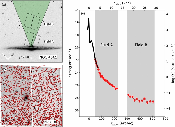
Figure 2. Minor-axis radial light profile of NGC 4565 as measured from star counts. Panel (a) plots the location of the relevant ACS WFC fields. The shaded region denotes the area used for constructing the profile. Panel (b) shows the distortion-corrected drizzled ACS/WFC observation of Field B using the F814W filter. The galaxy center is toward the bottom of the image as presented here. Detected RGB star locations are marked by dots while the lines mark the radial bins used for the profile. Panel (c) shows the radial profiles within the shaded area of panel (a), both as extrapolated from SDSS images (converted to I band; thick black line) and as measured by the stellar density in each radial bin (red points). The scale of the star counts has been linearly offset to match the SDSS profile. The dip around 1 kpc in the integrated light profile is due to the dust lane seen in panel (a). The radii covered by the two fields are marked by the shaded gray regions. Background contaminants have been subtracted and the error bars denote the combined photometric uncertainties (see Section 4.2).
Download figure:
Standard image High-resolution imageAs shown in Figure 2, there is generally good agreement between the density of RGB stars and the surface brightness as measured by SDSS. Note that the I-band magnitude plotted here is a combination of the SDSS iAB and zAB bands as described on the SDSS Web site.15 There can, however, be some disagreement in regions of high surface brightness, like the thin disk and bulge, where it can be difficult to resolve individual stars due to stellar crowding. This occurs when the PSFs of the stars overlap. We can statistically correct for this effect by populating the image with artificial stars and measuring the fraction that we successfully recover. This enables the correlation of the internal structure of the galaxy with that of the stellar halo (see Section 4.1).
Figure 2 also illustrates the great depths which resolved stellar populations enable us to reach (typically V ∼ 30 mag arcsec−2 for this survey). This limit is set by sampling statistics and the accuracy of contaminant subtraction. As we reach out into the halo, the detection rate of individual RGB stars becomes low enough that Poisson errors dwarf the signal. Ever deeper observations will reach further down the luminosity function yielding many more stars and even fainter limiting surface brightnesses. However, contamination from faint foreground stars and background unresolved galaxies often becomes the dominant source of uncertainty at such low detection limits. This is discussed further in Section 4.2.
4.1. Artificial Star Tests
Artificial star tests were carried out to assess the completeness in recovering all the stars in a given field using the dolphot package. Artificial stars were added to each field image and passed through dolphot one at a time in parallel batches. The properties of these "fake" stars, i.e., color and brightness, are chosen to mimic the observed stars, but extended to fainter magnitudes. We vary the number of artificial stars generated based on surface brightness, populating the higher surface brightness regions of an observation with more artificial stars. Typically, we computed the photometry for 500,000 to 2,000,000 artificial stars per field. The probability of recovery was then assessed as a function of the stellar magnitude in each filter as well as the local surface brightness. We can thus correct our stellar densities for the effects of crowding, where individual stars may no longer be resolved. This correction is shown in Figure 3 where the radial light profile along the major axis of NGC 4244 is plotted both before and after this correction. At the center of the galaxy, where the stars appear merged, a significant deficit in the brightness is seen. However, after correction, the surface brightness, as inferred from the stellar density, precisely matches the observed SDSS i-band photometry.

Figure 3. Major-axis radial light profiles for NGC 4244 as traced by RGB stars and detailed in de Jong et al. (2007b). The dashed line indicates the background contaminant level subtracted from the data. Panel (a) plots the measured surface brightness profile before correction with the artificial star tests. Panel (b) plots the profiles after correction. The solid black line is the surface profile of the central region as extracted from the SDSS z-band image shown in the lower panel. Panel (c) also shows the shaded GHOSTS ACS fields and the horizontal strip down the center of the galaxy, which defines the region used to construct the profiles both from the RGB counts and as measured from the SDSS image. The scale of the star counts has been linearly offset by the same amount in each panel to match the SDSS profile to the corrected star counts.
Download figure:
Standard image High-resolution imageOverall, the dolphot recovery of the input parameters for each individual star is very accurate. At F606W =23 mag, the 1σ deviation in magnitude is 0.01 mag as averaged over all the artificial stars tests for all our fields. The reliability decreases toward fainter magnitudes, as expected. However, even at F606W =26 mag, the deviation is still only 0.1 mag, well within the typical errors assigned to each detection by dolphot.
4.2. Contaminants
Using the Besançon model (Robin et al. 2003) for the distribution of Galactic stars, we expect only a few Milky Way foreground star per arcmin2, or approximately ∼50 per ACS field (for our lowest galactic-latitude pointing). In contrast, the typical galaxy density at 28 mag, as calculated by Ellis & Bland-Hawthorn (2007) for galaxies unresolvable beyond a 005 PSF, is 300 arcmin−2. Thus, the principal contaminants in our images are unresolved background galaxies.
To assess the impact of both foreground stars and unresolved sources, we have repeated our analysis on a number of deep ACS/WFC exposures from the HST archive that are far removed from any nearby galaxies and are thus free from any resolvable stars outside our own galaxy (see Table 3). As with our target galaxies, these fields also avoid any significant galaxy clusters at z < 1. These observations are thus ideal for empirically assessing the number of background galaxy contaminants and their contribution to different parts of the CMD.
Table 3. Empty Fields
| Field Source | PID | No. of Fields | b | Exposures (s) | |
|---|---|---|---|---|---|
| Processed | (°) | F606W | F814W | ||
| CT344....................... | 9498 | 1 | −86.8 | 8 × 510 | 8 × 510 |
| P9468....................... | 9468 | 2 | +48.6 | 3 × 720 | 3 × 720 |
| P10195..................... | 10195 | 1 | +48.6 | 3 × 720 | 3 × 720 |
| P10196..................... | 10196 | 1 | +48.6 | 3 × 720 | 3 × 720 |
| Extended Groth Strip | 10134 | 3 | +59.6 | 4 × 565 | 4 × 525 |
Notes. Field source names are those given in MAST, while PID is the HST proposal number under which the observations were executed. Number of fields processed indicates the number of fields used in our analysis of contaminants, not the number of fields available from each program.
Download table as: ASCIITypeset image
Panel (a) of Figure 4 plots the CMD of false stellar detections reported by dolphot at an S/N greater than 3.5 for the deep CT344 field. Because we expect almost no foreground stars in this field, we can assume that all of the "stellar" detections are in fact unresolved background galaxies. Clearly, for this deep exposure, there are many contaminants. As our outermost fields may contain only hundreds of real stars, we need to define a number of selection criteria to ensure that as many spurious detections as possible are removed while passing the majority of real stars. We thus initially identify a number of cuts using the dolphot diagnostic output described in Section 3.3.
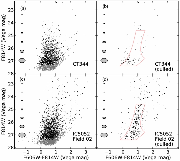
Figure 4. CMD of detections in an "empty" field dominated by unresolved background galaxies (CT344; panels a and b) and a sparse halo field (IC5052-Field 02; panels c and d). In panels (a) and (c), all detections in the respective fields with an error flag less than or equal to 2 and an object of type 1 (i.e., good detections) are plotted. The majority of these points are unresolved background galaxies which cannot easily be differentiated from stellar sources in ground-based photometry. Points in gray are those detections with an S/N >3.5, points in black are with an S/N >5.0. These two S/N regimes are plotted to emphasize the importance of culling by S/N. Shaded ellipses indicate the average 1σ error in F814W magnitude and color as calculated by dolphot at the indicated F814W magnitude. In panels (b) and (d), the same data points for the empty field and halo field, respectively, are shown using the sparse field selection criteria listed in Section 4.2. The region containing the recovered RGB stars in panel (d) is outlined and is repeated in panel (b) as a visual guide to differentiate the fields. Note that many of the detections in panel (d) brighter than 23.5 mag are likely foreground stars as IC 5052 is much closer to the galactic plane than the CT 344 field.
Download figure:
Standard image High-resolution imageTo optimize these selection criteria, we pass them to a routine that searches for improved solutions over a limited parameter space using a downhill simplex method. This was achieved by first populating all the "empty" archival fields listed in Table 3 with approximately 350,000 artificial stars. The distribution of these artificial stars was chosen to approximate the magnitude and color of the real detections in NGC 2403; they thus act as proxies for the true stars we wish to recover in our observations. The code then varied the parameters of the selection criteria to minimize the number of spurious detections in the "empty" fields, while maximizing the number of artificial stars recovered (see the Appendix for further details). The final selection criteria adopted for selecting stars in sparse fields are


where each parameter is a diagnostic of the stellar photometry output from dolphot. Additionally, to select only the most likely candidates, we use the detections for which dolphot reports an object of type 1 (i.e., a clean point source) and an error flag of 2 or less (not enough bad or saturated pixels to compromise the fit). We use the same selection criteria for crowded fields with the exception of the crowding cut, which we remove completely in uncrowded fields (see the Appendix).
After culling the data, some unresolved background galaxies inevitably remain (as shown for the CT344 archival field in panel (b) of Figure 4). However, the number of remaining contaminants is significantly fewer than the number of stars in the sparsest GHOSTS fields (e.g., panel (d) of Figure 4). To further quantify the effects of these contaminants, the surface density of false detections across all the "empty" fields in Table 3 is plotted as a function of F814W magnitude in Figure 5. Exposure time is found to have little effect on the distribution, other than varying the depth of the CMDs. Hence, at densities greater than 2.5 × 10⁻⁴ detections per mag per arcsec2, the trend across all the contaminant fields is a clear power law of log (dN/dF814W) =0.65 × F814W-19.0. This decreases to 0.62 × F814W-19.1 after culling the data with the crowded field selection criteria, and further flattens to 0.43 × F814W-14.4 after using the sparse field selection criteria.

Figure 5. Surface density of sources as a function of F814W magnitude. Red triangles in panel (a) indicate the contaminants combined from all the "empty" fields listed in Table 3. The lightest symbols plot all detections from dolphot with an S/N >5, an object type of 1 and an error flag ⩽2 (i.e., a good detection). Mid and dark tones are the same detections but are, respectively, culled with the crowded- and sparse-field selection criteria listed in Section 4.2. Dashed red lines denote extrapolated trends to fainter magnitudes with power laws plotted at densities greater than 2.5 × 10⁻⁴ detections per mag per arcsec2 of log (dN/dF814W) = 0.65 × F814W-19.0 for the lightest points, 0.62 × F814W-19.1, for the mid-tone (crowded-field selection criteria) points and 0.43 × F814W-14.4 for the darkest (sparse-field selection criteria) points. These dashed lines are repeated in panels (b) through (d) where the number of stars identified by dolphot in three different fields are also plotted. A sparse halo field in NGC 2403, the closest galaxy in the sample, is shown in panel (b). The black dot-dashed line indicates the location of the TRGB. The lightest points are all dolphot detections with S/N > 5 and an object type of 1, while darker symbols plot detections after culling with the sparse-field selection criteria. Panel (c) plots the deepest field in the sample from NGC 3031. The darker points this time are culled using the more lenient crowded-field selection criteria, both for the number of stars (dark filled circles) and number of contaminants (dark dashed lines). The red clump is a noticeable overdensity at F814W ∼27.7 mag. Panel (d) repeats the analysis for a sparse field in our second most distant galaxy: NGC 7814. The importance of accounting for background contamination is particularly evident in this panel. Before culling, the number of contaminants (light dashed lines) is comparable to the number of detected stars (light filled circles). After culling (dark dashed lines and dark circles), there is more than an order of magnitude difference at the TRGB.
Download figure:
Standard image High-resolution imageThese remaining spurious detections will limit the equivalent surface brightness that can be reached using resolved star counts. Specifically, the overall uncertainty on the measured stellar density will be a combination of the random Poisson error on the expected count rate of contaminants and halo stars, as well as a systematic uncertainty on the level of contamination. The systematic uncertainty on the expected mean level of contamination will remain the same for all binning prescriptions, but both Poisson noise terms will increase for decreasing bin sizes.
To illustrate the impact of these errors on surface brightness measurements, we calculate the S/N for detections in NGC 4565 (Figure 2). We restrict our analysis to contaminants with the same color as the RGB stars, assuming a distance modulus for NGC 4565 of 30.4. By integrating the contaminant luminosity function, we predict a total of 64.1 ± 8 (random) ± 7.7 (systematic) contaminants in a typical bin size of 80 arcsec−2. The systematic uncertainty is principally due to the uncertainty in the slope of the number of contaminants per magnitude. After culling by the sparse-field selection criteria, the expected number of contaminants decreases to 2.7 ± 1.6 (random) ± 1 (systematic). The overall noise before culling will thus be  , where N is the number of actual halo stars detected. Hence for an S/N greater than 10, we require 256 stars (noise =17.9 random +7.7 systematic). For NGC 4565, this equates to an equivalent surface brightness limit of I = 28.2 mag arcsec−2 (V ∼ 29.2 mag arcsec−2, converted using the typical RGB color measured in this survey). This limit improves substantially after culling, after which we only need 121 stars to reach the same S/N (noise =11.1 random +1 systematic). This number of stars equates to I = 29.0 mag arcsec−2 (V ∼ 30.0 mag arcsec−2), almost a magnitude fainter.
For ground-based observations, seeing limits the resolvable PSF to ∼04. Thus, the majority of contaminants removed by these selection culls will be indistinguishable from stars in ground-based images. This limits these observations to much higher equivalent surface brightnesses (e.g., Mouhcine et al. 2010; Bailin et al. 2011). Using the previous example, such observations would require over 960 stars in the same size bin to reach the same S/N, as the contaminants themselves now comprise the majority of noise. This equates to a surface brightness limit of I ∼ 27 mag arcsec−2, over 2 mag brighter.
5. COLOR–MAGNITUDE DIAGRAMS
As well as reaching low equivalent surface brightnesses, a key advantage to using resolved stellar populations over integrated light studies is the ability to differentiate the components of a galaxy by age and metallicity. Figure 6 highlights the distinct features observed in our CMDs, shown here for one of the outer fields of NGC 2403. The ages of these distinct regions depend on the star formation history (SFH) of the system. However, we can assign approximate age ranges by assuming a constant rate of formation (e.g., Figure 4 of Seth et al. 2005b). These ages, together with a description of the stellar populations that contribute to each region, are as follows.
- Main Sequence (MS): <300 Myr—these bluer stars are actively fusing hydrogen to helium in their cores. Their position on the sequence is primarily dictated by their mass which also determines their time on the sequence. Brighter stars toward the tip of the sequence are typically less than 100 Myr old.
- Red and Blue Helium-burning branches (RHeB and BHeB): 25–600 Myr—these massive, intermediate-age stars burn helium in their cores. During this phase, some of the red stars may quickly evolve to the blue sequence before eventually returning to the right of the CMD leading to blue loops. The rapid migration between states leads to the two distinct populations seen here. The specific color of the sequences, and so their separation, is metallicity dependent.
- Asymptotic Giant Branch (AGB): 1–3 Gyr—although the bulk of the helium-shell burning stars in this short-lived phase are 1–3 Gyr old, they will generally be at least 0.3 Gyr in age and possibly as old as 10 Gyr. However, the stars forming the observed tail to redder colors are mainly carbon stars, which are at most 3–5 Gyr old. Part of the AGB sequence overlaps with the RGB. However, the brighter AGB stars observed in the region identified here are most likely thermally pulsing AGB stars. In this state, the stars cycle between explosive burning of a helium shell and fusion of a hydrogen shell.
- Red Giant Branch (RGB): 8–12 Gyr—this region defines the oldest stars in the CMD and is principally composed of RGB stars undergoing shell hydrogen burning. Typically the RGB sequence is dominated by stars formed in the last significant starburst event, however RGB stars are always older than 1 Gyr. Metallicity strongly influences the position of the RGB stars in the CMD with higher metallicities leading to redder stars at a given magnitude. However, all RGB sequences with [Fe/H] <−0.7 reach approximately the same maximum magnitude at the TRGB.

Figure 6. Color–magnitude diagram for Field 02 of NGC 2403, which reaches three magnitudes below the TRGB (dashed red line), is presented in panel (a). At densities greater than 50 stars in a 0.1 × 0.1 mag bin in F814W and color, the data is plotted as a Hess diagram with contours at 100, 200, 350, and 500 stars per 0.01 mag2. Panel (b) identifies the key features of the CMD. These are the main sequence (MS), red giant branch (RGB), asymptotic giant branch (AGB), and red and blue helium-burning sequences (RHeB and BHeB). Also overlaid on panel (a) are a series of lines denoting the color distribution of single age populations of stars (= 10 Gyr, approximately corresponding to the RGB) for different metallicities taken from the Dartmouth Stellar Evolution Database (Dotter et al. 2008). In this case, the metallicity of the RGB sequence is approximately [Fe/H] = −1.2. The plotted stars have been filtered according to the crowded-field selection criteria described in Section 4.2.
Download figure:
Standard image High-resolution imageThe younger populations are most evident in the fields that lie on the galaxy disks, while the halo fields (and late-type bulge systems) predominantly show older stars. The color and slope of the RGB is sensitive to metallicity, as illustrated by the colored lines in panel (a) of Figure 6. Specifically, as the metallicity increases the RGB branch becomes redder and fainter.
The color of the RGB stars just below the well-defined TRGB can thus be used to estimate metallicity (e.g., Da Costa & Armandroff 1990; Bellazzini et al. 2001). There is some degeneracy with age using this technique. Worthey (1994) finds that stellar population models which differ according to Δage/ΔZ ∼ 3/2 are nearly indistinguishable. Using isochrones from the Dartmouth Stellar Evolution Database (Dotter et al. 2008), decreasing the age of a [Fe/H] = -1.0 RGB population from 10 to 3.33 Gyr shifts the color at half a magnitude below the TRGB by −0.11 mag. In comparison, decreasing the metallicity of the same 10 Gyr population by Δ[Fe/H] = log 2 shifts the color at the same magnitude by −0.16 mag. However, as this effect is not linear with age, the inferred metallicities can be underestimated when a range of stellar ages are present. Specifically, younger stars, which evolve quicker in color and form the bulk of the RGB track, are bluer than models based on globular clusters or 10 Gyr isochrones suggest. Hence metallicities inferred from colors should be treated as lower limits. For more accurate metallicities, a full SFH analysis is recommended. Despite these effects, our limited coverage of the top few magnitudes of the CMD still allows for better age/metallicity resolution than is currently possible with integrated light studies.
Figures 7–20 plot the field locations and CMDs for all the GHOSTS fields, including the reprocessed archival fields, which can vary significantly in exposure depth. Hess density diagrams are used when the number of stars is greater than 30 stars in a 0.1 × 0.1 mag bin in F814W and color, and are plotted with contours every 100, 200, 350, 500, 750, 1000, and 1500 stars per 0.01 mag2. Photometric errors, as reported by dolphot and averaged over the stars in the given magnitude bins, are indicated by ellipses. For each CMD the best-fit TRGB for the entire galaxy (described in Section 6) is marked by a red dot-dashed line, while a solid red line denotes the TRGB measurement for that specific field. Arrows in the upper right of each CMD indicate the direction of the reddening vector, and 20% completeness limits, as determined from the artificial star tests, are indicated with blue dashed lines.
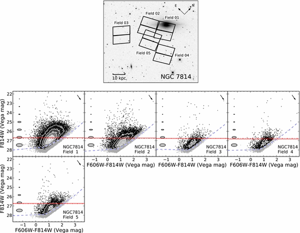
Figure 7. Fields in NGC 7814. The upper panel marks the field locations with the corresponding CMDs plotted below. The photometry is culled using the crowded-field selection criteria listed in Section 4.2. Points in gray are plotted with the same selection criteria but a lower S/N cut of 3.0 to illustrate the spread of the data at fainter magnitudes. At densities greater than 30 stars in a 0.1 × 0.1 mag bin in F814W and color, the data are plotted as a Hess diagram with contours at 100, 200, 350, 500, 750, 1000, and 1500 stars per 0.01 mag2. Shaded ellipses indicate the average 1σ uncertainties in the photometry as calculated by dolphot for the given F814W magnitude. The red dot-dashed line indicates the best TRGB magnitude for the entire galaxy (using the average RGB color) as reported in Section 6, while solid lines indicate the TRGB measurement for the individual field. Unless otherwise stated in the following figure captions, only TRGB detections denoted by solid lines are used in the overall TRGB measurement. Blue dashed lines denote the 20% completeness limit, as determined from artificial star tests. The direction of reddening due to foreground Galactic extinction is indicated by the arrow in the top right of each CMD. The data are corrected for this effect, which is typically a few hundredths of a magnitude in F814W and color.
Download figure:
Standard image High-resolution image
Figure 8. Fields and CMDs of NGC 0253, as described in Figure 7.
Download figure:
Standard image High-resolution image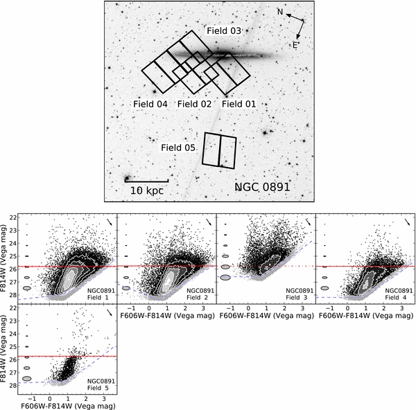
Figure 9. Fields and CMDs of NGC 0891, as described in Figure 7.
Download figure:
Standard image High-resolution image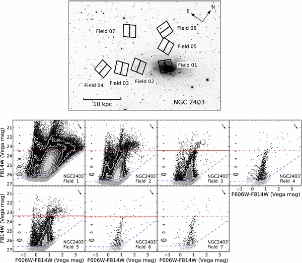
Figure 10. Fields and CMDs of NGC 2403, as described in Figure 7. The distribution of stars near the TRGB of Field 04 led to substantial uncertainty in assessing the TRGB magnitude of this field. Hence no detection is reported here.
Download figure:
Standard image High-resolution image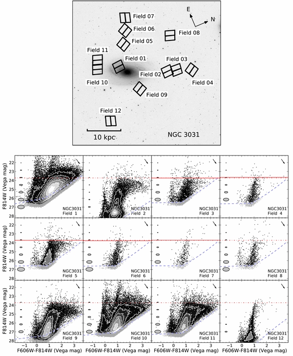
Figure 11. Fields and CMDs of NGC 3031 (M 81), as described in Figure 7.
Download figure:
Standard image High-resolution image
Figure 12. Fields and CMDs of NGC 4244, as described in Figure 7.
Download figure:
Standard image High-resolution image
Figure 13. Fields and CMDs of NGC 4565, as described in Figure 7.
Download figure:
Standard image High-resolution image
Figure 14. Fields and CMDs of NGC 4631, as described in Figure 7.
Download figure:
Standard image High-resolution image
Figure 15. Fields and CMDs of NGC 4736 (M 94), as described in Figure 7.
Download figure:
Standard image High-resolution image
Figure 16. Fields and CMDs of NGC 5023, as described in Figure 7.
Download figure:
Standard image High-resolution image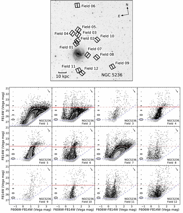
Figure 17. Fields and CMDs of NGC 5236 (M 83), as described in Figure 7. Note that Field 06 covers the companion dwarf galaxy UGCA 365, and that the CMD and associated TRGB detection is predominantly based on this system. Similarly, Fields 04 and 05 both lie on a significant stellar stream with a potentially different TRGB magnitude. Hence these three fields are not used in the averaged NGC 5236 distance measurement.
Download figure:
Standard image High-resolution image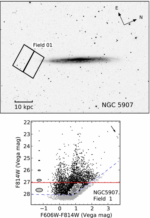
Figure 18. Fields and CMDs of NGC 5907, as described in Figure 7.
Download figure:
Standard image High-resolution image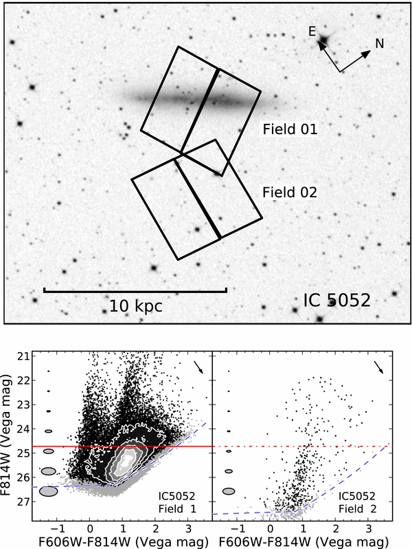
Figure 19. Fields and CMDs of IC 5052, as described in Figure 7.
Download figure:
Standard image High-resolution image
Figure 20. Fields and CMDs of NGC 7793, as described in Figure 7.
Download figure:
Standard image High-resolution image
6. TRGB DISTANCES
Stars evolving along the RGB sequence undergo a helium flash when the electron-degenerate helium core reaches a certain pressure and temperature. At this point, a rapid runaway fusion of helium is triggered that lasts until the degeneracy is removed (e.g., see Dearborn et al. 2006). As this process occurs at a constant critical mass, the maximum luminosity of the RGB sequence is theoretically well defined, particularly in the I band where the bolometric luminosity peaks (Lee et al. 1993; Salaris & Cassisi 1997; Salaris et al. 2002). For low-metallicity stars ([Fe/H] < -0.7), this limiting magnitude is known to be independent of age and only weakly dependent on metallicity. However, as the color of the stars at the TRGB can be used to measure their metallicity, this degeneracy can generally be accounted for. Although note that the precise color of the TRGB is partially dependent on the age and alpha abundance of the underlying population. Using the Da Costa & Armandroff (1990) sample of [Fe/H] < -0.7 globular clusters, Bellazzini et al. (2001) found that

where the metallicity is calculated on the Zinn & West (1984) scale. By inverting this relation and converting it to the Carretta & Gratton (1997) scale, Rizzi et al. (2007) have calculated the metallicity of HST-observed stars in several nearby galaxies. They subsequently used these values to infer the absolute magnitude of the horizontal branch (HB) stars, which is dependent on metallicity, for each system. Thus, by measuring the apparent magnitude of the TRGB relative to the HB stars, they were able to calibrate the following TRGB absolute magnitudes as functions of color of the TRGB:

or

By propagating the errors through this procedure, Rizzi et al. (2007) place an uncertainty of 0.02 mag on these calibrations.
To measure the apparent magnitude of the TRGB, we followed the same method employed by Seth et al. (2005a). Specifically, we used the logarithmic edge-detection algorithm defined in Méndez et al. (2002) on stars selected with a color cut to remove both MS and redder AGB stars. This cut was typically set at 0.3 < F606W-F814W < 1.6 but for fields with significant helium-burning sequences the range was shifted to redder colors (>1.0 mag). These intermediate-age stars are typically confined to the galaxy disks, but for a few systems, notably NGC 2403 and NGC 5236 (see Figures 10 and 17), they can be far removed from the galaxy center.
Generally, we only report TRGB measurements for fields that do not cover the main galaxy disk. This further minimizes contamination from younger stars and reduces the effects of internal extinction and crowding. However, for systems with only one field, or for galaxies that are sufficiently distant to easily discriminate the disk and halo populations in the same field, we still measured the TRGB. For these fields, we excluded the stars in regions of high surface brightness by using the galaxy masks produced in Section 3.2. Additionally, we only included fields with enough stars for convergence in the detection. Typically, this required at least 10 stars within the color cut and within 0.25 mag of the TRGB.
Although we measure colors of the RGB both at the TRGB and at MI = −3.5 (for comparison with Seth et al. 2005a), we do not infer metallicities. For significantly metal-poor stars, such as halo stars, the metallicities calculated from RGB colors may carry substantial uncertainties. We thus leave detailed metallicity calculations using analyses of full SFHs to future work.
Random errors in the TRGB detections were assessed by reprocessing 500 Monte Carlo resamples of the stellar magnitudes with replacement. At the TRGB magnitude, these random errors dominate the stellar photometric errors reported by dolphot. Hence an uncertainty in the TRGB magnitude was assigned by fitting a Gaussian to the distribution of the resamples. Further details of each TRGB detection and measurement are available on the GHOSTS Web site.16
Table 4 presents the results of the best TRGB detection for the measured fields together with the RGB color measurements and the associated distance modulus using the absolute magnitude defined in Equation (6). The error quoted on the distance modulus incorporates both the error in the TRGB detection and the error in the measurement of the color at the TRGB. Overall, some variation in the TRGB magnitude is seen between fields of the same galaxy. This could be due to shifts in the age and metallicity of the populations or increased reddening in the fields lying closer to the host galaxy. However, these variations are typically within the errors calculated from the Monte Carlo resamples.
Table 4. TRGB Results
| Galaxy | Field | No. of Tip | F814WTRGB | ITRGB | (F606W–F814W)TRGB | (V−I)TRGB | (V−I)−3.5 | m − MTRGB |
|---|---|---|---|---|---|---|---|---|
| Stars | (VEGAmag) | (Johnson) | (VEGAmag) | (Johnson) | (Johnson) | (mag) | ||
| (1) | (2) | (3) | (4) | (5) | (6) | (7) | (8) | (9) |
| NGC 7814 | 01 | 3366 | 26.69 ± 0.03 | 26.66 ± 0.03 | 1.27 ± 0.28 | 1.68 ± 0.36 | 1.30 ± 0.27 | 30.74 ± 0.08 |
| 02 | 1806 | 26.72 ± 0.03 | 26.71 ± 0.03 | 1.35 ± 0.30 | 1.78 ± 0.38 | 1.40 ± 0.24 | 30.76 ± 0.09 | |
| 03 | 286 | 26.76 ± 0.03 | 26.75 ± 0.03 | 1.20 ± 0.21 | 1.57 ± 0.28 | 1.35 ± 0.28 | 30.83 ± 0.08 | |
| 04 | 334 | 26.82 ± 0.04 | 26.79 ± 0.04 | 1.21 ± 0.22 | 1.61 ± 0.29 | 1.30 ± 0.25 | 30.88 ± 0.09 | |
| 05 | 881 | 26.73 ± 0.03 | 26.72 ± 0.03 | 1.31 ± 0.26 | 1.72 ± 0.32 | 1.46 ± 0.26 | 30.77 ± 0.08 | |
| NGC 0253 | 06 | 138 | 23.61 ± 0.02 | 23.60 ± 0.02 | 1.17 ± 0.14 | 1.54 ± 0.17 | 1.51 ± 0.23 | 27.68 ± 0.05 |
| 07 | 63 | 23.67 ± 0.02 | 23.66 ± 0.02 | 1.22 ± 0.19 | 1.60 ± 0.23 | 1.53 ± 0.28 | 27.73 ± 0.06 | |
| 08 | 90 | 23.61 ± 0.04 | 23.67 ± 0.04 | 1.30 ± 0.24 | 1.73 ± 0.29 | 1.57 ± 0.29 | 27.66 ± 0.09 | |
| 09 | 228 | 23.66 ± 0.03 | 23.65 ± 0.03 | 1.25 ± 0.19 | 1.64 ± 0.23 | 1.60 ± 0.26 | 27.72 ± 0.06 | |
| 10 | 563 | 23.69 ± 0.03 | 23.68 ± 0.03 | 1.38 ± 0.25 | 1.76 ± 0.28 | 1.66 ± 0.32 | 27.72 ± 0.08 | |
| NGC 0891 | 01 | 2411 | 25.80 ± 0.04 | 25.78 ± 0.04 | 1.39 ± 0.29 | 1.82 ± 0.36 | 1.64 ± 0.30 | 29.83 ± 0.10 |
| 02 | 1255 | 25.75 ± 0.03 | 25.73 ± 0.03 | 1.39 ± 0.29 | 1.81 ± 0.37 | 1.67 ± 0.31 | 29.78 ± 0.09 | |
| 04 | 381 | 25.78 ± 0.03 | 25.76 ± 0.03 | 1.32 ± 0.23 | 1.73 ± 0.29 | 1.62 ± 0.28 | 29.82 ± 0.08 | |
| 05 | 78 | 25.73 ± 0.04 | 25.71 ± 0.04 | 1.27 ± 0.17 | 1.67 ± 0.20 | 1.46 ± 0.21 | 29.78 ± 0.07 | |
| NGC 2403 | 03 | 98 | 23.43 ± 0.02 | 23.42 ± 0.02 | 1.13 ± 0.11 | 1.49 ± 0.14 | 1.33 ± 0.12 | 27.51 ± 0.05 |
| 05 | 117 | 23.38 ± 0.01 | 23.37 ± 0.01 | 1.19 ± 0.12 | 1.56 ± 0.14 | 1.38 ± 0.13 | 27.45 ± 0.04 | |
| 06 | 12 | 23.49 ± 0.02 | 23.47 ± 0.02 | 1.11 ± 0.08 | 1.51 ± 0.11 | 1.38 ± 0.25 | 27.57 ± 0.04 | |
| NGC 3031 | 03 | 37 | 23.73 ± 0.02 | 23.71 ± 0.02 | 1.20 ± 0.22 | 1.55 ± 0.26 | 1.56 ± 0.37 | 27.80 ± 0.07 |
| 04 | 13 | 23.66 ± 0.02 | 23.64 ± 0.02 | 1.12 ± 0.12 | 1.45 ± 0.16 | 1.37 ± 0.06 | 27.74 ± 0.04 | |
| 05 | 80 | 23.72 ± 0.04 | 23.70 ± 0.04 | 1.26 ± 0.21 | 1.65 ± 0.26 | 1.60 ± 0.29 | 27.77 ± 0.08 | |
| 06 | 22 | 23.77 ± 0.02 | 23.75 ± 0.02 | 1.05 ± 0.09 | 1.40 ± 0.17 | 1.39 ± 0.17 | 27.87 ± 0.04 | |
| 07 | 10 | 23.70 ± 0.02 | 23.68 ± 0.02 | 1.09 ± 0.07 | 1.50 ± 0.14 | 1.45 ± 0.47 | 27.79 ± 0.04 | |
| NGC 4244 | 03 | 236 | 24.24 ± 0.02 | 24.23 ± 0.02 | 1.04 ± 0.09 | 1.37 ± 0.12 | 1.24 ± 0.15 | 28.34 ± 0.04 |
| 06 | 43 | 24.02 ± 0.02 | 24.01 ± 0.02 | 1.15 ± 0.12 | 1.52 ± 0.17 | 1.39 ± 0.09 | 28.10 ± 0.05 | |
| 08 | 137 | 24.10 ± 0.03 | 24.08 ± 0.03 | 1.07 ± 0.11 | 1.41 ± 0.15 | 1.29 ± 0.16 | 28.19 ± 0.05 | |
| NGC 4565 | 01 | 1559 | 26.33 ± 0.02 | 26.32 ± 0.02 | 1.23 ± 0.21 | 1.62 ± 0.27 | 1.50 ± 0.30 | 30.39 ± 0.02 |
| 02 | 1220 | 26.34 ± 0.02 | 26.33 ± 0.02 | 1.31 ± 0.22 | 1.71 ± 0.27 | 1.58 ± 0.30 | 30.38 ± 0.02 | |
| 03 | 104 | 26.29 ± 0.03 | 26.28 ± 0.03 | 1.20 ± 0.21 | 1.58 ± 0.27 | 1.47 ± 0.24 | 30.36 ± 0.07 | |
| NGC 4631 | 01 | 1942 | 25.26 ± 0.03 | 25.25 ± 0.03 | 1.27 ± 0.25 | 1.67 ± 0.31 | 1.41 ± 0.26 | 29.31 ± 0.08 |
| 02 | 2338 | 25.31 ± 0.02 | 25.30 ± 0.02 | 1.21 ± 0.23 | 1.60 ± 0.29 | 1.43 ± 0.31 | 29.37 ± 0.03 | |
| NGC 4736 | 02 | 452 | 24.25 ± 0.03 | 24.24 ± 0.03 | 1.93 ± 0.49 | 2.50 ± 0.57 | 2.05 ± 0.43 | 28.17 ± 0.13 |
| 03 | 109 | 24.18 ± 0.04 | 24.17 ± 0.04 | 1.88 ± 0.52 | 2.40 ± 0.60 | 2.05 ± 0.57 | 28.11 ± 0.14 | |
| NGC 5023 | 01 | 258 | 24.98 ± 0.04 | 24.97 ± 0.04 | 1.13 ± 0.17 | 1.50 ± 0.22 | 1.29 ± 0.23 | 29.06 ± 0.07 |
| NGC 5236 | 02 | 185 | 24.40 ± 0.03 | 24.38 ± 0.03 | 1.50 ± 0.53 | 1.98 ± 0.66 | 2.11 ± 0.65 | 28.41 ± 0.13 |
| 04 | 69 | 24.32 ± 0.04 | 24.30 ± 0.04 | 1.27 ± 0.24 | 1.65 ± 0.33 | 1.45 ± 0.17 | 28.37 ± 0.08 | |
| 05 | 247 | 24.35 ± 0.03 | 24.33 ± 0.03 | 1.30 ± 0.17 | 1.70 ± 0.21 | 1.48 ± 0.17 | 28.39 ± 0.06 | |
| 06 | 404 | 24.48 ± 0.03 | 24.46 ± 0.03 | 1.04 ± 0.08 | 1.38 ± 0.11 | 1.25 ± 0.12 | 28.58 ± 0.05 | |
| 10 | 31 | 24.34 ± 0.04 | 24.32 ± 0.04 | 1.13 ± 0.15 | 1.45 ± 0.20 | 1.31 ± 0.10 | 28.42 ± 0.07 | |
| NGC 5907 | 01 | 325 | 27.05 ± 0.04 | 27.04 ± 0.04 | 1.14 ± 0.29 | 1.51 ± 0.36 | 1.26 ± 0.31 | 31.13 ± 0.10 |
| IC 5052 | 01 | 842 | 24.72 ± 0.05 | 24.70 ± 0.05 | 1.34 ± 0.22 | 1.76 ± 0.28 | 1.57 ± 0.25 | 28.76 ± 0.10 |
| NGC 7793 | 01 | 120 | 23.79 ± 0.02 | 23.78 ± 0.02 | 1.21 ± 0.20 | 1.60 ± 0.25 | 1.46 ± 0.15 | 27.85 ± 0.06 |
| 02 | 21 | 23.86 ± 0.03 | 23.84 ± 0.03 | 1.09 ± 0.09 | 1.46 ± 0.16 | 1.32 ± 0.17 | 27.95 ± 0.05 | |
| 03 | 36 | 23.72 ± 0.04 | 23.70 ± 0.04 | 1.14 ± 0.10 | 1.51 ± 0.12 | 1.36 ± 0.13 | 27.80 ± 0.06 |
Notes. Detections of the TRGB for fields with enough stars for convergence of the Monte Carlo resamples that are not heavily contaminated by young stars. Columns are: (1) galaxy identifier; (2) field number; (3) number of stars within the color cut and within 0.25 mag of the TRGB; (4) and (5) F606W and I-band magnitude of the TRGB. Quoted errors are the spread in 500 Monte Carlo realizations of the data; (7) and (8) mean V − I colors at the TRGB and at an absolute magnitude of −3.5. Errors are the width of the Gaussian fitted across the distributions; (9) distance modulus calculated using the detection in Column 4, the color in Column 6 and Equation (6). The reported error incorporates the errors both in the TRGB magnitude and the color. Also note that the TRGB detection reported for NGC 5236-Field 06 is that of the companion dwarf galaxy UGCA 365. The measurement is reported here but not used for the average distance modulus computed for NGC 5236 in Table 5.
Download table as: ASCIITypeset image
A few notable features are evident in the TRGB detections. First, although stars are observable below the TRGB in NGC 0891-Field 03 and NGC 4565-Field 04 as required by the survey constraints, the observations are too shallow for a reliable TRGB detection after applying the selection criteria. Both these fields were observed in the Cycle 12 SNAPshot program, which was principally designed to study the dust lanes across the bright central regions of these systems. Second, the TRGBs in Fields 04 and 05 of NGC 5236 are slightly brighter than the detection in the inner field. This can be attributed to the stellar stream that passes through these fields, which also produces a distinct AGB population not seen in the other halo fields. The brighter TRGB suggests that the stream may lie slightly in the foreground of the host galaxy. This feature will be discussed further in a future paper. Lastly, although NGC 5236-Field 09 lies on the bright spiral galaxy MCG-05-32-042, the system is too distant to resolve individual stars (although globular clusters in this system may be mistaken for NGC 5236 stars). However, NGC 5236-Field 06 covers the dwarf galaxy UGCA 365, which lies in the vicinity of NGC 5236 and so accounts for the bulk of the stars in this field. Using the distance modulus in Table 4, we infer a distance of 5.2 ± 0.1 Mpc for this system.
Table 5 presents an overall distance modulus for each galaxy together with distance moduli taken from the literature. These include measurements inferred from Cepheid variables, SBFs, planetary nebula luminosity functions (PNLFs), and TRGB measurements. For systems with detections in more than one field, we compute the mean distance modulus. However, for NGC 5236 we do not include Fields 04 and 05, as they are dominated by a significant stellar stream as previously mentioned, nor do we include Field 06 as this covers the dwarf galaxy UGCA 365. For the overall uncertainty, the error for each field is combined in quadrature, and for systems with three or more measurements, this error is also combined in quadrature with an estimate of the standard deviation of the results. Overall, measurements from the literature agree favorably with the final galaxy TRGB distances measured here.
Table 5. Distance Moduli
| Galaxy | m − MTRGB | D | m − MCepheid | m − MSBF | m − MPNLF | m − MTRGB |
|---|---|---|---|---|---|---|
| (GHOSTS) | (GHOSTS) | |||||
| (mag) | (Mpc) | (mag) | (mag) | (mag) | (mag) | |
| (1) | (2) | (3) | (4) | (5) | (6) | (7) |
| NGC 7814 | 30.80 ± 0.10 | 14.4+0.7− 0.6 | ... | 30.44 ± 0.14(1) | ... | ... |
| NGC 0253 | 27.70 ± 0.07 | 3.5 ± 0.1 | ... | ... | 27.62 ± 0.26(2) | 27.7 ± 0.14(3) |
| NGC 0891 | 29.80 ± 0.09 | 9.1 ± 0.4 | ... | 29.61 ± 0.14(4) | 29.99 ± 0.13(5) | 29.82(6) |
| NGC 2403 | 27.51 ± 0.07 | 3.2 ± 0.1 | 27.43 ± 0.15(7) | ... | 27.65 ± 0.17(5) | 27.52 ± 0.08(3) |
| NGC 3031 | 27.79 ± 0.07 | 3.6 ± 0.1 | 27.80 ± 0.09(7) | 27.80 ± 0.26(1) | 27.70 ± 0.09(5) | 27.77 ± 0.04(3) |
| NGC 4244 | 28.21 ± 0.11 | 4.4 ± 0.2 | ... | ... | ... | 28.20 ± 0.03(8) |
| NGC 4565 | 30.38 ± 0.05 | 11.9+0.3− 0.2 | ... | 31.05 ± 0.17(1) | 30.08 ± 0.15(5) | ... |
| NGC 4631 | 29.34 ± 0.06 | 7.4 ± 0.2 | ... | ... | ... | 29.41 ± 0.04(8) |
| NGC 4736 | 28.14 ± 0.13 | 4.2 ± 0.3 | ... | 28.58 ± 0.18(4) | 28.21 ± 0.06(9) | 28.34 ± 0.29(10) |
| NGC 5023a | 29.06 ± 0.07 | 6.5 ± 0.2 | ... | ... | ... | 29.10 ± 0.03(8) |
| NGC 5236 | 28.41 ± 0.11 | 4.8 ± 0.2 | 28.32 ± 0.13(7) | ... | 28.43 ± 0.60(9) | ... |
| NGC 5907a | 31.13 ± 0.10 | 16.8+0.8− 0.7 | ... | ... | ... | ... |
| IC 5052a | 28.76 ± 0.10 | 5.6+0.3− 0.2 | ... | ... | ... | 28.90 ± 0.04(8) |
| NGC 7793 | 27.87 ± 0.08 | 3.7 ± 0.1 | ... | ... | ... | 27.96 ± 0.24(11) |
Notes. For galaxies in the GHOSTS sample with multiple fields, the averaged distance modulus is listed using the individual TRGB detections reported in Table 4. The uncertainties on these fields are combined in quadrature for each galaxy, and where three or more measurements exist this is also combined in quadrature with an estimate of the standard deviation of the results. The most recent literature measurements are also shown. These are based on Cepheid variables, surface brightness fluctuations (SBFs), planetary nebula luminosity functions (PNLFs), and TRGB methods. Note that, for comparison, the Extragalactic distance database (Tully et al. 2009) records a distance modulus of 30.64 ± 0.35 for NGC 5907 using the Tully–Fisher method. aTable 4 lists a TRGB detection for only one field in this galaxy. That measurement, along with the quoted errors, is repeated here. References. (1) Jensen et al. 2003; (2) Rekola et al. 2005; (3) Dalcanton et al. 2009; (4) Tonry et al. 2001; (5) Ciardullo et al. 2002; (6) Mould & Sakai 2008; (7) Saha et al. 2006; (8) Seth et al. 2005a; (9) Herrmann et al. 2008; (10) Karachentsev et al. 2003b; (11) Karachentsev et al. 2003a.
Download table as: ASCIITypeset image
Using the artificial star tests, we find that the median depth at 50% completeness across all the fields in this survey is 2.7 mag below the TRGB. However, only 67 of the 76 GHOSTS fields reach at least 20% completeness at depths of 1.5 mag below the TRGB.
7. DATA PRODUCTS
The data from the GHOSTS survey will be distributed as a "High-Level Science Product" on the MAST Web site.16 For each field, including those taken from the archive, the following will be released.
- 1.*.phot_sparse.gz: the raw photometry files output by dolphot using the parameters for sparsely populated fields (which are also listed in *sparse.param). Descriptions of the columns are given in the dolphot manual.17
- 2.*.phot_crowded.gz: similarly, the raw photometry files output by dolphot but using the parameters for crowded fields (which are also listed in *crowded.param).
- 3.*.stars.fits: the final filtered catalog of stars, listed separately for photometry using either the sparse or crowded field parameters together with the corresponding selection criteria from Section 4.2. The columns are X, Y (relative to the F814W drizzled image), RA, DEC, MAG1_ACS, MAG1_JC, MAG1_ERR, CHI1, SNR1, SHARP1, ROUND1, CROWD1, FLAG1, MAG2_ACS, MAG2_JC, MAG2_ERR, CHI2, SNR2, SHARP2, ROUND2, CROWD2, FLAG2, where "1" refers to the ACS filter listed under the header keyword "FILTER1" (typically F606W) and "2" refers to the "FILTER2" keyword (typically F814W). The *_ACS column lists the instrumental magnitudes recorded in VEGAMAG, and the *_JC column lists the corresponding Johnson–Cousins magnitudes, which are V for F606W and I for F814W. Subsequent columns are the dolphot parameters summarized in Section 3.3 with "FLAG" indicating the error flag. The header lists the zero-point corrections applied, together with additional data such as completeness at F606W–F814W = 0.75 (as computed from the artificial star tests) and the detected TRGB magnitude.
- 4.*.drz.fits: the final cleaned drizzled images, both in the F606W and F814W filters. The F814W image is used for coordinate references.
- 5.*.gal.fits: where applicable, the galaxy mask, which was used to exclude spurious detections of extended objects coincident with the host galaxy disk, and to exclude high-extinction regions when calculating the TRGB distance.
- 6.*.seg.fits: the segmentation mask, which identifies the extended objects in the drizzled image
- 7.*.se: the SExtractor catalog from which the above mask is constructed.
- 8.*.sky.fits: the background sky image computed by running the calcsky routine included in the dolphot package on the drizzled F814W image. This file is used for sky brightness in the artificial star tests.
- 9.*.artificial.fits: the three-dimensional probability distribution of recovering a star, computed separately for the sparse and crowded field culls, as a function of magnitude in the F814W filter, F814W–F606W color, and background sky brightness. Bins without sufficient coverage in the artificial star tests to compute a probability are set to zero.
Additionally, more diagnostic plots that display the results of the culls are presented on the GHOSTS Web site, together with further information regarding the TRGB detection for individual fields.
8. SUMMARY
We have presented an overview of the GHOSTS survey and described the reduction of the ACS/WFC F606W and F814W imaging in 14 nearby disk galaxies. Across the survey, we have reliably measured the photometry of some 3.1 million stars in 76 ACS fields. For each of these fields we have also generated a few million artificial stars, which reveal the median depth of the survey at 50% completeness to be 2.7 mag below the TRGB. The mean photometric error for all stars with an S/N >10 is ∼0.06 mag. By repeating our analysis on fields from the MAST archive that are free of resolvable stars, we find the principal contaminant in the survey to be unresolved background galaxies. In sparse fields, these sources lead to a larger error than can be attributed to the small number statistics of the RGB tracers. Hence, when equating RGB stellar densities to surface brightness, the background galaxies limit the measurable brightness. However, by specifying various selection criteria, which have subsequently been optimized by an automated routine, approximately 95% of the contaminants can be removed. For NGC 4565, this corresponds to an equivalent surface brightness limit of I ∼ 29 mag arcsec−2 (V ∼ 30 mag arcsec−2). Without the selection criteria, this limit is almost a magnitude brighter, and by simulating atmospheric seeing conditions, we expect the same limit for ground-based observations to be some two magnitudes brighter. We have used this culled photometry to measure the TRGB distances to all the galaxies in the survey. The uncertainties on these measurements ranges from only ∼2% to 7% of the total value.
This survey represents the largest sample of resolved stellar populations in the outskirts of disk galaxies to date. The combination of our observations with high-resolution N-body simulations will undoubtedly yield significant advances in the study of disk galaxy assembly and evolution.
Support for Proposal numbers 9765, 10523, and 10889 was provided by NASA through a grant from the Space Telescope Science Institute, which is operated by the Association of Universities for Research in Astronomy, Incorporated, under NASA contract NAS5-26555. Additionally, some of the data presented in this paper were obtained from the Multimission Archive at the Space Telescope Science Institute (MAST). Support for MAST for non-HST data is provided by the NASA Office of Space Science via grant NNX09AF08G and by other grants and contracts. This research has made use of the NASA/IPAC Extragalactic Database (NED) which is operated by the Jet Propulsion Laboratory, California Institute of Technology, under contract with the National Aeronautics and Space Administration. We acknowledge the usage of the HyperLeda database (http://leda.univ-lyon1.fr). This research has also made use of NASA's Astrophysics Data System Bibliographic Services. S.C. acknowledges the support of a Discovery Grant from the Natural Sciences and Engineering Research Council of Canada.
Facility: HST (ACS) - Hubble Space Telescope satellite
APPENDIX: AUTOMATED SELECTION CRITERIA DETERMINATION
As described in Section 4.2, we employed an automated routine to determine the best selection criteria for both our sparsely populated and our crowded fields. This code principally worked on the "empty" archival fields listed in Table 3, which should be free of resolvable stars outside of our own Galaxy. Any detection which dolphot recorded in these fields was thus spurious and was likely an unresolved background galaxy (given that the density of foreground Milky Way stars is low). These false detections needed to be reduced by employing a series of selection criteria. At the same time, these selection criteria must have minimal impact on the number of true stellar detections reported. To that end, we re-ran dolphot on the archival fields after populating them with ∼350,000 artificial stars, distributed to approximately recreate the CMD of NGC 2403-Field 02. Ideally, all of these artificial stars should be recovered by dolphot. The automated routine thus took both the spurious detections and the artificial star results together with a series of selection criteria as input. By employing a simple downhill-simplex optimization routine, the code then searched for improved solutions to the selection criteria. Specifically, the code maximized the figure of merit, F, defined by
where fa, i and fc, i are, respectively, the fraction of artificial stars and the fraction of contaminants (spurious detections in the empty fields) passed by the selection criteria in field i. After experimentation, the parameter α was set to 2 to achieve an optimal balance (i.e., passing ∼85% of the artificial stars and only ∼5% of the spurious detections). The first summation is over all the empty archival fields, while the second is over the fields: NGC 2403-Field 01, NGC 4244-Field 01, and NGC 4631-Field 01. These three GHOSTS fields, located on the central bulge of each galaxy, were included to ensure the optimized selection criteria were also suitable for use in fields with significant crowding. However, as GHOSTS is principally concerned with sparsely populated fields in the outskirts of galaxies, β, after further investigation, was set to 0.1 so as not to weigh these fields too heavily in the calculation. To avoid local minima, the code was executed several hundred times with different seed values. The final solution was the median value from all these runs.
We initially defined a number of selection criteria to pass through the optimization code, including those from the ANGST survey. These are listed in the upper half of Table 6, with the corresponding optimized values asterisked and listed in the lower half. The table also includes the fraction of artificial stars that were recovered in crowded fields (NGC 4631-Field 01, NGC 4244-Field 01, and NGC 2403-Field 01). Comparing the selection criteria labeled ANGST 1 and ANGST 2 clearly shows the impact of this crowding. Here, the difference in recovering artificial stars (our proxies for actual stellar detections) in the "empty" fields is only 6.6%. However, the more lax criteria pass almost three times as many spurious detections (32% cf. 11%). While this may seem disadvantageous, this same lax criterion also passes almost three times as many artificial stars in the crowded fields. As there are a few million such "real" stars in crowded fields, compared to only a few thousand contaminating objects, this lax criterion results in a much higher S/N.
Table 6. Photometry Culls
| ID | Crowding | Sharpness | Roundness | S/N | Artificial Star | Fraction of Spurious | Artificial Star |
|---|---|---|---|---|---|---|---|
| Recovery Fraction | Detections Passed | Recovery Fraction | |||||
| in "Empty" Fields | in "Empty" Fields | in Crowded Fields | |||||
| (mag) | (%) | (%) | (%) | ||||
| ANGST 1 | V + I < 0.1 | (V + I)2 ⩽ 0.075 | ... | V > 4, I > 4 | 86.1 | 11.4 | 18.8 |
| ANGST 2 | V + I < 0.6 | (V + I)2 ⩽ 0.075 | ... | V > 4, I > 4 | 92.7 | 32.3 | 52.5 |
| Cull 1 | V + I < 0.1 |  < 1.0, V + I > −0.05 < 1.0, V + I > −0.05 |
V + I < 4 | V > 4, I > 4 | 82.7 | 4.2 | 18.4 |
| Cull 2 | V + I < 0.1 | −0.05 > V + I < 1.4 | V + I < 4 | V > 4, I > 4 | 83.3 | 4.6 | 18.4 |
| Cull 3 | V + I < 0.1 | −0.05 > V + I < 1.4 | ... | V > 4, I > 4 | 83.3 | 4.6 | 18.4 |
| Cull 4 | ... | −0.05 > V + I < 1.4 | V + I < 4 | V > 4, I > 4 | 89.2 | 10.4 | 54.4 |
| Cull 5 | V + I < 0.1 | ... | V + I < 4 | V > 4, I > 4 | 86.3 | 20.0 | 18.8 |
| Cull 6 | ... | −0.05 > V + I < 1.4 | ... | V > 4, I > 4 | 89.2 | 10.7 | 55.3 |
| ANGST* | V + I < 0.09 | (V + I)2 ⩽ 0.04 | ... | V > 0.04, I > 0.04 | 86.2 | 11.0 | 17.2 |
| Cull 1* | V + I < 0.19 |  < 1.0, (V + I) > −0.5 < 1.0, (V + I) > −0.5 |
V + I < 3.31 | V > 4.7, I > 4.7 | 85.8 | 5.2 | 27.6 |
| Cull 2* | V + I < 0.19 | −0.06 > V + I < 1.46 | V + I < 1.50 | V > 4.2, I > 4.2 | 87.0 | 5.5 | 27.9 |
| Cull 3* (Sparse Field) | V + I < 0.16 | −0.06 > V + I < 1.30 | ... | V > 5.0, I > 5.0 | 85.3 | 5.0 | 24.3 |
| Cull 4* | ... | −0.04 > V + I < 1.39 | V + I < 2.94 | V > 5.8, I > 5.8 | 84.1 | 5.3 | 50.0 |
| Cull 5* | V + I < 0.07 | ... | V + I < 2.60 | V > 6.9, I > 6.9 | 77.8 | 8.6 | 14.0 |
| Cull 6* | ... | −0.04 > V + I < 1.35 | ... | V > 5.8, I > 5.8 | 84.1 | 5.3 | 51.1 |
| Cull 7 (Crowded Field) | ... | −0.06 > V + I < 1.30 | ... | V > 5.0, I > 5.0 | 87.7 | 8.3 | 55.7 |
Notes. The various selection criteria explored together with the corresponding recovery fraction. These fractions are listed for the ∼350,000 artificial stars generated in the "empty" fields of Table 3, the ∼20,000 spurious detections reported by dolphot in these fields, and the ∼180,000 artificial stars generated in the crowded fields NGC 2403-Field 01, NGC 4244-Field 01, and NGC 4631-Field 01. Culls in the top portion of the table are the initially defined criteria, which are subsequently passed through the optimization routine. The ANGST 1 cull lists the selection criteria used in Dalcanton et al. (2009), while ANGST 2 relaxes the crowding cull to ensure recovery of the star clusters in Gogarten et al. (2009). Asterisked culls in the second portion of the table are the equivalent culls after they have been passed through the optimization routine. The final Cull 7 simply repeats the optimized criteria from Cull 3* but omits the crowding cull. These two culls, i.e., 3 and 7, are adopted as the final culls for sparse and crowded fields, respectively. V and I are used as shorthand for the equivalent F606W and F814W dolphot parameters, e.g., a V in the Crowding column is the crowding parameter output by dolphot for the F606W filter. Note that all selection criteria additionally only select detections with a dolphot reported object type of 1 (i.e., a clean point source) and an error flag of 2 or less (not enough bad or saturated pixels to compromise the fit).
Download table as: ASCIITypeset image
The various selection criteria in Cull 1 were developed by comparing the distributions of the spurious detections and the true stellar detections in a variety of parameter spaces. However, as can be seen by comparing the recovery fractions of Cull 1 and Cull 2 (differences ∼1%), there is little to be gained by the complicated Cull 1 prescription. Hence, we focused on the simpler Culls 2–6, in order to explore the effects of selecting on the various dolphot diagnostic values. Immediately evident from the initial criteria is that the roundness parameter has little effect on improving the data quality (no change in the recovery fraction between Culls 2 and 3). Conversely, crowding and sharpness have the largest impact on discriminating true and spurious detections. Hence in sparsely populated fields, we adopt the optimized Cull 3* as our preferred selection criteria. Unfortunately, in crowded fields, such as those on the galaxy disk, culling by crowding removes a significant fraction of the detections (24% "real" stars remain using the crowding parameter compared to 56% without). For these fields we could adopt the equivalent Cull 6*. However, with this cull, and Culls 4* and 5*, the optimization routine attempts to compensate for the loss of the crowding or sharpness parameters by placing greater emphasis on the S/N cut. As S/N approximately correlates with magnitude, this results in significant loss of data at faint magnitudes. We thus instead use Cull 3*, but simply omit the crowding criteria for our crowded fields. This also allows for a more direct comparison between the two regimes. The effect of this new selection criteria is listed as Cull 7 in Table 6. Although the associated selection criteria pass more contaminants than Cull 6*, the increased number of artificial stars recovered in crowded fields more than compensates when this selection criterion is used on such fields.
Footnotes
- 12
- 13
- 14
http://www.stsci.edu/hst/acs/analysis/zeropoints—last modified 2010 November 17.
- 15
- 16
- 17