


ABSTRACT
We present Spitzer Space Telescope IRAC and MIPS observations of a 0.85 deg2 field including the Corona Australis (CrA) star-forming region. At a distance of 130 pc, CrA is one of the closest regions known to be actively forming stars, particularly within its embedded association, the Coronet. Using the Spitzer data, we identify 51 young stellar objects (YSOs) in CrA which include sources in the well-studied Coronet cluster as well as sources distributed throughout the molecular cloud. Twelve of the YSOs discussed are new candidates, one of which is located in the Coronet. Known YSOs retrieved from the literature are also added to the list, and a total of 116 candidate YSOs in CrA are compiled. Based on these YSO candidates, the star formation rate is computed to be 12 M☉ Myr−1, similar to that of the Lupus clouds. A clustering analysis was also performed, finding that the main cluster core, consisting of 68 members, is elongated (having an aspect ratio of 2.36), with a circular radius of 0.59 pc and mean surface density of 150 pc−2. In addition, we analyze outflows and jets in CrA by means of new CO and H2 data. We present 1.3 mm interferometric continuum observations made with the Submillimeter Array (SMA) covering R CrA, IRS 5, IRS 7, and IRAS 18595-3712 (IRAS 32). We also present multi-epoch H2 maps and detect jets and outflows, study their proper motions, and identify exciting sources. The Spitzer and ISAAC/VLT observations of IRAS 32 show a bipolar precessing jet, which drives a CO(2–1) outflow detected in the SMA observations. There is also clear evidence for a parsec-scale precessing outflow, which is east–west oriented and originates in the SMA 2 region and likely driven by SMA 2 or IRS 7A.
Export citation and abstract BibTeX RIS
1. INTRODUCTION
The Gould Belt Spitzer Legacy program is a GO-4 program designed to extend the earlier Spitzer Cores to Disks (c2d; Evans et al. 2003, 2009) program, thereby completing a census of star-forming regions within 500 pc. The Gould Belt is a band of stars and molecular clouds located within ∼20° of the Galactic Plane (Herschel 1847; Gould 1879). Although, at a declination of approximately −40°, Corona Australis (CrA) is not technically within the Gould Belt, it is discussed in this paper as part of the survey. We present an extensive study of the entire Corona Australis star-forming region, investigating the overall young population, its spatial distribution along the molecular cloud, and the young stellar object (YSO) outflows.
Rossano (1978) used star counts to create an extinction map, and identified five clouds in CrA, named clouds A–E, noting that CrA is highly elongated, oriented nearly east to west in the sky. Cloud A is in the west, and it is this cloud which corresponds to the R CrA/Coronet region. Large-scale CO mapping by Loren (1979) also shows this elongation, but their high spatial resolution observations of the velocity field indicated no velocity gradient. Loren (1979) interpreted this to mean that the elongation is not due to contraction along the rotational axis. However, Harju et al. (1993) argued that the Loren (1979) data were not sufficient, and suggest from their own C18O observations that the R CrA core is, in fact, a fragmented disk, explaining the observed elongation along the major axis. It is somewhat surprising that CrA is not associated with the Gould Belt, considering its close distance of 130 pc12; Mamajek & Feigelson (2001) argue that instead it formed as part of expanding Sco-Cen superbubbles, specifically Loop I, citing evidence from the Harju et al. (1993) millimeter observations, and radio observations from Cappa de Nicolau & Poppel (1991).
Studies from the literature have mainly focused on R CrA, the brightest star in the cluster, the Coronet region, and its population. The variability of the nebula surrounding the Herbig Ae star, R CrA, has been known since the early 1900s (Knox Shaw 1916; Reynolds 1916). Many years later, the two variable stars R CrA and T CrA were identified by Herbig (1960) to be young, and he then concluded that the associated stars should also be young. This prompted an interest in studying the R CrA region, and in 1973, the first major optical and infrared study of the main stars near R CrA was conducted, finding a total of 11 stars in the young stellar group: TY CrA, S CrA, T CrA, R CrA, DG CrA, VV CrA, KS-15, HR 7169, HR 7170, Anon 1, and Anon 2 (Knacke et al. 1973). The following year, IRS 1 was suggested by Strom et al. (1974) to be the driving source for the Herbig-Haro (HH) object, HH 100. Subsequent infrared observations were made by many groups (Glass & Penston 1975; Vrba et al. 1976a; Taylor & Storey 1984; Wilking et al. 1986) as well as Hα observations (Marraco & Rydgren 1981) and emission-line observations (Graham 1993). These were followed by early X-ray (Walter 1986; Koyama et al. 1996; Neuhäuser & Preibisch 1997; Walter et al. 1997; Patten 1998), radio (Brown 1987; Cappa de Nicolau & Poppel 1991), millimeter (Harju et al. 1993), and far-infrared studies (Wilking et al. 1992, who first mentioned IRAS 32).
Neuhäuser & Forbrich (2008) have recently reviewed the literature on the entire Corona Australis star-forming region, although many of the studies cover only a subset of the region which we include here as part of our Spitzer IRAC and MIPS study. The most relevant recent studies include: deep infrared observations (Wilking et al. 1997; Haas et al. 2008), millimeter and submillimeter observations (Chini et al. 2003; Groppi et al. 2004; Nutter et al. 2005) including Submillimeter Array (SMA) observations (Groppi et al. 2007), mid-infrared observations with the Infrared Space Observatory (ISO; Olofsson et al. 1999), and a series of papers focusing on Chandra X-ray studies of the region (Forbrich et al. 2006, 2007; Forbrich & Preibisch 2007). Finally, some spectroscopic work has been done to determine association memberships (Patten 1998; Nisini et al. 2005; Sicilia-Aguilar et al. 2008; Meyer & Wilking 2009).
The most massive stars in CrA are the Herbig Ae/Be stars, R CrA, and TY CrA. R CrA has a spectral type of A5 (Knacke et al. 1973; Marraco & Rydgren 1981) and is located at the tip of a cometary-shaped reflection nebula, NGC 6729. TY CrA, located ∼5' to the northwest of R CrA, is at least a quadruple system (Casey et al. 1995; Chauvin et al. 2003) where the primary has a spectral type of B8–B9 (Herbig & Kameswara Rao 1972; Knacke et al. 1973; Marraco & Rydgren 1981), and is associated with the reflection nebula NGC 6726/7. Located 1' south of TY CrA is HD 176386, which is also surrounded by reflection nebulosity from NGC 6727 (Knacke et al. 1973; Marraco & Rydgren 1981). HD 176386 is a binary system, first recognized as such by Wilking et al. (1997); HD 176386A/B is a visual pair separated by 3 7 with spectral types of A0V and K7, respectively (Meyer & Wilking 2009). Additionally, a little further from the Coronet (∼12' to the southwest of R CrA) lie two B8V stars, HR 7169 and HR 7170, which are discussed in more detail in Appendix A.11. Evidence for heating of the molecular cloud by these two B8 stars has been seen (Loren 1979), making it likely that there is a physical association and that they are therefore located at the same distance as R CrA (see further discussion in Neuhäuser et al. 2000).
CrA is also known to harbor many active YSOs with outflows. To date, 20 HH objects, including 48 different knots, have been discovered in the CrA star-forming region. Eight objects (HH 82, 96–101, 104) were detected in the 1970s and 1980s (Strom et al. 1974; Schwartz et al. 1984; Hartigan & Graham 1987; Reipurth & Graham 1988), while the remaining 12 objects were observed by Wang et al. (2004) in a large optical survey. The majority of the detected objects are located close to the Coronet and seem to be driven by YSOs inside it or in its outskirts. A few more HH objects are positioned close to HH100-IR (IRS 1), S CrA, VV CrA and IRAS 18595-3712 (IRAS 32), which seem to drive outflows as well. On the other hand, there are very few and sparse studies on H2 jets and outflows in CrA (see, e.g., Wilking et al. 1990; Gredel 1994; Davis et al. 1999; Caratti o Garatti et al. 2006). In these papers, the H2 counterparts of HH 99, 100, 101 and 104 were identified and studied, and a few new jets in the Coronet were detected (Caratti o Garatti et al. 2006). Davis et al. (2010) cataloged five molecular hydrogen objects (MHOs, MHO 2000–2004), but so far, an extensive H2 map of the region has not been made. Thus, a complete census of outflows and their driving sources is lacking.
We present Spitzer observations of a 0.85 deg2 region in the Corona Australis molecular cloud, identifying the Spitzer-selected YSOs distributed throughout the cloud as well as the outflows and their driving sources. This study includes infrared imaging of a much larger portion of the molecular cloud than many previous studies have included. In Section 2, we discuss the Spitzer observations and data reduction, including basic statistics for the sources detected, as well as the ancillary SMA observations, and H2 observations of outflows. In Section 3, we discuss methods used to select YSO candidates from color–magnitude diagrams constructed from the Spitzer data, as well as other methods of selection. We also discuss the addition of known YSOs and YSO candidates from the literature because they were not classified from Spitzer data due to saturation or other observational issues. The distribution of YSOs is discussed in Section 4. There we present an extinction map created from near-infrared and Spitzer data, an analysis of the spatial distribution of the YSOs in the cloud, and the clustering analysis performed using the YSO candidates in CrA. In Section 5, we present an analysis of the SMA observations. In Section 6, we present an analysis of the jets and outflows, the proper motions (P.M.s) of the H2 knots, and the driving sources for the outflows and jets seen in CrA. Finally, in Section 7, we discuss the overall cloud properties and how they compare with the other regions (c2d and Gould Belt) and summarize the results in Section 8.
2. OBSERVATIONS AND DATA REDUCTION
2.1. Spitzer IRAC and MIPS
Corona Australis was observed with the Spitzer Infrared Array Camera (IRAC; Fazio et al. 2004) at 3.6, 4.5, 5.8, and 8.0 μm and the Multiband Imaging Photometer for Spitzer (MIPS; Rieke et al. 2004) at 24, 70, and 160 μm as part of two guaranteed time observation (GTO) programs (PID 6, 30784; PI: Fazio) as well as the Gould Belt Legacy Survey (PID 30574; PI: Allen). Table 1 summarizes the program identification numbers, AOR identification numbers, and observation dates for all of the CrA data included in this paper. The IRAC mapping includes one epoch, two dithers with 12 s integration times per exposure, in high-dynamic range mode. The MIPS mapping was done with a medium scan rate, one epoch, with a 148'' return, and forward leg cross scan steps. The size of the overlap area from IRAC band 1–MIPS band 1 is 0.85 deg2; Figure 1 shows the IRAC and MIPS coverage in CrA.
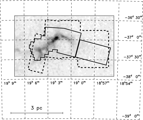
Figure 1. Coverage map for the Spitzer data taken in CrA. The thick black line shows the IRAC coverage in bands 1 and 3 (3.6/5.8 μm) and the thick black dotted line shows the MIPS 24 μm coverage. The underlying gray scale is a near-infrared extinction map created using 2MASS point sources.
Download figure:
Standard image High-resolution imageTable 1. Spitzer Observations of CrA
| Instrument | AOR ID | PID | Observation Date |
|---|---|---|---|
| IRAC | 0003650816 | 6 | 2004 Apr 20 |
| 0017672960 | 30784 | 2006 Sep 25 | |
| 0017673472 | 30784 | 2006 Sep 25 | |
| 0027041280 | 30574 | 2008 May 10 | |
| MIPS | 0003664640 | 6 | 2004 Apr 11 |
| 0017673216 | 30784 | 2007 May 30 | |
| 0017673728 | 30784 | 2007 May 29 | |
| 0027042816 | 30574 | 2008 Oct 23 |
Download table as: ASCIITypeset image
The basic calibrated data are downloaded from the Spitzer archive and processed by the team using the same, custom pipeline processing programs and techniques as used by c2d (see the c2d Final Delivery Document; Evans et al. 2007). Briefly, the data were inspected and custom masks were created to identify bad pixels and correct for instrumental effects. Mosaics were created from the improved data using the MOPEX package (Makovoz et al. 2006), and source extraction was performed using the c2dphot tool (Evans et al. 2007), which is a derivative of DoPHOT (Schechter et al. 1993). Source lists for detections at each wavelength were band-merged together with the Two Micron All Sky Survey (2MASS) catalog (Skrutskie et al. 2006) and cross identifications are accurate within 2'' (see Section 2.4 of the c2d Final Delivery Document; Evans et al. 2007). Also note that the final catalog is "band-filled" (see, e.g., the c2d Final Delivery Document) to produce flux estimates of objects that were not found in the original source extraction processing, but were detected in the other bands (see further discussion in Section 3). This procedure is described in detail in the delivery documentation for the c2d Final Delivery Document (Evans et al. 2007). Briefly, c2dphot fits the point-spread function (PSF) profile at the position of the known source. Note, however, that all these flux densities, flagged as band-filled in our tables, should be considered as "bad photometry," like the 5σ upper limits in this catalog.
Statistics for the sources detected in CrA with a signal-to-noise ratio (S/N) of at least 3 can be found in Table 2. This corresponds to selecting all sources with detection quality "A," "B," or "C" (S/N ⩾ 7, 5, and 3, respectively) in any of the IRAC bands from the final delivered catalogs (cf., the c2d Final Delivery Document).
Table 2. Detection Statistics (S/N ⩾ 3) in CrA
| Detected with/in... | Number of Detections |
|---|---|
| ...IRAC Band 1 | 73254 |
| ...IRAC Band 2 | 50096 |
| ...IRAC Band 3 | 11023 |
| ...IRAC Band 4 | 6381 |
| ...MIPS Band 1 | 1919 |
| ...MIPS Band 2 | 65 |
| ...MIPS Band 1 and Band 2 | 54 |
| ...2MASS (total) | 8974 |
| ...All four IRAC bands, but not 2MASS | 350 |
| ...2MASS alone | 4 |
| ...IRAC, but not 2MASS | 51745 |
| ...MIPS Band 1 and 2MASS KS | 557 |
Download table as: ASCIITypeset image
Figures 2 and 3 show color mosaics of the entire CrA region (mapped with IRAC and MIPS), using IRAC bands 2 (4.5 μm) and 4 (8.0 μm), and MIPS 24 μm (blue, green, and red, respectively). Figure 2 includes the Coronet region, the SE and SW filaments, and Figure 3 shows the less known region called the "streamer," positioned further to the southwest.
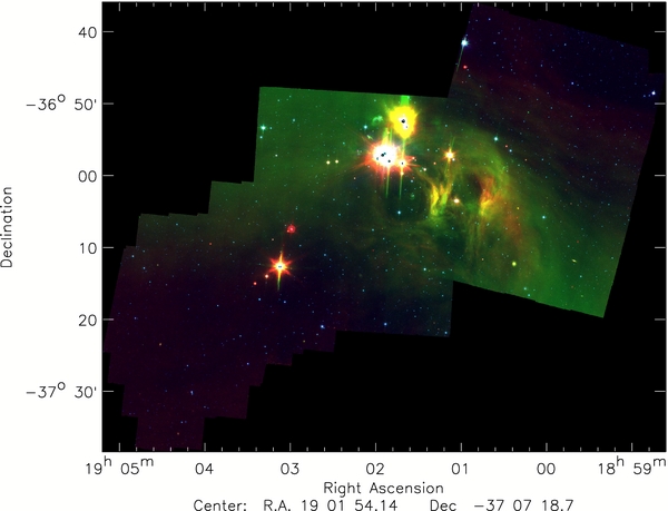
Figure 2. Three-color image of the main region in CrA, including the Coronet (bright white saturated region toward the center), made from the Spitzer IRAC 4.5 μm (blue), 8.0 μm (green), and MIPS 24 μm (red) bands.
Download figure:
Standard image High-resolution image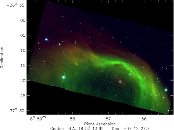
Figure 3. Three-color image of the streamer to the west of the main CrA region shown in Figure 2, made from the Spitzer IRAC 4.5 μm (blue), 8.0 μm (green), and MIPS 24 μm (red) bands.
Download figure:
Standard image High-resolution image2.2. Ancillary Submillimeter Array Observations
The regions around the previously identified YSOs IRS 5 (Wilking et al. 1997; Forbrich et al. 2006), IRS 7 (Wilking et al. 1997; Groppi et al. 2007), and IRAS 32 (IRAS 18595-3712; Wilking et al. 1992; Connelley et al. 2007; van Kempen et al. 2009) were observed with the SMA13 (Ho et al. 2004) in the dust continuum near 225 GHz (∼1.3 mm). Observations of the IRS 7 region were made on 2006 August 20 (program 2006-03-S046), while IRAS 32 and IRS 5 were observed on 2008 June 10 and 14 (program 2008A-S074). In this paper, we present only the continuum data for IRS 7, which were obtained as part of a line survey program; the results from that program will be reported elsewhere (J. E. Lindberg et al. 2011, in preparation). The data were edited and calibrated in the IDL-based software package MIR.14
For the observations of IRS 5 and IRAS 32, the SMA was in its compact-north configuration, with eight antennas, covering baselines of 16–139 m. The receiver's two sidebands were centered near 221 and 231 GHz. Chunks containing obvious spectral lines were removed before forming the continuum, resulting in a total continuum coverage of ∼3.6 GHz centered at 226 GHz. Observations of the quasar 3C 279 were used for bandpass calibration, and the quasars J1924-292 and J1937-399 were used for complex gain calibration. 3C 279 was used for absolute flux calibration, assuming a flux of 10.3 Jy based on observations at dates near in time to those that were flux calibrated using planets and moons.15
For the observations of the IRS 7 region, the SMA was in its compact configuration with six antennas, covering baselines of 16–69 m. A two-point mosaic pattern was used to cover the region. The receiver's two sidebands were centered near 219 and 229 GHz, with each sideband consisting of 24 overlapping chunks of 109 MHz each, or about 2 GHz for each sideband. Spectral lines were removed from the data, resulting in a total continuum coverage of ∼3.3 GHz centered at 224 GHz. Observations of the quasar 3C 454.3 were used for bandpass calibration, and the quasars J1924-292 and J1957-387 were used for complex gain calibration. Uranus was used for absolute flux calibration.
The MIRIAD software package was used for Fourier inversion of the visibilities, CLEAN deconvolution, and restoration with a synthesized beam. A Briggs robust weighting of 0 was used when mapping the continuum emission. The data were scaled by the inverse response of the primary beam ("primary-beam corrected"), to account for the loss of sensitivity away from the phase center. Synthesized beam sizes and 1 σ rms sensitivities are: 55 × 23 and 7.4 mJy for IRS 7, 46 × 26 and 3.7 mJy for IRS 5, and 37 × 22 and 4.4 mJy for IRAS 32, respectively.
2.3. Ancillary H2 Data
As a complement to the Spitzer and SMA data, we make use of multi-epoch H2 (2.12 μm) maps to detect jets and outflows in the CrA star-forming region to study their P.M.s and identify the exciting sources. Most of the data collected also have Ks or narrow-band filter images to remove the continuum from the H2 maps. The relevant information for these ancillary data is reported in Table 3.
Table 3. Journal of Observations—Ancillary Near-infrared Data
| Date of Obs. | Telescope/ | Filter | Resolution | Seeing | Exp. Time | FoV | Centered on/ |
|---|---|---|---|---|---|---|---|
| (yyyy mm dd) | Instrument | Band | ('' pixel−1) | ('') | (s) | (' × ') | Target |
| 2007 08 23 | ESO-NTT/SofI | H2, Ks | 0.29 | 1.3 | 1440, 290 | 10×10 | HH 734 |
| 2007 08 23 | ESO-NTT/SofI | H2, Ks | 0.29 | 1.3 | 1440, 290 | 10×10 | HH 730 |
| 2007 08 23 | ESO-NTT/SofI | H2, Ks | 0.29 | 1.3 | 1440, 290 | 10×10 | HH 101 |
| 2007 06 26 | ESO-NTT/SofI | H2, Ks | 0.29 | 1.1 | 1440, 290 | 10×10 | HH 99 |
| 2005 06 17 | ESO-VLT/ISAAC | H2, Ks | 0.15 | 0.8 | 500, 45 | 5×2.5 | IRAS 32 |
| 2005 06 16 | ESO-VLT/ISAAC | H2 | 0.15 | 0.8 | 4800 | 5×7 | R CrA |
| 2003 07 12 | ESO-VLT/ISAAC | H2, NB 2.09 | 0.15 | 0.9 | 1440, 290 | 6.3×6.3 | HH 101 |
| 2000 07 19 | ESO-VLT/ISAAC | H2 | 0.15 | 0.9 | 1200 | 6.8×6 | HH 99 |
| 1999 06 06 | ESO-NTT/SofI | H2, Ks | 0.29 | 0.8 | 600, 100 | 5.2×5.2 | R CrAa |
Note. aData already published in Caratti o Garatti et al. (2006).
Download table as: ASCIITypeset image
Our narrow-band H2 image archive is composed of data collected at ESO-NTT with SofI (Moorwood et al. 1998a) in 1999 (already published in Caratti o Garatti et al. 2006), and in 2007. Additional images were retrieved from the ESO science archive facility16 taken at the ESO-VLT with ISAAC (Moorwood et al. 1998b) in 2000, 2003, and 2005.
SofI 2007 images were observed in service mode between 2007 June and August, and cover four regions of CrA (∼10' × 10' each), mapping a total area of ∼20' × 17' (about one-tenth of the area mapped by Spitzer), for a total integration time of 5760 s. Figure 4 shows the area covered by the H2 mosaic.
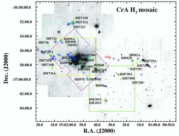
Figure 4. SofI (2007) H2 mosaic. Different polygons show regions mapped in different epochs (Yellow: 1999; Cyan: 2000; Green: 2003; Magenta: 2005). Known HH objects are indicated with green crosses. Newly detected H2 and Spitzer knots are also displayed as blue and red crosses, respectively.
Download figure:
Standard image High-resolution imageEarlier epoch maps enclose much smaller regions, centered on R CrA (ISAAC 2005 and SofI 1999, ∼5'×7' and 5 2×52 field of view (FoV), respectively), on HH 99 (ISAAC 2000, ∼68×6') or HH 101 (ISAAC 2003, 63×63), the details of which can be found in Table 3. These areas are indicated in Figure 4, where different polygons are superimposed on the SofI 2007 mosaic, showing regions mapped in different epochs (yellow: 1999; cyan: 2000; green: 2003; magenta: 2005). As a consequence, the P.M. analysis was mostly performed on knots inside and close to the Coronet region.
Finally, additional ISAAC images (H2 and Ks filters) around IRAS 18595-3712 (IRAS 32; located outside the SofI 2007 map), taken in 2005, were acquired to detect a possible H2 jet from that source.
All the raw data were reduced using IRAF packages applying standard procedures for sky subtraction, dome flat-fielding, bad pixel and cosmic ray removal, and making image mosaics. Continuum-subtracted images, H2–Ks and H2–NB(2.09 μm), were obtained by subtracting Ks and NB (2.09 μm) images, appropriately scaled and registered. Each pair of images was matched by means of tens to hundreds of field stars (depending on the mosaic size and crowding) selected excluding the YSO candidates. The scaling has been done by performing relative photometry on the selected stars. The images were not flux calibrated.
3. YSO SELECTION AND CLASSIFICATION
There are 45 sources in the observed Corona Australis region which were initially classified as YSO candidates from their Spitzer plus near-infrared colors using the technique outlined in Harvey et al. (2007, 2008, and references therein). This technique has been successfully adopted for the c2d and Gould Belt Spitzer surveys. Indeed, 33 out of the 45 sources in CrA (∼73%) have already been confirmed as YSOs in other studies (see Section 3.1 and Appendix A). Briefly, the selection method uses criteria based on a combination of infrared excess with a brightness limit in order to minimize extragalactic contamination. The selection method requires an S/N of 3 or higher detection in all four IRAC bands as well as in the MIPS 24 μm band. Figure 5 shows the color–magnitude space used to separate the YSO population in CrA from contaminants, which are mainly background giant stars and galaxies. To illustrate where the contaminating galaxy population is located in the same color–magnitude space, Figure 5 also shows color–magnitude diagrams for the full and re-sampled Spitzer Wide-area Infrared Extragalactic Survey (SWIRE) catalogs (Surace et al. 2004). The SWIRE observations were processed in exactly the same way as our data were processed in order to be used for a direct comparison (except that band-filling was not performed). Note that the SWIRE data are considerably deeper than ours, so the SWIRE catalog was trimmed down assuming the SWIRE observations had been obtained with sensitivities similar to those of our observations (this results in the "re-sampled SWIRE" catalog). A full discussion of the specifics of this process can be found in the c2d Final Delivery Document (Evans et al. 2007).
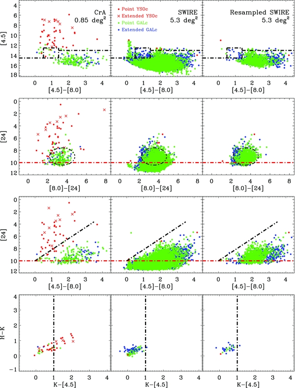
Figure 5. Color–magnitude diagrams showing the color space where YSOs are selected from Spitzer data along with the full SWIRE and re-sampled SWIRE catalogs. Based on the c2d YSO identification scheme by Harvey et al. (2007), where red and black dot-dashed lines are hard and fuzzy identification limits, respectively.
Download figure:
Standard image High-resolution imageTable 4 lists all YSO candidates selected through this method in CrA along with their Spitzer fluxes, known names, and classes (Lada 1987; Greene et al. 1994). Class is determined from the spectral slope, α, which is calculated over the widest range possible where data are available between 2.2 and 24 μm, and is defined as
The value of α is calculated from a linear fit to the logarithms, taking into account the uncertainties in the flux measurements. We classify sources with α ⩾ 0.3 as Class I, −0.3 ⩽ α < 0.3 as Flat spectrum, −1.6 ⩽ α < −0.3 as Class II, and α < −1.6 as Class III. Note that deeply embedded protostars, Class 0 sources, which require submillimeter data for identification, cannot be distinguished from Class I objects in this analysis.
Table 4. Sources Classified as YSO Candidates in CrA Based on Spitzer IRAC and MIPS
| ID | R.A. | Decl. | 3.6 μm | 4.5 μm | 5.8 μm | 8.0 μm | 24 μm | 70 μm | α | Other Namesa |
|---|---|---|---|---|---|---|---|---|---|---|
| (J2000) | (J2000) | (mJy) | (mJy) | (mJy) | (mJy) | (mJy) | (mJy) | (Class) | ||
| CrA-1 | 18 56 39.76 | −37 07 20.8 | 47.4 ± 2.4 | 38.8 ± 2.0 | 37.7 ± 1.8 | 42.6 ± 2.1 | 35.6 ± 3.3 | ... | −1.17 (II) | |
| CrA-2 | 18 57 52.63 | −37 14 40.1 | 2.04 ± 0.12 | 8.90 ± 0.44 | 35.8 ± 1.8 | 93.6 ± 4.6 | 171. ± 16. | 1690 ± 196 | 1.73 (G) | Leda Galaxy 90315 |
| CrA-3 | 18 59 43.92 | −37 04 0.11 | 1.69 ± 0.09 | 2.22 ± 0.11 | 2.93 ± 0.20 | 3.58 ± 0.19 | 6.97 ± 0.66 | ... | −0.18 (F) | ISO-CrA 551 |
| CrA-4 | 18 59 50.95 | −37 06 31.6 | 4.69 ± 0.25 | 3.93 ± 0.20 | 3.16 ± 0.17 | 2.79 ± 0.19 | 1.93 ± 0.22 | ... | −1.53 (II) | DENIS-J185950.9-370632 |
| CrA-5 | 19 00 15.55 | −36 57 57.7 | 1.07 ± 0.06 | 2.84 ± 0.15 | 5.79 ± 0.30 | 8.04 ± 0.40 | 13.3 ± 1.2 | ... | 0.51 (I) | ISO-CrA 761 |
| CrA-6 | 19 00 29.07 | −36 56 03.8 | 51.6 ± 2.7 | 36.0 ± 1.8 | 26.1 ± 1.3 | 18.5 ± 0.9 | 36.0 ± 3.3 | 52.0 ± 6.4 | −1.57 (II) | CrAPMS 82; GP g23 |
| CrA-7 | 19 00 38.94 | −36 58 14.7 | 40.8 ± 2.2 | 33.8 ± 1.7 | 25.8 ± 1.3 | 17.8 ± 0.9 | 4.49 ± 0.43 | ... | −2.08 (III) | ISO-CrA 931 |
| CrA-8 | 19 00 45.31 | −37 11 48.2 | 7.73 ± 0.40 | 6.66 ± 0.33 | 5.73 ± 0.29 | 6.85 ± 0.34 | 14.6 ± 1.4 | ... | −0.90 (II) | CrA-4444 |
| CrA-9 | 19 00 58.05 | −36 45 05.0 | 56.3 ± 3.3 | 43.8 ± 2.3 | 31.7 ± 1.5 | 25.1 ± 1.2 | 179. ± 17. | 154. ± 20.b | −1.04 (II) | |
| CrA-10 | 19 00 59.75 | −36 47 11.2 | 4.05 ± 0.22 | 3.95 ± 0.20 | 3.46 ± 0.18 | 3.87 ± 0.20 | 4.36 ± 0.41 | 35.3 ± 6.0 | −1.03 (II) | CrA-4324 |
| CrA-11 | 19 01 03.26 | −37 03 39.4 | 473. ± 29. | 335. ± 18. | 243. ± 12. | 174. ± 9. | 225. ± 21. | ... | −1.75 (III) | HD 176269; HR 71695 |
| CrA-12 | 19 01 16.29 | −36 56 28.3 | 8.69 ± 0.45 | 7.81 ± 0.38 | 6.77 ± 0.33 | 6.08 ± 0.29 | 7.46 ± 0.70 | ... | −1.23 (II) | V 667 CrA; CrA-41104 |
| CrA-13 | 19 01 18.95 | −36 58 28.4 | 36.5 ± 1.9 | 34.8 ± 1.8 | 36.2 ± 1.7 | 35.0 ± 1.7 | 52.8 ± 4.9 | 54.6 ± 7.2 | −0.92 (II) | CrA-4664; ISO-CrA 1271 |
| CrA-14 | 19 01 29.01 | −37 01 48.4 | 19.5 ± 1.0 | 13.8 ± 0.7 | 9.62 ± 0.48 | 6.61 ± 0.32 | 2.93 ± 0.29 | ... | −2.12 (III) | HH 101 IRS 16; G-947 |
| CrA-15 | 19 01 32.31 | −36 58 03.0 | 21.2 ± 1.1 | 18.9 ± 0.9 | 16.4 ± 0.8 | 13.8 ± 0.7 | 16.2 ± 1.5 | ... | −1.19 (II) | IRS 148; TS 2.98; G-877 |
| CrA-16 | 19 01 33.85 | −36 57 44.9 | 68.3 ± 5.1 | 70.9 ± 3.7 | 66.6 ± 3.2 | 71.9 ± 3.6 | 131. ± 12. | 173. ± 30. | −0.65 (II) | IRS 138; TS 2.88; G-857 |
| CrA-17 | 19 01 36.26 | −36 58 03.0 | 0.816 ± 0.047 | 0.678 ± 0.041 | 0.513 ± 0.128 | 0.340 ± 0.060 | 5.73 ± 0.92c | ... | ... | removed from list |
| CrA-18 | 19 01 40.41 | −36 51 42.3 | 49.0 ± 2.7 | 42.0 ± 2.1 | 41.3 ± 2.1 | 46.7 ± 2.8 | 118. ± 14. | ... | −0.70 (II) | G-657 |
| CrA-19 | 19 01 48.03 | −36 57 22.2 | 389. ± 24. | 798. ± 50. | 1270. ± 76. | 1810. ± 107. | 4500. ± 570.c | ... | 0.78 (I) | IRS 58; TS 2.48; MMS 129; SMM 410 |
| CrA-20 | 19 01 48.46 | −36 57 14.7 | 8.56 ± 0.51 | 26.2 ± 1.3 | 52.8 ± 3.5 | 80.9 ± 4.2 | 1110. ± 155.c | ... | 1.41 (I) | IRS 5N11 |
| CrA-21 | 19 01 51.12 | −36 54 12.4 | 30.3 ± 1.5 | 32.6 ± 1.7 | 37.2 ± 1.8 | 45.2 ± 2.2 | 39.9 ± 3.7 | ... | −0.68 (II) | IRS 88; TS 2.28 |
| CrA-22 | 19 01 51.86 | −37 10 44.7 | 3.75 ± 0.19 | 3.32 ± 0.17 | 2.79 ± 0.15 | 2.27 ± 0.13 | 1.79 ± 0.21 | ... | −1.47 (II) | |
| CrA-23 | 19 01 53.75 | −37 00 33.9 | 3.16 ± 0.17 | 2.96 ± 0.15 | 2.74 ± 0.17 | 3.01 ± 0.16 | 3.09 ± 0.34 | 113. ± 40.d | −1.09 (II) | Star A12 |
| CrA-24 | 19 01 55.60 | −36 56 51.1 | 11.0 ± 1.6 | 30.3 ± 3.2 | 54.0 ± 5.2 | 93.1 ± 13.5c | 297. ± 50.c | ... | 0.60 (I) | |
| CrA-25 | 19 01 57.27 | −36 52 05.0 | 0.588 ± 0.179c | 1.30 ± 0.38c | 1.43 ± 0.21 | 1.06 ± 0.32c | 3.22 ± 0.47c | ... | HH | removed from list |
| CrA-26 | 19 02 06.80 | −36 58 41.0 | 2.29 ± 0.12 | 2.22 ± 0.11 | 2.35 ± 0.14 | 2.48 ± 0.14 | 3.11 ± 0.64c | ... | −0.84 (II) | |
| CrA-27 | 19 02 10.44 | −36 53 44.5 | 6.94 ± 0.36 | 4.55 ± 0.23 | 3.55 ± 0.20 | 2.12 ± 0.11 | 0.962 ± 0.177 | ... | −2.24 (III) | |
| CrA-28 | 19 02 12.00 | −37 03 09.4 | 6.15 ± 0.31 | 5.04 ± 0.25 | 4.26 ± 0.22 | 4.62 ± 0.24 | 4.63 ± 0.45 | ... | −1.27 (II) | ISO-CrA 1431; G-147 |
| CrA-29 | 19 02 14.63 | −37 00 32.9 | 9.21 ± 0.49 | 11.4 ± 0.57 | 12.2 ± 0.59 | 11.8 ± 0.6 | 14.2 ± 1.3 | ... | −0.64 (II) | ISO-CrA 1451 |
| CrA-30 | 19 02 27.07 | −36 58 13.1 | 300. ± 17. | 242. ± 14. | 256. ± 13. | 248. ± 13. | 150. ± 14. | ... | −1.37 (II) | Hα 1413; HBC 68014 |
| CrA-31 | 19 02 33.07 | −36 58 21.2 | 356. ± 19. | 335. ± 20. | 347. ± 17. | 339. ± 17. | 238. ± 22. | 167. ± 18.d | −1.09 (II) | Hα 313; ISO-CrA 1591 |
| CrA-32 | 19 02 56.82 | −37 07 19.4 | 0.314 ± 0.018 | 0.374 ± 0.021 | 0.351 ± 0.039 | 0.234 ± 0.038 | 5.21 ± 0.92c | ... | ... | removed from list |
| CrA-33 | 19 03 01.03 | −37 07 53.4 | 7.04 ± 0.36 | 10.2 ± 0.5 | 15.3 ± 0.8 | 16.9 ± 0.8 | 32.9 ± 3.1 | ... | 0.06 (F) | IRAS 32d15 |
| CrA-34 | 19 03 09.16 | −36 57 22.0 | 149. ± 8. | 121. ± 6. | 92.2 ± 4.4 | 68.2 ± 3.4 | 20.4 ± 1.9 | ... | −2.02 (III) | ISO-CrA 1981 |
| CrA-35 | 19 03 11.84 | −37 09 02.1 | 19.6 ± 1.0 | 14.9 ± 0.7 | 11.7 ± 0.6 | 10.4 ± 0.5 | 11.7 ± 1.1 | ... | −1.46 (II) | ISO-CrA 2011 |
| CrA-36 | 19 03 24.29 | −37 15 07.7 | 44.9 ± 2.5 | 44.9 ± 2.3 | 52.1 ± 2.7 | 61.3 ± 3.0 | 132. ± 12. | 96.1 ± 9.7 | −0.39 (II) | |
| CrA-37 | 19 03 55.24 | −37 09 35.9 | 1.43 ± 0.07 | 1.95 ± 0.10 | 2.63 ± 0.14 | 3.84 ± 0.20 | 20.8 ± 1.9 | 78.1 ± 8.3d | 0.36 (I) | |
| CrA-38 | 18 58 56.40 | −37 07 37.9 | 519. ± 28. | 298. ± 17. | 264. ± 13. | 176. ± 9. | 51.3 ± 4.7 | ... | −2.21 (III) | ISO-CrA 131 |
| CrA-39 | 19 00 23.47 | −37 12 24.2 | 3.81 ± 0.33 | 2.21 ± 0.18 | 1.65 ± 0.15 | 1.96 ± 0.27 | 6.92 ± 0.72 | 943. ± 97.d | −0.95 (G) | 6dFGSgJ190023.5-37 |
| CrA-40 | 19 01 25.75 | −36 59 19.1 | 259. ± 18. | 223. ± 12. | 216. ± 11. | 170. ± 8. | 103. ± 10. | ... | −1.38 (II) | VSSt 1816 |
| CrA-41 | 19 01 41.62 | −36 59 52.7 | 298. ± 17. | 295. ± 16. | 293. ± 18. | 324. ± 16. | 293. ± 27. | ... | −1.04 (II) | Hα 213; HBC 67714 |
| CrA-42 | 19 01 50.48 | −36 56 38.4 | 106. ± 7. | 143. ± 9. | 179. ± 10. | 196. ± 12. | 348. ± 35. | ... | −0.39 (II) | IRS 68 |
| CrA-43 | 19 01 58.54 | −36 57 08.5 | 22.5 ± 1.3 | 72.1 ± 3.8 | 136. ± 8. | 195. ± 11. | 807. ± 78. | ... | 0.88 (I) | SMM210; CHLT 1517 |
| CrA-44 | 19 02 58.67 | −37 07 35.9 | 6.30 ± 0.71 | 17.2 ± 1.2 | 17.3 ± 1.1 | 12.9 ± 0.7 | 2040. ± 193. | 28500. ± 2870 | 1.66 (I) | IRAS 32c15 |
| CrA-45 | 19 03 16.09 | −37 14 08.2 | 223. ± 12. | 224. ± 12. | 256. ± 13. | 278. ± 14. | 676. ± 63. | 680. ± 69. | −0.42 (II) | VSSt 1016; IRAS 3415 |
Notes. aReferences are as follows: 1Olofsson et al. (1999); 2Walter et al. (1997); 3Glass & Penston (1975); 4López Martí et al. (2005); 5Knacke et al. (1973); 6Reipurth & Wamsteker (1983); 7Sicilia-Aguilar et al. (2008); 8Taylor & Storey (1984); 9Chini et al. (2003); 10Nutter et al. (2005); 11Forbrich & Preibisch (2007); 12Graham (1993); 13Marraco & Rydgren (1981); 14Herbig & Bell (1988); 15Wilking et al. (1992); 16Vrba et al. (1976a); 17Choi et al. (2008). bThe flux for CrA-9 was computed using aperture photometry from the 70 μm image; the catalog entry for this source shows it as a non-detection. See Appendix A.9. cThe flux for this source at this wavelength has been "band-filled" (described in Section 3). dThis 70 μm flux is listed in the catalog with a "P" flag, meaning that there were multiple catalog detections near this 70 μm source. The catalog source chosen to match the 70 μm detection gave the most "consistent" SED, and was also the one closest to the 70 μm detection (see the c2d Final Delivery Document; Evans et al. 2007).
It is important to note that the α quoted in the tables and in our catalogs is computed by selecting all valid wavelengths (having a quality of detection not "N" or "U," meaning a non-detection or an upper limit, respectively) in the combined epochs between Ks and 24 μm (up to six possible bands). Any fluxes or their uncertainties that are NaN, zero, or negative are excluded. In some cases, for the calculation of α, a band-filled flux has been used (in the c2d catalogs this is indicated as having an image type of "−2"). Band-filling typically happens for sources that have clear shorter wavelength IRAC fluxes, but are undetected at longer wavelengths (see the c2d Final Delivery Document; Evans et al. 2007). If a source in Table 4 has a band-filled flux, it will be indicated as such with a footnote.
The use of the terms "YSO" and "YSO candidate" will be somewhat interchanged throughout this paper. To be clear, not all the sources discussed as YSOs are spectroscopically identified YSOs or confirmed as members of the CrA cloud, although some of them have been through other studies. This is why the term "YSO candidate" is used most frequently when describing specific sources. Ample references to the literature are provided in the text, appendices, and the tables in order to facilitate further studies of these YSOs and YSO candidates.
3.1. Spitzer Classified YSO Candidates
There are 45 YSO candidates classified using the standard technique, as discussed above, and these are listed in Table 4. In two cases (CrA-2 and CrA-39), the candidates turned out to be known galaxies; they are discussed in Appendix A and appear in the table, although they are not counted in our final list of YSO candidates. There are also three YSO candidates which, upon visual inspection, were determined not to be YSOs: CrA-17, CrA-25 (which is likely a HH object), and CrA-32 (see descriptions for all in Appendix A). This gives a final total of 40 YSO candidates selected by our method with Spitzer. Many of the YSO candidates are known YSOs from the literature, but there are seven new YSO candidates (CrA-1, CrA-7, CrA-9, CrA-22, CrA-24, CrA-36, CrA-37) that have not been selected by any other survey, in most cases because the Spitzer observations extend beyond the region included in other surveys. CrA-24 is a new YSO candidate that is located within the Coronet, and further discussion of it can be found in A.24. For a more detailed description of each of the 45 sources selected using this method, see Appendix A.
The spectral energy distributions (SEDs) for the 45 sources are shown in Figure 6 (Class I and Flat spectrum candidates), Figure 7 (Class II candidates), and Figure 8 (Class III candidates). In these figures, the open circles represent the Spitzer and ancillary data, and the filled circles represent the dereddened fluxes (using the extinction law of Weingartner & Draine 2001, with RV = 5.5). In Figures 7 and 8, a gray line represents the photosphere of a K7 main-sequence star, and the dashed black line represents the average SED for T Tauri stars in Taurus (D'Alessio et al. 1999).

Figure 6. SEDs are shown for the Class I and Flat spectrum sources in CrA selected from the Spitzer data as discussed in Section 3.1. Open circles represent the Spitzer and ancillary data. The number that appears in each panel corresponds to the object number in Table 4. Note that sources CrA-2 (a known galaxy, see discussion in Appendix A.2) and CrA-32 (see discussion in Appendix A.32) have been removed from our sample of YSO candidates.
Download figure:
Standard image High-resolution image
Figure 7. SEDs are shown for the Class II sources in CrA selected from the Spitzer data as discussed in Section 3.1. Open circles represent the Spitzer and ancillary data, filled circles represent the dereddened fluxes, the gray line represents the stellar photospheric emission expected from the best-fit NextGen model, and the dashed black line represents the average SED for T Tauri stars in Taurus (D'Alessio et al. 1999). The number that appears in each panel corresponds to the object number in Table 4. Note that sources CrA-17 (see discussion in Appendix A.17), CrA-25 (see discussion in Appendix A.25), and CrA-39 (a known galaxy, see discussion in Appendix A.39) have all been removed from our sample of YSO candidates.
Download figure:
Standard image High-resolution image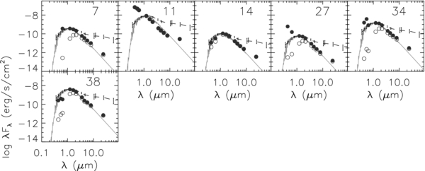
Figure 8. SEDs are shown for the Class III sources in CrA selected from the Spitzer data as discussed in Section 3.1. Open circles represent the Spitzer and ancillary data, filled circles represent the dereddened fluxes, the gray line represents the stellar photospheric emission expected from the best-fit NextGen model, and the dashed black line represents the average SED for T Tauri stars in Taurus (D'Alessio et al. 1999). The number that appears in each panel corresponds to the object number in Table 4. The fit to CrA-11 is not very good in the visible wavelength range because it has a known spectral type of B8V (see Appendix A.11), whereas the model assumes a spectral type of K7 (which is a reasonable approximation for most of the sources).
Download figure:
Standard image High-resolution image3.2. YSO Candidates Classified from 2MASS and MIPS
In some cases, there are regions covered by MIPS that are not covered in IRAC (or else are only covered in IRAC bands 1/3 and not in 2/4, and vice versa). To have as complete a sample as possible, we use 2MASS + the MIPS data in order to select additional YSO candidates. A Ks versus Ks − [24] color–magnitude diagram for CrA is shown in Figure 9. Following the analysis of Rebull et al. (2007) for Perseus and Padgett et al. (2008) for Ophiuchus, we find several new YSO candidates based on this diagram. The specific criteria used to select YSO candidates in this way are as follows: Ks < 14 mag, 24 μm < 9 mag, and Ks − [24] > 2. The region of the color–magnitude diagram that meets these criteria is outlined in Figure 9. There are 12 YSO candidates that meet these criteria, and they are listed in Table 5. However, as was the case for CrA-2, source CrA-50 is part of the extended galaxy Leda 90315, and so it has been rejected from the list of candidates (see also Appendix A.2 for a discussion of CrA-2). Thus we yield a total of 11 new YSO candidates from this technique, five of which have never been identified as candidate YSOs before.
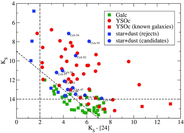
Figure 9. Ks vs. Ks − [24 μm] color–magnitude diagram for CrA. Symbols represent the following classifications: "Galc," or galaxies (green squares), YSO candidates that appear in Table 4 (filled red circles), and YSO candidates that turned out to be known galaxies (filled red squares). The phase space used to select star+dust sources as candidate YSOs, as discussed in Section 3.2, is shown by the dashed lines. Those star+dust sources that were rejected as candidate YSOs are represented by filled blue squares. The star+dust sources that met the criteria to be considered YSO candidates, and which appear in Table 5, are annotated and represented by filled blue circles.
Download figure:
Standard image High-resolution imageTable 5. Sources Classified as YSO Candidates in CrA Based on 2MASS and MIPS 24 μm
| ID | R.A.a | Decl.a | 3.6 μm | 4.5 μm | 5.8 μm | 8.0 μm | 24 μm | 70 μm | α | Other Namesb |
|---|---|---|---|---|---|---|---|---|---|---|
| (J2000) | (J2000) | (mJy) | (mJy) | (mJy) | (mJy) | (mJy) | (mJy) | (Class) | ||
| CrA-46 | 18 55 56.32 | −37 00 07.1 | ... | ... | ... | ... | 15.6 ± 1.5 | ... | −0.11 (F) | |
| CrA-47 | 18 56 40.28 | −36 55 20.8 | ... | ... | ... | ... | 4.46 ± 0.43 | ... | −1.04 (II) | |
| CrA-48 | 18 57 07.86 | −36 54 04.4 | ... | ... | ... | ... | 2.53 ± 0.26 | ... | −1.21 (II) | |
| CrA-49 | 18 57 22.48 | −37 34 42.5 | ... | ... | ... | ... | 3.00 ± 0.30 | ... | −0.96 (II) | |
| CrA-50 | 18 57 52.22 | −37 14 45.8 | 0.883 ± 0.053 | 0.567 ± 0.031 | 0.403 ± 0.060 | 0.286 ± 0.098c | 9.87 ± 1.87 | ... | −0.66 (G) | Leda Galaxy 90315 |
| CrA-51 | 18 59 34.26 | −37 21 41.5 | 1.26 ± 0.11 | ... | 0.848 ± 0.083 | ... | 5.69 ± 0.55 | ... | −0.49 (II) | |
| CrA-52 | 19 00 01.58 | −36 37 06.2 | ... | ... | ... | ... | 124.0 ± 11.5 | ... | −0.95 (II) | CrAPMS 71; HBC 6742; Hα 63 |
| CrA-53 | 19 01 11.49 | −36 45 33.8 | 5.99 ± 0.31 | ... | 3.49 ± 0.19 | ... | 4.35 ± 0.42 | ... | −1.31 (II) | LM10-14 |
| CrA-54 | 19 01 39.15 | −36 53 29.4 | 93.4 ± 4.9 | 59.4 ± 3.0 | 67.4 ± 23.9c | 131.0 ± 48.4c | 602. ± 101. | ... | −1.01 (II) | HD 176386B |
| CrA-55 | 19 01 55.23 | −37 23 41.0 | ... | ... | ... | ... | 1420. ± 134. | 1540. ± 161. | −0.51 (II) | DG CrA; HBC 2892; IRAS 245; |
| IRAS 18585-3728 | ||||||||||
| CrA-56 | 19 02 16.66 | −36 45 49.4 | 15.2 ± 0.8 | ... | 7.3 ± 0.4 | ... | 10.4 ± 1.0 | ... | −1.39 (II) | ISO-CrA 1466; CrA-41097; |
| DENIS-P J190216.6-364549 | ||||||||||
| CrA-57 | 19 03 25.48 | −36 55 05.3 | 12.4 ± 0.6 | ... | 5.74 ± 0.29 | ... | 5.43 ± 0.52 | ... | −1.60 (II) | ISO-CrA 2176 |
Notes. aCoordinates from our Spitzer catalog. bReferences are as follows: 1Walter et al. (1997); 2Herbig & Bell (1988); 3Marraco & Rydgren (1981); 4López Martí et al. (2010); 5Wilking et al. (1992); 6Olofsson et al. (1999); 7López Martí et al. (2005). cThis flux has a quality of detection of "D" meaning it has a 2 ⩽ S/N < 3. Fluxes that do not have this note all have a quality of detection of "A" (S/N ⩾7), "B" (S/N ⩾5), or "C" (S/N ⩾ 3).
Download table as: ASCIITypeset image
For the sources discussed in this section and in Section 3.1, the final list of Spitzer-selected sources includes 51 YSO candidates, 12 of which are new. Using the values of α defined at the beginning of Section 3, we find 10 Class I or Flat spectrum, 35 Class II, and 6 Class III candidate YSOs. This high fraction of Class II sources compared with other classes is consistent with that seen in the previously studied c2d star-forming regions (Evans et al. 2009).
3.3. Class III Population in CrA
While infrared surveys are excellent for identifying embedded YSOs still surrounded by circumstellar dust, they are less successful for classifying the Class III YSO population. Class III objects do not have the significant infrared excess associated with optically thick disks, and thus cannot be clearly distinguished from main-sequence stars. That is apparent from the analysis discussed in Section 3.1 (see Table 4), where only six Class III YSO candidates are identified. On the other hand, diskless Class III objects can be readily identified using X-ray observations in addition to the infrared (e.g., Grosso et al. 2000). Therefore, in order to obtain a census of the young population in CrA, we combine our Spitzer catalog with X-ray ROSAT data (B. M. Patten et al. 2011, in preparation) to select additional Class III YSO candidates. The completeness of our selected sample of Class III YSOs will be discussed in Section 3.5.
There are 34 ROSAT detections within our Spitzer CrA field. Of those, three do not have a Spitzer counterpart; two sources are off the main cloud and have Spitzer detections on the border of the positional uncertainty circle, so we do not make the association. The third (which is located within the high nebulosity region of TY CrA) is likely to be detected, but there are two Spitzer detections within the positional uncertainty, making the association ambiguous. Three ROSAT detections are the well known YSOs in CrA known as IRS 2, S CrA, and TY CrA. Six are YSO candidates that we classified as Class II or III using Spitzer and 2MASS: CrA-6, 11, 14, 16, 30, and 40 (see Table 4). Two Class II sources, CrA-52 and CrA-54 (listed in Table 5), were selected using Ks and 24 μm, as described in Section 3.2. The remaining 20 sources are listed in Table 6 as YSO candidates and are included in the clustering analysis later in this paper (see Section 4.2). All 20 of these sources are classified as "star" in our Spitzer catalogs (meaning they have SEDs that are well fitted by a reddened stellar photosphere) and have α values within the range of a Class III YSO, as calculated from their Spitzer + 2MASS SEDs.
Table 6. Class III YSO Candidates from Spitzer + ROSAT
| Spitzer ID | ROSAT IDa | Offsetb | R.A.c | Decl.c | 3.6 μm | 4.5 μm | 5.8 μm | 8.0 μm | 24 μm | α | Other Namesd |
|---|---|---|---|---|---|---|---|---|---|---|---|
| RX | ('') | (J2000) | (J2000) | (mJy) | (mJy) | (mJy) | (mJy) | (mJy) | |||
| CrA-58 | J1855.3-3730 | 6.26 | 18 55 18.91 | −37 29 56.7 | 1350. ± 77. | 804. ± 50. | 610. ± 34. | 338. ± 18. | 34.9 ± 3.2 | −2.86 | HD 175073; LTT 7499 |
| CrA-59e | J1857.5-3732 | 2.54 | 18 57 34.19 | −37 32 33.3 | ... | ... | ... | ... | 0.826 ± 0.144 | −2.76 | |
| CrA-60 | J1857.7-3719 | 13.1 | 18 57 45.15 | −37 19 37.9 | 32.0 ± 1.6 | 22.7 ± 1.1 | 15.7 ± 0.8 | 9.00 ± 0.43 | 0.882 ± 0.150 | −2.68 | [P98c] R01c1 |
| CrA-61 | J185802.3-365348 | 6.29 | 18 58 01.82 | −36 53 45.4 | ... | ... | ... | ... | 1.87 ± 0.21 | −2.82 | CrAPMS 52 |
| CrA-62f | J1858.7-3706 | 6.24 | 18 58 43.33 | −37 06 27.3 | 5980. ± 690.g | 2370. ± 286. | 3120. ± 158. | 1960. ± 111. | 228. ± 21. | −2.67 |  CrA; HR 7152; R041 CrA; HR 7152; R041 |
| CrA-63 | J185856.2-364032h | 4.35 | 18 58 56.51 | −36 40 29.7 | ... | ... | ... | ... | 0.976 ± 0.207 | −2.67 | [P98c] R17c1 |
| CrA-64 | J1859.2-3711 | 1.04 | 18 59 14.82 | −37 11 32.6 | 21.6 ± 1.3 | 14.6 ± 0.9 | 9.15 ± 0.52 | 5.90 ± 0.32 | 0.979 ± 0.138 | −2.74 | R021; CrAPMS 62; Hα 113 |
| CrA-65 | J190039.0-364805 | 8.17 | 19 00 39.30 | −36 48 12.3 | 27.2 ± 1.4 | 18.0 ± 0.9 | 12.4 ± 0.6 | 7.45 ± 0.37 | 0.898 ± 0.146 | −2.64 | R141; CrAPMS 92 |
| CrA-66 | J190109.4-364751 | 4.00 | 19 01 09.70 | −36 47 52.9 | 118. ± 7. | ... | 57.1 ± 2.8 | ... | 3.58 ± 0.34 | −2.79 | VSS VIII-274 |
| CrA-67 | J1901.4-3704 | 8.60 | 19 01 25.63 | −37 04 53.7 | 11.5 ± 0.6 | 8.56 ± 0.42 | 5.94 ± 0.29 | 3.70 ± 0.18 | 0.371 ± 0.163i,j | −2.40 | ISO-CrA 1335 |
| CrA-68 | J190126.8-365911 | 4.88 | 19 01 27.15 | −36 59 08.5 | 37.1 ± 2.0 | 26.2 ± 1.3 | 18.4 ± 0.9 | 11.0 ± 0.5 | 1.12 ± 0.18i | −2.62 | R07a1; ISO-CrA 1355 |
| CrA-69 | J190128.6-365933 | 1.82 | 19 01 28.71 | −36 59 31.8 | 95.1 ± 5.5 | 66.1 ± 3.4 | 47.7 ± 2.3 | 28.9 ± 1.4 | 2.86 ± 0.29 | −2.66 | ISO-CrA 1365; CXO 126 |
| CrA-70 | J190134.6-370058 | 3.27 | 19 01 34.84 | −37 00 56.5 | 258. ± 15. | 152. ± 8. | 111. ± 6. | 67.5 ± 3.4 | 7.87 ± 0.74 | −2.74 | CrAPMS 12; VSSt 137 |
| CrA-71 | J190139.0-370207 | 3.88 | 19 01 39.32 | −37 02 07.4 | 25.9 ± 1.4 | 16.8 ± 0.9 | 11.5 ± 0.6 | 6.65 ± 0.33 | 0.718 ± 0.193i | −2.64 | [GP75] R CrA o8 |
| CrA-72 | J190140.3-364429 | 4.20 | 19 01 40.55 | −36 44 32.0 | 91.9 ± 5.0 | ... | 40.9 ± 2.1 | ... | 2.92 ± 0.30 | −2.72 | VSS VIII-264 |
| CrA-73 | J190200.1-370227 | 4.93 | 19 02 00.11 | −37 02 22.1 | 13.7 ± 0.7 | 9.21 ± 0.46 | 6.38 ± 0.34 | 3.87 ± 0.22 | 0.491 ± 0.250i,k | −2.53 | Hα 133 |
| CrA-74 | J190201.7-370746 | 4.02 | 19 02 01.96 | −37 07 43.5 | 129. ± 7. | 76.6 ± 4.3 | 56.2 ± 2.7 | 31.6 ± 1.6 | 3.88 ± 0.38 | −2.79 | V702 CrA; CrAPMS 22 |
| CrA-75 | J190222.0-365541 | 1.41 | 19 02 22.12 | −36 55 40.9 | 65.4 ± 3.4 | 43.2 ± 2.2 | 30.5 ± 1.5 | 19.0 ± 0.9 | 2.22 ± 0.25 | −2.66 | VSSt 247; HBC 6799 |
| CrA-76 | J190249.7-364618 | 5.79 | 19 02 49.80 | −36 46 23.7 | 37.0 ± 2.0 | ... | 15.7 ± 0.8 | ... | 1.07 ± 0.17 | −2.69 | ISO-CrA 1745 |
| CrA-77 | J190408.2-370249 | 3.20 | 19 04 07.95 | −37 02 47.8 | 36.7 ± 2.0 | ... | 16.7 ± 0.8 | ... | 1.04 ± 0.15 | −2.76 | VSS VIII-214 |
Notes. aFrom B. Patten et al. (2010, private communication). The shorter coordinate names are sources from the PSPC (Position Sensitive Proportional Counter) catalog (they are less precise than the longer coordinate names). All the ROSAT IDs have a prefix of "RX." bOffset is calculated as the distance between our Spitzer position and the ROSAT position from Patten et al. (private communication). Note that the ROSAT positions are computed from centroiding using the PROS package in IRAF. cCoordinates from our Spitzer catalog. dReferences are as follows: 1Patten (1998); 2Walter et al. (1997); 3Marraco & Rydgren (1981); 4Vrba et al. (1976b); 5Olofsson et al. (1999); 6Forbrich & Preibisch (2007, CXO is the listing number from Table 2 of their paper); 7Vrba et al. (1976a); 8Glass & Penston (1975); 9Herbig & Bell (1988). eIn Table 13 of Fernández et al. (2008), CrA-59 (RX J1857.5-3732) is referred to as a binary, where the eastern component has a spectral type of M5 and the western component has a spectral type of M6. Only one source is detected in our Spitzer observations. Note that this source does not have any IRAC fluxes because it is off the field in the IRAC images (the MIPS field extends a little further). fPatten (1998) says this is not a member because it is an eclipsing binary and if you work out the numbers, it is likely foreground. This could be true because these are very bright fluxes. gThis flux is flagged "K" in the catalog meaning that it is complex, i.e., there are two or more detections within 2'' in the same band in the same epoch. The quality is likely still quite good, however. hThere is also a PSPC coordinate name for this source, RX J1858.9-3640, and although it is about 42'' away, it is the same source due to imprecise PSPC coordinates. iThe flux for this source at this wavelength has been "band-filled" (described in Section 3). jThis flux has a quality of detection of "D" meaning it has a 2 ⩽ S/N < 3. Fluxes that do not have this note all have a quality of detection of "A" (S/N ⩾ 7), "B" (S/N ⩾5), or "C" (S/N ⩾ 3). kThis flux is flagged "U" in the catalog indicating that it is an upper limit because it has been band-filled and has an S/N < 5.
Download table as: ASCIITypeset image
3.4. Known YSOs Not Classified with Spitzer
The Coronet is a well known young stellar cluster, with several YSOs previously studied by several authors at visible and near-infrared wavelengths. Unfortunately, this region is very bright in the longer wavelength Spitzer bands and many sources are saturated in our images, which may result in a band-filled flux. Therefore, we do not have enough SED coverage to classify them as YSO candidates (recall that we require an S/N of 3 or higher detection in all four IRAC bands as well as in the MIPS 24 μm band before even considering a source as a YSO candidate). Nevertheless, since we want to analyze the entire CrA population, these sources should be included in a comprehensive list of YSO candidates. We reviewed the literature to recover those YSOs (and YSO candidates) that are not already included in Tables 4, 5, and 6. Our findings are listed in Table 7.
Table 7. Spitzer Matches to Known YSOs and Candidate YSOs in CrA
| Namea | R.A.b | Decl.b | 3.6 μm | 4.5 μm | 5.8 μm | 8.0 μm | 24 μm | α | c2d Catalog | Other Namesc |
|---|---|---|---|---|---|---|---|---|---|---|
| (J2000) | (J2000) | (mJy) | (mJy) | (mJy) | (mJy) | (mJy) | (Class) | Designation | ||
| R CrA | 19 01 53.67 | −36 57 08.0 | ⋅⋅⋅d,e | ⋅⋅⋅d,e | 10500. ± 1980 | ⋅⋅⋅d,e | 76.1 ± 644.0d,e | −2.55 (III)f | star | TS 2.101; VSSt 12 |
| S CrA | 19 01 08.62 | −36 57 20.3 | 2580. ± 187. | 3040. ± 218. | 3510. ± 224. | 2640. ± 234. | <195d,e | −0.80 (II) | star+dust(IR1) | VSSt 32; SMM 73 |
| T CrA | 19 01 58.78 | −36 57 49.9 | 1930. ± 131. | 2110. ± 127. | 2360. ± 130. | 3520. ± 202. | ... | −0.35 (II) | rising | TS 4.31, VSSt 22 |
| VV CrA | 19 03 06.80 | −37 12 49.1 | 1570. ± 203. | 2900. ± 479. | 12200. ± 915. | 6770. ± 678. | <5800d,e | 0.36 (I) | rising | VSSt 42; SMM 93 |
| TY CrA | 19 01 40.81 | −36 52 33.8 | 844. ± 82. | 631. ± 59. | 1060. ± 114. | 2900. ± 372. | ... | −0.76 (II) | PAH-em | VSSt 52 |
| HD 176270 | 19 01 04.30 | −37 03 41.7 | 684. ± 42. | 468. ± 25. | 359. ± 18. | 190. ± 9. | 21.7 ± 2.1 | −2.81 (III) | star | HR 71704 |
| IRS 1g | 19 01 50.68 | −36 58 09.7 | 2960. ± 352. | 4520. ± 526. | 14000. ± 1150. | <150d,e | 22300. ± 4600.d | 0.92 (I) | rising | VSSt 152; TS 2.61 |
| IRS 2 | 19 01 41.56 | −36 58 31.2 | 1770. ± 235. | 2330. ± 239. | 6580. ± 375. | 7940. ± 506. | <1450d,e | 0.75 (I) | rising | TS 13.11; SMM 53 |
| IRS 7A (=7W) | 19 01 55.32 | −36 57 21.9 | 50.9 ± 4.5 | 239. ± 24. | 546. ± 43. | 1050. ± 78. | <2790d,e | 2.64 (I) | rising | |
| IRS 7B (=7E) | 19 01 56.40 | −36 57 28.1 | 36.7 ± 2.6 | 257. ± 18. | 697. ± 38. | 957. ± 51. | ... | 2.78 (I) | rising | |
| IRS 10 | 19 02 04.09 | −36 57 01.2 | 5.28 ± 0.31 | 4.49 ± 0.24 | 3.70 ± 0.37 | 2.66 ± 0.16 | 1.27 ± 0.83d,e | −1.48 (II) | star | TS 4.21; [HHD2008]A 5695 |
| IRS 11 | 19 01 41.89 | −36 56 58.4 | 3.77 ± 0.20 | 3.02 ± 0.15 | 2.32 ± 0.17 | 1.47 ± 0.13 | <1.9d,e | −1.77 (III) | star | TS 2.51; [HHD2008]A 3675 |
| IRS 15 | 19 01 47.89 | −36 59 30.1 | 7.76 ± 0.39 | 5.29 ± 0.27 | 4.66 ± 0.24 | 2.65 ± 0.14 | 0.0966 ± 0.5590d,e | −2.01 (III) | star | TS 13.41; GP n6 |
| VSSt 8 | 19 01 37.27 | −36 49 21.0 | 206. ± 11. | 131. ± 7. | 100. ± 5. | 62.3 ± 3.2 | 6.45 ± 0.61 | −2.67 (III) | star | TS 1.81; GP q6 |
| Hα 10 | 18 58 51.86 | −37 19 22.7 | 7.80 ± 0.39 | 4.70 ± 0.23 | 3.18 ± 0.17 | 2.04 ± 0.11 | 0.132 ± 0.136d,e | −2.68 (III) | star | HBC 6737 |
| Hα 15 | 19 04 17.25 | −36 59 03.2 | 20.5 ± 1.1 | ... | 13.4 ± 0.7 | ... | 17.3 ± 1.6 | −1.24 (II) | star+dust(IR3) | |
| ISO-CrA 46 | 18 59 31.79 | −36 50 26.3 | 39.1 ± 2.0 | 24.6 ± 1.2 | 17.7 ± 0.9 | 10.5 ± 0.5 | 1.11 ± 0.17 | −2.70 (III) | star | |
| ISO-CrA 53 | 18 59 40.99 | −36 56 01.4 | 18.9 ± 0.9 | 11.5 ± 0.6 | 7.85 ± 0.39 | 4.79 ± 0.24 | 0.399 ± 0.154d,h | −2.73 (III) | star | [P98c] R13a8 |
| ISO-CrA 140 | 19 02 10.03 | −36 56 49.0 | 1.32 ± 0.08 | 1.40 ± 0.09 | 1.35 ± 0.31 | 0.662 ± 0.097d | 0.375 ± 0.290d,e | −1.66 (III) | star | 185847.7-3701119 |
| ISO-CrA 177 | 19 02 54.64 | −36 46 19.2 | 14.5 ± 0.7 | ... | 11.9 ± 0.6 | ... | 11.2 ± 1.0 | −1.19 (II) | star+dust(IR3) | CrA-410710 |
| CXO 23 | 19 01 43.07 | −36 50 18.9 | 0.549 ± 0.032 | 0.370 ± 0.023 | 0.279 ± 0.054 | 0.121 ± 0.104d,e | 0.178 ± 0.230d,e | −2.18 (III) | star | |
| CXO 34 | 19 01 55.77 | −36 57 27.5 | 11.1 ± 1.1 | 41.3 ± 2.7 | 71.5 ± 4.0 | 66.5 ± 5.0 | ... | 0.87 (I) | cup-down | |
| CXO 37 | 19 01 57.40 | −37 03 11.8 | 3.00 ± 0.16 | 2.31 ± 0.12 | 1.67 ± 0.10 | 1.03 ± 0.07 | 0.150 ± 0.206d,e | −2.10 (III) | star | 185834.7-3707359 |
| CXO 38 | 19 01 58.32 | −37 00 26.7 | 3.25 ± 0.16 | 2.68 ± 0.15 | 2.19 ± 0.14 | 1.30 ± 0.09 | 0.045 ± 0.258d,e | −1.71 (III) | star | G-3211; 185835.7-3704509 |
| CXO 42 | 19 02 01.96 | −36 54 00.0 | 0.292 ± 0.026 | 0.258 ± 0.024 | 0.217 ± 0.140d,e | 1.04 ± 0.10 | 3.31 ± 0.35 | 0.38 (I) | red | 185839.6-3658239 |
| CrA-205 | 19 01 11.72 | −37 22 21.5 | ... | 2.89 ± 0.16 | ... | 1.06 ± 0.09 | 0.163 ± 0.153d,e | −2.49 (III) | star | |
| CrA-452 | 19 00 44.55 | −37 02 11.0 | 24.4 ± 1.2 | 16.5 ± 0.8 | 11.7 ± 0.6 | 7.01 ± 0.35 | 0.951 ± 0.236d | −2.52 (III) | star | ISO-CrA 9812 |
| CrA-453 | 19 01 04.62 | −37 01 29.4 | 5.74 ± 0.29 | 4.31 ± 0.22 | 3.03 ± 0.15 | 1.82 ± 0.10 | 0.00174 ± 0.13000d,e | −2.36 (III) | star | CXO 113 |
| CrA-468 | 19 01 49.35 | −37 00 28.6 | 8.30 ± 0.42 | 5.94 ± 0.29 | 3.91 ± 0.20 | 2.32 ± 0.12 | 0.453 ± 0.256d,e | −2.52 (III) | star | CXO 2613; LS-RCrA 214 |
| CrA-4108 | 19 02 09.67 | −36 46 34.5 | 7.85 ± 0.42 | ... | 3.88 ± 0.20 | ... | 0.351 ± 0.173d,e | −2.40 (III) | star | ISO-CrA 14112 |
| CrA-4111 | 19 01 20.85 | −37 03 02.9 | 4.16 ± 0.22 | 3.08 ± 0.15 | 2.16 ± 0.12 | 1.35 ± 0.09 | 0.568 ± 0.186 | −2.29 (III) | star_no_MP1 | CXO 713 |
| Haas 4 | 19 01 40.67 | −36 56 04.9 | 0.978 ± 0.068 | 1.41 ± 0.09 | 1.38 ± 0.12 | 1.77 ± 0.29 | 0.458 ± 0.338d,e | −0.28 (F) | cup-down | |
| Haas 7 | 19 01 43.67 | −36 57 17.2 | 0.477 ± 0.032 | 0.426 ± 0.030 | 0.284 ± 0.071 | 0.127 ± 0.095d,e | <35d,e | −1.70 (III) | star | |
| Haas 17 | 19 01 51.74 | −36 55 14.2 | 0.724 ± 0.066 | 0.579 ± 0.038 | 0.484 ± 0.081 | 0.236 ± 0.125d,e | <8.3d,e | −1.48 (II) | star | |
| Haas 33 | 19 02 00.85 | −36 58 50.6 | 2.02 ± 0.11 | 1.36 ± 0.07 | 1.11 ± 0.09 | 0.619 ± 0.069 | <5d,e | −2.17 (III) | star | 185838.4-3703129 |
| Haas 34 | 19 02 01.41 | −36 58 51.7 | 0.685 ± 0.042 | 0.445 ± 0.031 | 0.407 ± 0.065 | 0.220 ± 0.059 | <4d,e | −2.02 (III) | star | 185838.9-3703149 |
| LS-RCrA 1i | 19 01 33.56 | −37 00 30.3 | 1.25 ± 0.07 | 1.20 ± 0.06 | 1.33 ± 0.09 | 2.01 ± 0.12 | 12.2 ± 1.2 | −0.08 (F) | Galc_star+dust(IR2) | G09 CrA-1815 |
| G09 CrA-9 | 19 01 58.32 | −37 01 06.0 | 0.302 ± 0.019 | 0.453 ± 0.028 | 0.469 ± 0.055 | 0.336 ± 0.051 | 0.0422 ± 0.2480d,e | −0.55 (II) | cup-down | |
| G09 CrA-11 | 19 01 01.11 | −36 58 34.5 | 1.08 ± 0.06 | 0.777 ± 0.042 | 0.544 ± 0.044 | 0.162 ± 0.061h | 0.0151 ± 0.1610d,e | −2.38 (III) | star | |
| GP pj | 19 01 38.91 | −36 53 26.4 | 583. ± 33. | 366. ± 23. | 272. ± 50.d | 296. ± 74.d | ... | −2.63 (III) | star | HD 176386 |
| GP wak | 19 02 22.43 | −36 55 38.6 | 14.2 ± 1.1l | 10.3 ± 0.5 | 6.78 ± 0.35 | 4.14 ± 0.23 | 0.316 ± 0.208d,e | −2.44 (III) | star | CrAPMS 3B16 |
| LM10-2 | 19 01 39.11 | −37 00 17.3 | 6.24 ± 0.32 | 4.70 ± 0.24 | 3.33 ± 0.19 | 2.07 ± 0.12 | 0.317 ± 0.224d,e | −2.19 (III) | star | 185816.6-3704399 |
| LM10-3 | 19 01 51.80 | −37 10 47.9 | 14.8 ± 1.0 | 10.1 ± 0.5 | 6.77 ± 0.34 | 3.99 ± 0.21 | 0.088 ± 0.208d,e | −2.52 (III) | star | |
| LM10-4 | 19 02 07.68 | −37 11 55.9 | 4.35 ± 0.23 | 3.14 ± 0.16 | 2.40 ± 0.13 | 1.33 ± 0.08 | 0.302 ± 0.169d,e | −2.30 (III) | star | |
| LM10-5 | 19 02 39.40 | −36 53 11.2 | 6.11 ± 0.31 | 4.23 ± 0.21 | 3.02 ± 0.19 | 1.74 ± 0.10 | 0.229 ± 0.153d,e | −2.44 (III) | star | ISO-CrA 16312 |
Notes. aThe name listed in this column can be used to search for the source in SIMBAD, except in the following cases: IRS (Taylor & Storey 1984), Hα (Marraco & Rydgren 1981), CXO (Forbrich & Preibisch 2007, listing number from their Table 2), CrA- (López Martí et al. 2005); Haas (Haas et al. 2008, listing number from their Table 3); G09 CrA- (Gutermuth et al. 2009, listing number from their Table 4); GP (Glass & Penston 1975); LM10- (López Martí et al. 2010). There are three known YSOs that do not appear in this list because they do not have Spitzer counterparts. These sources are (SIMBAD coordinates in J2000): IRS 9 (R.A.: 19 01 52.63, decl.: −36 57 00.2; Taylor & Storey 1984), SMA 2 (RS 9) (R.A.: 19 01 55.28, decl.: −36 57 16.6; Brown 1987), and Anon 2 (R.A.: 19 01 06.92, decl.: −36 58 07.3; Knacke et al. 1973). bCoordinates from our Spitzer catalog. cReferences are as follows: 1Taylor & Storey (1984); 2Vrba et al. (1976a); 3Nutter et al. (2005); 4Knacke et al. (1973); 5Haas et al. (2008); 6Glass & Penston (1975); 7Herbig & Bell (1988); 8Patten (1998); 9Wilking et al. (1997); 10López Martí et al. (2005); 11Sicilia-Aguilar et al. (2008); 12Olofsson et al. (1999); 13Forbrich & Preibisch (2007); 14Fernández & Comerón (2001); 15Gutermuth et al. (2009); 16Walter et al. (1997). dThe flux for this source at this wavelength has been "band-filled" (described in Section 3). eThis flux is flagged "U" in the catalog indicating that it is an upper limit because it has been band-filled and has an S/N < 5. fDue to band-filling and saturation, the spectral index for R CrA has been derived from the Ks and 5.8 μm bands alone. Its value and resulting classification are likely incorrect. It should be noted that R CrA has long been known to be a PMS star with an accretion disk (e.g., Knacke et al. 1973), and an SED slope of a Class II (Hillenbrand et al. 1992). gIRS 1 is the only source in this table that has a 70 μm flux in the catalog; it is an excellent "A" quality flux with a value of: 33700.±4700. hThis flux has a quality of detection of "D" meaning it has a 2 ⩽ S/N < 3. Fluxes that do not have this note all have a quality of detection of "A" (S/N ⩾7), "B" (S/N ⩾5), or "C" (S/N ⩾ 3). iDiscussed in Fernández & Comerón (2001). jThis source is a double with CrA-54 (HD 176386B). kThis source name comes from Wilking et al. (1997); it is located to the northeast of source GP w (called GP wb in the same paper, where GP is from Glass & Penston (1975)) and was also seen by Walter et al. (1997) who call the two sources CrAPMS 3 and 3B. CrAPMS 3 is also a YSO candidate, and can be found in Table 6 as CrA-75. It seems that in Meyer & Wilking (2009) there was some confusion when referring to GP wa - in that paper, it actually corresponds to our CrA-75. lThis flux is flagged "K" in the catalog meaning that it is complex, i.e., there are two or more detections within 2'' in the same band in the same epoch. The quality is likely still quite good, however.
In Table 7, we summarize the known YSOs along with the coordinates and fluxes of their Spitzer counterparts as well as information on how they are classified in the delivered catalog. Many of the most massive stars in CrA were added in this way, including R CrA. In the case of R CrA, because many of the Spitzer bands are saturated, α is computed from the K and 5.8 μm bands alone, resulting in a classification of Class III. However, it should be noted that R CrA has long been known to be a pre-main-sequence (PMS) star with an accretion disk (e.g., Knacke et al. 1973) and an SED slope of a Class II (Hillenbrand et al. 1992). In addition, there are three known YSOs in CrA that do not have a counterpart in our Spitzer catalog: IRS 9, SMA 2, and Anon 2 (also known as VSSt 14 and HBC 675). In the case of IRS 9 and SMA 2, the nebulosity from R CrA is too bright to distinguish the sources, and in the case of Anon 2, it is a diffraction spike from S CrA that causes a problem. IRS 9 is classified as a Class I (and detected with Chandra; Forbrich & Preibisch 2007), and SMA 2 is classified as a Class 0 (Groppi et al. 2007). Whether or not Anon 2 is a YSO is debated: both Patten (1998) and Neuhäuser et al. (2000) claim it is not a young member (lithium is not detected in its spectrum; Neuhäuser et al. 2000). Unfortunately, without the Spitzer fluxes available, we cannot determine a classification for Anon 2.
Not all sources that have ever been identified as a candidate YSO are included in Table 7. For example, IRS 3 and IRS 4 are not included because they are spectroscopically recognized as background giants (Meyer & Wilking 2009). Additionally, any candidate YSOs in the literature that our Spitzer observations classify as a galaxy (noted as "Galc" in the catalog) are not included. There is an exception to this, and that is when additional observations show that a source classified as "Galc" in our catalog should be a member, as in the case of LS-RCrA 1 (discussed at the end of this section).
Moreover, we compare our candidates to the Haas et al. (2008) list (their Table 3), which was selected using a millimeter excess technique. Of those 38 candidates, 8 are already included in our tables. There are five sources in their list which are classified in our Spitzer GB catalogs with SED slopes described as "star" or "cup-down," and their fluxes are reasonable enough (i.e., are not band-filled and have good quality detections) to include them as candidate YSOs in Table 7. Note that a "cup-down" classification means that the SED has a shape that is convex and cannot be classified by any other category (see the c2d Final Delivery Document; Evans et al. 2007). However, many of the remaining sources are listed in our catalog as "one" or "two," meaning they are only detected in one or two of the IRAC bands (generally in the 3.6 μm and/or 4.5 μm bands). Because there is such little information in the Spitzer bands for a proper classification, none of these sources has been included in our Table 7.
Finally, Table 7 also reports 2 out of 35 sources (namely G09 CrA-9, 11; from their Table 4) classified as candidate YSOs in Gutermuth et al. (2009) that are not included in our previous tables. Gutermuth et al. (2009) used Spitzer data of CrA available from the GTO PID 6 program (see Table 1), which is included in the area studied in this paper, but covers a much smaller field, and adopted a slightly different selection technique. They found 35 YSO candidates in the region covered by PID 6, and of those, 25 are also selected by our method to be YSO candidates. Two of their sources have been added to our Table 7: G09 CrA-11, which we classify as "star", and G09 CrA-9, which we classify as "cup-down." Of the remaining eight candidates, four are known YSOs that already appear in Table 7 (IRS 7A, IRS 7B, S CrA, and T CrA) and four are classified as "Galc" in our catalog. However, one of the "Galc" sources is a star of late spectral type, LS-RCrA 1 (Fernández & Comerón 2001), and thus has also been included in Table 7.
Table 7, along with Tables 4, 5, and 6, are intended to make up the most comprehensive list of YSOs and YSO candidates in CrA to date. The sources included in these tables (minus those sources identified as likely galaxies) will be used to analyze clustering in CrA (Section 4.2) and to determine the driving sources for the outflows/jets (Section 6.3).
The total number of candidate YSOs in CrA is 116, where 14 are classified as Class I, 5 are Flat spectrum, 43 are Class II, and 54 are Class III. All 116 sources are shown overlaid on a 24 μm image in Figure 10.

Figure 10. All 116 YSO candidates are overlaid on a 24 μm image; the image inset is the Chandra X-ray image of the Coronet (the blue square near the center is R CrA). The Class I (+) and Flat spectrum (×) sources are shown in red, Class II (diamond) sources are shown in green, and Class III (square) sources are shown in blue. The contour shown is the extinction map made from 2MASS + Spitzer data with levels AV = [5, 10, 15, 20]. This extinction map has a resolution of 180''. Most Class I/Flat sources are located in the high-density cluster, while Class II and III sources are found spread further out.
Download figure:
Standard image High-resolution image3.5. Completeness
Evans et al. (2007, 2009) estimated that the c2d (and similarly, GB) selected sample of YSO candidates is 90% complete down to a luminosity of 0.05 L☉, integrated from 1 to 30 μm at a distance of the Serpens star-forming region (260 pc). However, the observing strategy for CrA is slightly different from the rest of the GB regions because it was originally observed as part of a GTO program. There is only one epoch, as opposed to the usual two, and therefore the photometric depth is ∼30% less. Accounting for the difference in photometric depth and scaling for the distance of CrA (130 pc), we estimate that our 2MASS/Spitzer sample, selected using the c2d/GB method (discussed in Section 3.1 and reported in Table 4), is ∼90% complete down to ∼0.015 L☉.
To illustrate the completeness of the CrA sample, we constructed bolometric luminosity functions for the Class II and III candidates (Figure 11; see also Merín et al. 2008; Spezzi et al. 2011). First, we estimate the bolometric luminosity of the YSO candidates by integrating over all the observed SED data points, assuming a distance of 130 pc to CrA. The solid line in Figure 11 indicates the bolometric luminosity distribution of Class II and III YSO candidates discussed in Section 3.1 (and reported in Table 4) rebinned to a 0.03 size bin. Then, following the Harvey et al. (2007) method, we apply the c2d completeness correction to the sample of sources selected using the c2d/GB method discussed in Section 3.1. The Harvey et al. (2007) completeness correction compares, for each luminosity bin, the number of counts from a trimmed version of the deep SWIRE catalog of extragalactic sources with the number of counts for the c2d catalogs in Serpens. The completeness correction estimate is then applied to the five molecular clouds observed by c2d.

Figure 11. Bolometric luminosity function for the YSO candidates in CrA selected using the c2d/GB method (discussed in Section 3.1, solid line), with the completeness correction included for comparison (dashed line), as discussed in Section 3.5. In addition, the bolometric luminosity function for all YSO candidates is shown (dotted line).
Download figure:
Standard image High-resolution imageFor all the regions in the GB survey, this completeness correction translates since they are homogeneous in terms of photometric depth. However, as stated previously, this is not precisely the case for CrA. If we assume that the c2d/GB survey samples are homogeneous with CrA down to ∼0.015 L☉, the completeness correction, indicated by dashed lines in Figure 11, provides a completeness estimate of ∼90%. We would like to emphasize here that CrA is peculiar when compared with the c2d and GB star-forming regions previously studied in terms of the initial observing strategy and mostly because of various observational limitations (discussed in detail in the following paragraphs), which led to the inclusion of many additional YSO candidates selected using different techniques (see Sections 3.2, 3.3, and 3.4). To address the inclusion of these sources quantitatively, the bolometric luminosity function for all sources is overplotted in Figure 11 (dotted lines). However, because of the addition of these sources, the final sample of YSO candidates was not uniformly selected, and therefore we cannot speak to the completeness of the sample as a whole. It is clear from Figure 11 that many YSO candidates in CrA are not selected using solely the c2d/GB method, and we enumerate the reasons why in the following paragraphs.
The greatest sources of incompleteness in the standard c2d/GB method (Section 3.1) manifest in four ways. First, very low luminosity objects may be lost in the group of extragalactic sources. An additional bias originates from the Coronet region, with its bright, diffuse nebula. Second, in Section 3.2 we discussed the addition of YSO candidates based on their 2MASS + MIPS 24 μm photometry because they were not covered in IRAC (or else are only covered in IRAC bands 1/3 and not in 2/4, and vice versa). These sources (see Table 5) were not selected by the standard technique because the method requires detections in all four IRAC bands. Third, as discussed briefly in Section 3.4, the brightest sources (e.g., R CrA), which saturate the camera arrays, were not selected as YSO candidates by the c2d/GB method due to poor photometry and subsequent flux measurements. To remedy such incompleteness, we added known YSOs and YSO candidates from the literature (see Section 3.4 and Table 7). Finally, in order to select a sample of YSO candidates with a minimum of contamination from extragalactic sources and background stars, the c2d/GB method required at least a small infrared excess component. Therefore, as mentioned in Section 3.3, our method fails to detect PMS objects that do not have infrared excess, but still have some accretion activity, indicated by X-ray emission, Hα emission, etc. Consequently, the sample of Class III candidates in Table 4 is heavily biased, missing many Class III candidates. To correct this bias, we used the ROSAT data to include additional Class III candidates (see Table 6).
As discussed in Section 3.3, there are 34 ROSAT detections within our Spitzer field for CrA, of which 31 have Spitzer counterparts. To assess the completeness of the ROSAT All-Sky Survey at the distance of CrA, we determine the limiting unabsorbed X-ray luminosities for different levels of foreground extinction. Sources listed in the Faint Source Catalog have a minimum of six counts, corresponding to a limiting count rate of about 0.03 s−1 for a typical exposure time of 218 s. The typical exposure time is the median exposure time of Faint Source Catalog sources within 3° of R CrA. To find the limiting unabsorbed X-ray fluxes and luminosities, we simulate X-ray sources with assumed spectra using PIMMS (Mukai 1993). The spectra are assumed to be absorbed APEC thermal plasma spectra. The visual extinction of newly identified T Tauri stars in Neuhäuser et al. (2000) is AV < 1 mag, which is the value that we are assuming for this estimate, after conversion into absorbing hydrogen column densities using the empirical relation NH(cm−2) ≈ 2 × 10²¹ × AV (mag) (e.g., Ryter 1996; Vuong et al. 2003). Conservatively assuming a plasma temperature of 1 keV (∼10 MK; e.g., Feigelson et al. 2005), the limiting luminosity is log (LX) = 30.2 erg s−1 for AV = 1 mag, assuming a distance of 130 pc.
Subsequently, we use the cumulative X-ray luminosity distribution functions derived for subsets of the PMS population of the Orion Nebula Cluster (Preibisch & Feigelson 2005) to estimate the completeness of the ROSAT data for G, K, and M PMS stars. The limiting unabsorbed X-ray luminosity determined above corresponds to a completeness of 60%–70% for G and K stars and 20% for M stars. For the deep Chandra data, Forbrich & Preibisch (2007) quote a considerably better limiting luminosity of 4.3×1026 erg s−1 for no intervening extinction which would be complete for all G, K, and M PMS stars. Assuming a foreground extinction of AV = 10 mag yields a limiting luminosity of 6.1×1027 erg s−1 for five-count detections, still complete for all G, K, and M PMS stars. For our purposes, the Chandra data are complete for the PMS population of the inner Coronet, while the much less sensitive ROSAT data still yield a good estimate of the outlying YSO population.
4. DISTRIBUTION OF YSOs
4.1. Extinction Map and YSO Distribution
With a census of the YSOs in CrA, we can examine the spatial distribution of the sources with respect to each other and the dense gas. Usually such a distribution reflects the underlying structure of the cloud, providing us with clues about the physical processes responsible for its creation. In particular, it can be of help in discriminating between two well known basic structures: hierarchical-type clusters and centrally condensed embedded clusters (see, e.g., Lada & Lada 2003, and references therein). In the first case, clouds exhibit surface density distributions with multiple peaks and more complex shapes, whereas the centrally condensed clusters have a highly concentrated surface density distribution with a relatively smooth radial profile (ρ* ∼ r−a). Moreover, the latter usually correlates with mass segregation, with massive stars found near the cluster center (see, e.g., Lada & Lada 2003, and references therein).
In Figure 10, all 116 YSO candidates are overlaid on the 24 μm mosaic, along with contours showing the extinction map we have created as part of the data pipeline using 2MASS and Spitzer data. To make this map, the line-of-sight visual extinction (AV) is estimated for each source classified in the catalog as a "star" (e.g., sources classified as YSO candidates are excluded) based on its SED from 1.25 to 24 μm, adopting the Weingartner & Draine (2001) RV = 5.5 extinction law, which has been shown to be consistent with data from the c2d/GB studies (Chapman et al. 2009; Chapman & Mundy 2009). These line-of-sight extinctions are then convolved with uniformly spaced Gaussian beams (with FWHM = 180'') to construct the extinction map (refer to Evans et al. 2007, for details). The mean AV in our CrA map is ∼5 mag, and the maximum AV is ∼30 mag, which is found in the Coronet region. The AV values in our map have not been corrected for any extinction offsets because a nearby off-cloud field was not imaged for comparison, and may be systematically high by as much as 1–2 mag (see Table 27 in Evans et al. 2007). For comparison, the extinction map presented by Gutermuth et al. (2009, and shown in our Figure 1), which is based only on 2MASS observations, exhibits a mean AV of ∼0.3 mag and maximum AV of ∼20 mag over the same region covered by our Spitzer observations. The lower values can perhaps be explained by the use of a different extinction law, RV = 3.1 (Rieke & Lebofsky 1985), for the near-infrared observations. Correcting for the different extinction laws, the near-infrared extinction map would have AV values that are ∼25% higher.
As can be seen in Figure 10, the morphology of the entire region is mainly a clustered one, extending toward the southeast, although the stars are mainly clustered near the Coronet, which indeed harbors a Herbig Ae star (R CrA) in its very center. It is striking how the Class I sources (red +) are found in the highest extinction regions, highly clustered in the Coronet, the Class II sources (green diamonds) are spread a little further out, and the Class III sources (blue squares), spread even further out into the molecular cloud, forming a sort of halo around the Class I and Class II sources. A distribution where the Class I sources are more densely clustered than the Class II sources is consistent with observations of other nearby star-forming regions such as Lupus, Serpens, and NGC 1333 (e.g., Merín et al. 2008; Gutermuth et al. 2008, 2009; Winston et al. 2009; Bressert et al. 2010). A quantitative analysis of the clustering in CrA will be discussed in Section 4.2.
4.2. Clustering Analysis
Using all 116 YSO candidates selected and/or compiled in this paper (see Figure 10) and listed in Tables 4, 5, 6, and 7, we perform the clustering analysis identical in method to that presented in Gutermuth et al. (2009) for comparison. The sample sizes are different because Gutermuth et al. (2009) used only the Spitzer data of CrA available from the GTO PID 6 program (see Table 1), which covers a much smaller FoV than the region we include in our study. For this smaller field, Gutermuth et al. (2009) classified a total of 35 YSO candidates: 25 Class II and 10 Class I, for a Class II/Class I ratio of 2.5. They found one core of more than 10 stars in CrA, consisting of 24 members. For the core of 24 members, there is a Class II/Class I ratio of 2.0.
In their analysis, which we also employ, Gutermuth et al. (2009) isolated the dense "cores" of clustered star-forming regions via analysis of the Minimal Spanning Trees (MST) of the Spitzer-identified YSO positions in each region. The MST is defined as the network of lines, or branches, that connect a set of points together such that the total length of the branches is minimized, containing no closed loops. Once the MST is constructed for all YSO positions, a critical branch length, Lcrit, is adopted whereby all branches in the network that are longer than Lcrit are excluded. In the case of the Gutermuth et al. (2009) analysis, Lcrit is computed based on a two-line fit to the cumulative distribution function of the lengths of the MST branches. After the branches longer than Lcrit are excluded, smaller sub-networks generally remain connected. Any of these sub-networks that are composed of 10 or more members (a common, but arbitrary choice, e.g., Allen et al. 2007; Gutermuth et al. 2009) are defined as "cluster cores." The size of a core is quantified in two ways, by its circular radial size, Rcirc, and by its effective radial size, Rhull. The circular radial size, Rcirc, is defined as the maximal radial distance to a group member from the cluster center point, where the cluster center point is the geometric center of the convex hull polygon enclosing each grouping (the geometric center is the position of the center of mass of the convex hull polygon; Gutermuth et al. 2009). The effective radial size, Rhull, is defined as the square root of the area (divided by π) of the convex hull polygon that contains each grouping. The ratio R2circ/Rhull2 is the aspect ratio of elongated distributions, i.e., it is used quantify the degree to which a core is elongated.
When we analyze our list of all 116 YSO candidates (which includes Class I, Flat spectrum, Class II, and Class III candidates), we find one significantly sized core consisting of 68 members, which is located in the Coronet region. The ratio of Class II to Class I candidates of the entire sample is: 2.26 (43 Class II, 19 Class I and Flat spectrum sources); for the core of 68 members, Class II/Class I = 1.77. If we include cores that consist of fewer than 10 members, the next two largest groups consist of 6 members (the region near IRAS 32) and 5 members (a region to the northwest of TY CrA). The CrA cluster is clearly dominated by the cluster core around the Coronet.
Figure 12 shows the residual MST sub-networks for the YSO positions after those longer than Lcrit have been excluded. Black points represent each source, and the branches (gray lines) connect those sources that are more closely spaced than the critical length measured in the cumulative distribution of MST branch lengths, which is shown in Figure 13. The critical branch length found in Gutermuth et al. (2009) for CrA, corrected for a distance of 130 pc (a distance of 170 pc was used in their paper) was 0.116 pc (see their Figure 1 for CrA). Using all 116 YSO candidates, we obtained a Lcrit = 0.164 pc (see the top panel of Figure 13).

Figure 12. Residual MST sub-networks for the YSO positions after those longer than Lcrit have been excluded for the case of all 116 YSO candidates (upper panel) and for the 62 Class I, Flat spectrum, and Class II sources (lower panel). The branch lines connecting sources that are closer than the critical branch length (see Figure 13) are shown as gray lines. The convex hull (solid black line), which is discussed in Section 4.2, is overlaid on both figures.
Download figure:
Standard image High-resolution image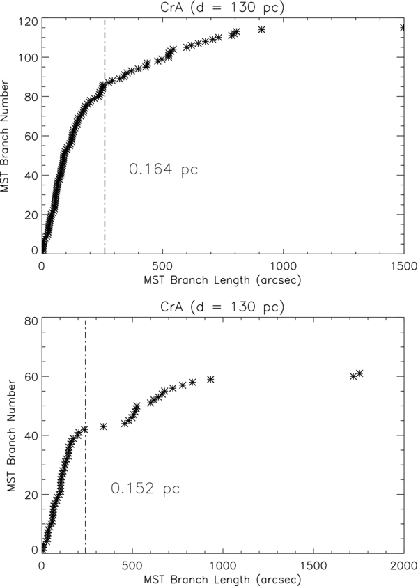
Figure 13. Upper panel: MST critical branch length for all 116 YSO candidates. Lower panel: MST critical branch length for the 62 Class I, Flat spectrum, and Class II sources (Class III sources are excluded).
Download figure:
Standard image High-resolution imageWe performed the same analysis for the 62 YSO candidates that had either Class I, Flat spectrum, or Class II SEDs (i.e., the Class III sources were excluded). Again, only one significant core was found, consisting of 34 members. The bottom panel of Figure 12 shows the MST of the YSO positions for these sources, and in this case, we obtained a Lcrit = 0.152 pc (see the bottom panel of Figure 13). Table 8 summarizes the results of this comparison, as well as the results of the Gutermuth et al. (2009) study, including values of Rcirc, Rhull, the aspect ratio R2circ/Rhull2, and the density for each core. For CrA, when looking at the core of 68 members, the value for Rcirc = 0.59 pc, with an aspect ratio of 2.36, indicating that the cluster is elongated. To illustrate this elongation, the convex hull for each grouping is shown (solid black line) in Figure 12.
Table 8. Clustering Analysis Comparison
| Cluster Properties | G09a | All YSO Candidates | Class I/II YSOs |
|---|---|---|---|
| (35 Sources) | (116 Sources) | (62 Sources) | |
| Lcrit | 0.116 pc | 0.164 pc | 0.152 pc |
| Ncores (no. of members) | 1 (24) | 1 (68) | 1 (34) |
| Rhull(core) | 0.200 pc | 0.385 pc | 0.237 pc |
| Rcirc(core) | 0.317 pc | 0.590 pc | 0.326 pc |
| Aspect ratiob | 2.51 | 2.36 | 1.89 |
| Densityc | 190 pc−2 | 150 pc−2 | 190 pc−2 |
Notes. aValues from Gutermuth et al. (2009). Note that they have been modified for a distance of 130 pc (a distance of 170 pc was used in their paper). bAspect Ratio = (Rcirc/Rhull)2. cDensity = Number of members in each core/(π × R2hull).
Download table as: ASCIITypeset image
The addition of new members from this paper changes the membership of the main CrA core from 24 members in the Gutermuth et al. (2009) study, to 68 members in our study of all classes of YSOs. However, the mean densities are quite similar since our analysis covers a larger area and includes known YSOs from the literature (see Table 8). In addition, the elongation of the core changes only slightly, from an aspect ratio of 2.51 to 2.36. A careful look at the differences in the top and bottom panels of Figure 12 shows that the Class III population extends further to the west, indicating an evolutionary stage gradient to the west in CrA. This confirms our qualitative analysis of Section 4.1, obtained from looking at the spatial distribution of YSOs (see also Figure 10), and the noted elongation of the CrA cloud from previous studies, as discussed in Section 1 (Neuhäuser et al. 2000; Mamajek & Feigelson 2001).
5. SUBMILLIMETER ANALYSIS
Six YSOs were detected in the dust continuum at 225 GHz by the SMA, and are listed with their flux densities in Table 9, and shown in Figures 14 and 15. The YSOs IRS 5, IRS 9, CXO 34, and CrA-24 were not detected above a 3σ rms level of 11 mJy (IRS 5) or 22 mJy (IRS 9, CXO 34, and CrA-24). The detected emission in all cases is compact and centrally concentrated, and is thus assumed to be primarily due to compact disk emission. Point source and two-dimensional Gaussian models were fitted to the detected YSOs, and for all sources but IRAS 32, the results were consistent with a point source, indicating unresolved emission on size scales of about 400 AU, consistent with disk sizes measured for other embedded YSOs (Jørgensen et al. 2007, 2009), and for T Tauri stars in nearby regions (Andrews & Williams 2007). For IRAS 32, an extended component is also present (more flux is recovered from fitting a Gaussian than from a point source alone), and is assumed to be due to inner envelope emission; this extended component was also seen in infrared imaging by Wilking et al. (1992). To remove this component, IRAS 32 was re-imaged using only baselines > 20 kλ, with the result being consistent with a point source. More detailed model fitting of IRAS 32, including two-dimensional radiative transfer, will be presented in a later paper. The flux densities reported in Table 9 are consistent with the values for SMA 2 (≡ RS 9) and SMA 1 (≡ IRS 7B) reported by Groppi et al. (2007), who observed with the SMA at a slightly higher frequency of ∼271 GHz.

Figure 14. SMA observations of the R CrA region. The image is the Spitzer 4.5 μm image. Two SMA mosaics are shown. On the right, indicated by the large dashed black circle, are the SMA observations of IRS 5 at 226 GHz. On the left, indicated by the large dashed oval-like shape, are SMA observations of the IRS 7 region at 224 GHz. The circle and oval, respectively, indicate the 50% sensitivity levels of the observations. In the IRS 5 region, the red contours indicate emission at the 6σ, 9σ,..., 18σ levels, where σ = 3.7 mJy beam−1 (46 × 26). In the IRS 7 region, the green contours indicate emission at the 3σ, 5σ, and 7σ levels,, while the yellow contours indicate emission at the 15σ, 27σ, and 39σ levels, where σ = 7.4 mJy beam−1 (55 × 23). Sources with black labels were detected by the SMA, while those with gray labels (in parentheses) were not. R CrA is detected at the 5σ level. The sources IRS 7B and SMA 2 (Radio Source 9; Brown 1987) are equivalent to SMA 1 and SMA 2 (Groppi et al. 2007, 271 GHz). The synthesized beams are shown as gray ovals at lower right (IRS 5) and lower left (IRS 7). Crosses indicate artifacts in the Spitzer data.
Download figure:
Standard image High-resolution image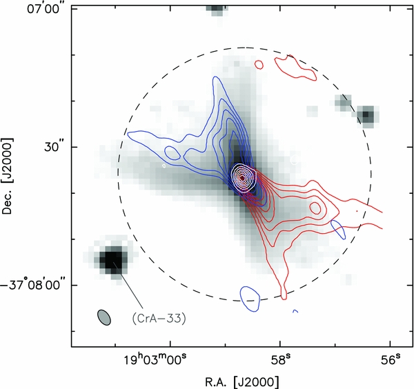
Figure 15. SMA observations of the CrA IRAS 32 region. The location of YSO candidate CrA-33 is also shown, although it was not detected with the SMA. The image is the Spitzer 4.5 μm image. The blue and red contours represent blueshifted and redshifted integrated 12CO 2–1 emission, respectively. The white contours represent 226 GHz continuum emission. Contour levels for the blueshifted and redshifted emission are 3σ, 6σ, etc., where 1σ = 1.0 Jy km s−1 and 0.7 Jy km s−1, respectively. The CO is integrated over local standard of rest velocities of [0,4.2] km s−1 and [6.7,11.6] km s−1 for blueshifted and redshifted emission, respectively. The contours of continuum emission are 3σ, 6σ, etc., where 1σ is 4.4 mJy beam−1. The large dashed circle shows the primary beam size of the SMA at 226 GHz, while the small gray oval at lower left shows the synthesized beam of 32 × 22.
Download figure:
Standard image High-resolution imageTable 9. Submillimeter Array Results
| Source | Other Name | R.A. (J2000)a | Decl. (J2000)a | F1.3 mmb,c | Mdiskd |
|---|---|---|---|---|---|
| (h m s) | (° ' '') | (mJy) | (M☉) | ||
| CrA-20 | IRS 5N | 19 01 48.47 | −36 57 14.9 | 95 (7) | 0.023 |
| R CrA | 19 01 53.65 | −36 57 08.6 | 36 (25) | 0.009 | |
| SMA 2 | 19 01 55.29 | −36 57 17.0 | 269 (20) | 0.063 | |
| IRS 7B | 19 01 56.40 | −36 57 28.3 | 320 (19) | 0.076 | |
| CrA-43 | WMB 55 | 19 01 58.52 | −36 57 09.3 | 135 (27) | 0.032 |
| CrA-44 | IRAS 32 | 19 02 58.68 | −37 07 36.7 | 103 (8) | 0.024 |
Notes. aR.A., decl. values from point-source fits to the continuum image data. bPoint-source fit to continuum images using baselines longer than 20 kλ. cThe uncertainties are reported in braces. These are the uncertainties returned by the fitting program IMFIT in MIRIAD. dDisk mass assuming a dust temperature of 30 K.
Download table as: ASCIITypeset image
If the disks are optically thin, the continuum fluxes provide a direct measure of the masses. For marginally optically thick emission, which is possible for such disks (Jørgensen et al. 2007; Andrews & Williams 2007), the mass becomes a lower limit to the true mass. The corrections are usually small, however. Previous studies of T Tauri stars (Andrews & Williams 2007; Lommen et al. 2007) indicate that the ratio of optically thick to thin emission is typically of order 0.2–0.3. This translates into an underestimation of the mass by up to a factor of two. Given the other assumptions (constant disk temperature, no radiative transfer modeling), this is a small correction. To compute disk masses, we use Equations (3) and (4) from Jørgensen et al. (2007) with their assumptions for the dust temperature (30 K) and 1.3 mm opacity (assuming a gas-to-dust ratio of 100). For the assumed distance of 130 pc for CrA, the disk mass at ∼225 GHz (1.3 mm) is
where F is the flux density measured in Jy. The results for the detected sources are listed in Table 9. The uncertainties listed in that table are those returned by the fitting procedure in MIRIAD, and are similar to the 3σ rms values reported earlier. So although the flux density of R CrA reported in this table is only 1.5 times the reported uncertainty, it is a well-detected source in the maps (about 5σ).
For the non-detected sources, the upper limits to the disk mass are 0.003 M☉ for IRS 5 and 0.005 M☉ for IRS 9, CrA-24, and CXO 34, that is, only a few Jupiter masses (MJ), and significantly less than the minimum mass solar nebula (MMSN), of 10–70 MJ (∼0.01–0.07 M☉; Weidenschilling 1977). In these cases, the masses are either very low, the dust has been processed into bodies significantly larger than a millimeter, and are thus mostly invisible to our observations (Lommen et al. 2007) or the dust is absent, perhaps due to clearing in a close binary (Jensen et al. 1996). It is known that IRS 5 is a close binary system (∼100 AU), and so this last scenario is a real possibility (see further discussion of IRS 5 in Appendix A.19; Chen & Graham 1993; Forbrich et al. 2006; Choi et al. 2008). The disk masses reported for the detected sources, aside from R CrA, are consistent with the MMSN.
The masses reported here are similar to masses of Class 0 and Class I protostars derived in an identical manner (0.017–0.089 M☉ and 0.009–0.076 M☉, respectively; Jørgensen et al. 2009). For Class II YSOs (T Tauri stars) also observed with the SMA, but analyzed with more detailed models, the masses are similar or slightly higher (0.003–0.18 M☉; Andrews & Williams 2007). The fluxes reported for the Class II YSOs are similar to those reported here (Andrews & Williams 2007), and lie at a similar distance (Taurus and Ophiuchus), so calculating masses using Equation (2) would produce masses similar to our results.
Observations at centimeter wavelengths show that the emission we have observed is most likely due to thermal dust emission, with essentially no contamination from free-free emission, except perhaps for R CrA (Choi et al. 2008; Miettinen et al. 2008). All sources, other than R CrA, are either weakly detected at cm wavelengths (<1 mJy), or not at all, with spectral indices between 4.9 and 8.5 GHz that are flat or negative. Although R CrA is also only weakly detected at cm wavelengths, it has a positive spectral index in the range 0.4–0.9, which implies that up to 5 mJy of the emission observed at 1.3 mm could be due to free-free emission, and so the disk mass should be slightly reduced to 0.008 M☉, which is consistent with the upper limit of 0.012 M☉ derived by Groppi et al. (2007).
6. OUTFLOWS AND JETS
6.1. Outflows and Jets Detected in H2 and Spitzer maps
Our H2 survey maps an area of about 20'×17', which spans from ∼5' east of the Coronet region to ∼4' west of S CrA, and from ∼3' north of TY CrA to ∼3' south of HH 101 (see Figure 4). The mapped region is about one-tenth of the Spitzer area, and is shown in Figure 16 as a green polygon on an IRAC/Spitzer three-color map of CrA.
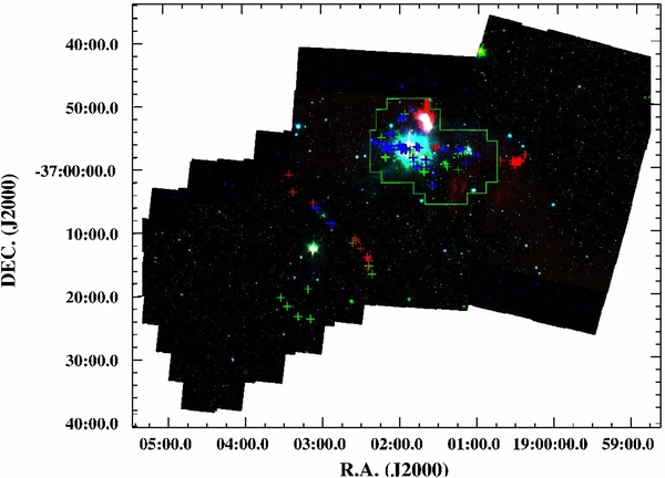
Figure 16. Spitzer three-color image of the CrA star-forming region, made from the IRAC 3.6 μm (blue), 4.5 μm (green), and 8 μm (red) images. The green polygon shows the area covered by our SofI H2 map. Green, blue, and red crosses indicate the position of HH objects, H2, and Spitzer knots, respectively.
Download figure:
Standard image High-resolution imageOur H2 continuum-subtracted mosaic reveals nearly 100 knots, some of them coincident with or close to previously known HH objects. These knots are shocked regions along the outflows, usually traced by H2 and/or Fe ii emission lines in the near-infrared (see, e.g., Caratti o Garatti et al. 2006), and ionic species in the optical (as O i, S ii, and Hα), also known as HH objects, which trace dissociative shocked regions with lower extinction and higher temperatures (see, e.g., Eislöffel et al. 1994). Once the continuum is removed from the H2 narrow-band images, what is left is the emission line alone, and thus knots and jets can be unambiguously identified. We detect 8 H2 counterparts out of 14 HH objects located in the mosaic FoV, while no evidence of molecular emission is observed from the remaining 6, namely HH 96, HH 729, HH 730, HH 734, HH 736, HH 860. Following Davis et al. (2010), we name the detected H2 flows MHO 2000–2014, followed by letters indicating knots and sub-structures inside each flow. It is worth noting that such a grouping is based on the flow morphology alone, and does not necessarily imply a real association to a single outflow. Davis et al. (2010) designated five MHOs (2000–2004) in the Coronet region, on the basis of morphology alone, because no P.M. analysis was available. Usually such a grouping is effective for isolated outflows and sources, where the outflows do not overlap and it is straightforward to recognize the outflow structure (chains of knots more or less aligned, bow-shocks indicating the outflow direction, etc.), which also points to the exciting source. On the other hand, it is often particularly difficult to disentangle different flows in crowded regions such as the Coronet, where several flows overlap, and the exciting sources are enclosed in a relatively small area. Here, we also use our P.M. analysis (see Section 6.2 and Appendix B) to recognize and group each flow. However, our analysis and thus our groupings are not resolute for several cases (see, e.g., Section 6.3 and Appendix B) due to the crowding in the Coronet and the uncertainties in our P.M. measurements. As a result, we keep the Davis et al. (2010) nomenclature, adding 10 more newly detected MHOs, i.e., MHO2005–2014, and include letters to pinpoint recognized knots and sub-structures within each MHO. We stress that such a grouping does not necessarily imply a real association to a single outflow.
The majority of the flows originate from the Coronet region and are radially distributed around it, with a larger concentration in the east and northeast regions (namely MHO 2000–2002, 2009, 2011–2014), and west and southwest regions (namely MHO 2003–2008), with MHO 2005 positioned around S CrA. Finally, MHO 2010 is positioned around IRAS 18595-3712 (IRAS 32). We identify about 14 H2 flows in CrA.
Most of the known HH objects, and all the detected H2 objects, are visible in our IRAC maps. Indeed, the IRAC maps contain molecular hydrogen lines that may be shock-excited in protostellar outflows (see, e.g., De Buizer & Vacca 2010, and references within). Generally, the H2 lines in band 2 (4.5 μm) and, partially, in band 1 (3.6 μm) have excitation conditions quite similar to the 1–0 S(1) line (2.12 μm), tracing shocks at T ∼ 2000 K (see, e.g., Caratti o Garatti et al. 2006; Takami et al. 2010). In particular, IRAC band 2 contains bright molecular hydrogen lines and can be used to detect knots (see, e.g., Cyganowski et al. 2008, 2009; Ybarra & Lada 2009), often called "extended green objects" (EGOs; Cyganowski et al. 2008), for the common coding of the 4.5 μm band as green in the IRAC three-color images. To better identify these features in the IRAC/Spitzer mosaics, we thus constructed IRAC three-color images, using 3.6 μm, 4.5 μm, and 8 μm (blue, green, and red, respectively, see Figure 16), and identified the new knots/EGOs by means of their colors and morphologies. Usually the outflow morphologies in band 2 and, partially, in band 1 resemble those observed in our H2 images, mostly delineating relatively high-excitation regions as bow shock heads or clumpy structures/knots along the flow axes. On the other hand, bands 4 and 3, which contain relatively low-excitation H2 lines, often delineate wings and wakes of bow shocks, and in general, milder shock regions (for a detailed analysis see Takami et al. 2010).
In addition to the H2 detected features, our Spitzer maps reveal three more flows positioned outside the H2 mosaic and named Spitzer outflow 1, 2, and IRAS 32 outflow, which include 30 additional new knots. Because we lack spectral confirmation, these flows could not be named MHO.
H2 and Spitzer newly detected knots and all previously known HH objects (including those not detected in H2) are labeled in our H2 map (see Figure 4) and in our three-color IRAC mosaic (Figure 16) as blue, red, and green crosses, respectively. Additionally, a list of known HH objects of the CrA star-forming region is reported in Table 10, and a complete list of knots detected in our Spitzer and H2 images is given in Table 11.
Table 10. Known HH Objects in CrA
| Knot | R.A. | Decl. | Knot | R.A. | Decl. |
|---|---|---|---|---|---|
| Name | (J2000) | (J2000) | Name | (J2000) | (J2000) |
| HH82A | 19 01 12.480 | −36 57 17.50 | HH729C | 19 01 15.679 | −36 57 56.41 |
| HH82B | 19 01 16.090 | −36 57 29.30 | HH730A | 19 01 25.26 | −36 59 30.0 |
| HH96 | 19 01 41.309 | −37 00 51.08 | HH730B | 19 01 24.079 | −36 59 59.78 |
| HH97 | 19 01 45.780 | −37 00 01.51 | HH730C | 19 01 15.720 | −37 00 29.99 |
| HH97E | 19 01 46.200 | −37 00 03.89 | HH731A | 19 01 40.030 | −36 58 57.29 |
| HH97W | 19 01 45.749 | −37 00 02.92 | HH731B | 19 01 38.270 | −36 58 45.59 |
| HH98 | 19 01 52.829 | −36 57 36.22 | HH732A | 19 01 57.199 | −36 52 07.21 |
| HH98B | 19 01 52.150 | −36 57 28.40 | HH732B | 19 01 56.410 | −36 51 38.41 |
| HH99 | 19 02 05.304 | −36 54 39.96 | HH732C | 19 01 57.730 | −36 52 17.00 |
| HH99A | 19 02 05.410 | −36 54 39.60 | HH733 | 19 02 09.470 | −36 54 46.19 |
| HH99B | 19 02 05.609 | −36 54 34.99 | HH734A | 19 02 11.011 | −36 58 28.60 |
| HH99C | 19 02 00.910 | −36 55 17.51 | HH734B | 19 02 11.729 | −36 58 22.69 |
| HH99E | 19 01 59.040 | −36 57 18.00 | HH735A | 19 02 12.559 | −36 56 37.79 |
| HH100 | 19 01 49.104 | −36 58 15.96 | HH735B | 19 02 12.761 | −36 56 42.11 |
| HH100N | 19 01 49.104 | −36 58 17.04 | HH736 | 19 02 14.410 | −36 55 22.19 |
| HH100S | 19 01 50.208 | −36 58 39.00 | HH860 | 19 01 39.401 | −36 58 03.79 |
| HH101 | 19 01 42.000 | −37 00 43.20 | HH861A | 19 02 21.569 | −37 16 54.98 |
| HH101N | 19 01 35.090 | −37 02 55.39 | HH861B | 19 02 24.300 | −37 15 38.02 |
| HH101S | 19 01 34.930 | −37 03 01.19 | HH862 | 19 02 36.581 | −37 11 57.19 |
| HH104 | 19 01 58.992 | −36 57 15.84 | HH863A | 19 03 09.010 | −37 23 55.72 |
| HH104D | 19 01 45.890 | −36 57 03.71 | HH863B | 19 03 10.819 | −37 19 12.29 |
| HH104C | 19 01 45.439 | −36 56 57.59 | HH863C | 19 03 18.600 | −37 23 31.20 |
| HH729A | 19 01 10.560 | −36 57 32.40 | HH863D | 19 03 26.909 | −37 21 54.40 |
| HH729B | 19 01 12.941 | −36 57 48.20 | HH863E | 19 03 31.699 | −37 20 32.60 |
Download table as: ASCIITypeset image
Table 11. Identified Knots in the CrA Star-forming Region
| Knot | R.A. | Decl. | Comments |
|---|---|---|---|
| Name | (J2000) | (J2000) | |
| Detected in IRAC maps—EGOs | |||
| Spitzer outflow 1 A | 19 00 24.139 | −36 58 07.20 | Part of a larger flow with outflow 2 and MHO 2005? |
| Spitzer outflow 1 B | 19 00 24.744 | −36 58 05.19 | Part of a larger flow with outflow 2 and MHO 2005? |
| Spitzer outflow 1 C | 19 00 27.379 | −36 59 00.99 | Part of a larger flow with outflow 2 and MHO 2005? |
| Spitzer outflow 1 D | 19 00 28.033 | −36 59 18.27 | Part of a larger flow with outflow 2 and MHO 2005? |
| Spitzer outflow 1 E | 19 00 28.304 | −36 58 53.48 | Part of a larger flow with outflow 2 and MHO 2005? |
| Spitzer outflow 1 F | 19 00 28.602 | −36 59 13.01 | Part of a larger flow with outflow 2 and MHO 2005? |
| Spitzer outflow 1 G | 19 00 29.218 | −36 59 00.20 | Part of a larger flow with outflow 2 and MHO 2005? |
| Spitzer outflow 1 H | 19 00 30.132 | −36 59 16.10 | Part of a larger flow with outflow 2 and MHO 2005? |
| Spitzer outflow 1 I | 19 00 30.648 | −36 59 01.46 | Part of a larger flow with outflow 2 and MHO 2005? |
| Spitzer outflow 1 J | 19 00 31.198 | −36 59 25.28 | Part of a larger flow with outflow 2 and MHO 2005? |
| Spitzer outflow 1 K | 19 00 31.308 | −36 59 08.80 | Part of a larger flow with outflow 2 and MHO 2005? |
| Spitzer outflow 1 L | 19 00 31.850 | −36 59 47.26 | Part of a larger flow with outflow 2 and MHO 2005? |
| Spitzer outflow 1 M | 19 00 31.962 | −36 59 30.18 | Part of a larger flow with outflow 2 and MHO 2005? |
| Spitzer outflow 1 N | 19 00 32.892 | −36 59 05.16 | Part of a larger flow with outflow 2 and MHO 2005? |
| Spitzer outflow 1 O | 19 00 33.592 | −36 59 32.03 | Part of a larger flow with outflow 2 and MHO 2005? |
| Spitzer outflow 1 P | 19 00 33.913 | −36 59 00.30 | Part of a larger flow with outflow 2 and MHO 2005? |
| Spitzer outflow 1 Q | 19 00 43.098 | −36 58 59.21 | Part of a larger flow with outflow 2 and MHO 2005? |
| Spitzer outflow 2 A | 19 01 31.574 | −36 57 03.69 | Jet-like morphology, part of MHO 2005 |
| Spitzer outflow 2 B | 19 01 32.635 | −36 56 55.58 | Jet-like morphology, part of MHO 2005 |
| Spitzer outflow 2 C | 19 01 34.272 | −36 56 56.71 | Jet-like morphology, part of MHO 2005 |
| IRAS 32 A | 19 03 25.207 | −37 01 07.39 | Part of IRAS 32 outflow—NE, blue lobe |
| IRAS 32 B | 19 03 22.159 | −37 03 53.27 | Part of IRAS 32 outflow—NE, blue lobe |
| IRAS 32 C | 19 03 06.643 | −37 05 33.85 | Part of IRAS 32 outflow—NE, blue lobe |
| IRAS 32 H | 19 02 34.231 | −37 11 19.14 | Part of IRAS 32 outflow—SW, red lobe |
| IRAS 32 I | 19 02 34.128 | −37 11 39.90 | Part of IRAS 32 outflow—SW, red lobe |
| IRAS 32 J | 19 02 30.290 | −37 12 46.61 | Part of IRAS 32 outflow—SW, red lobe |
| IRAS 32 K | 19 02 25.219 | −37 14 14.13 | Part of IRAS 32 outflow—SW, red lobe |
| IRAS 32 L | 19 02 24.948 | −37 14 20.23 | Part of IRAS 32 outflow—SW, red lobe |
| IRAS 32 M | 19 02 23.923 | −37 14 42.25 | Part of IRAS 32 outflow—SW, red lobe |
| IRAS 32 N | 19 02 24.840 | −37 16 05.23 | Part of IRAS 32 outflow—SW, red lobe |
| Detected in H2 and IRAC maps | |||
| IRAS 32 D | 19 03 04.142 | −37 06 21.01 | MHO 2010—Part of IRAS 32 outflow—NE, blue lobe |
| IRAS 32 E | 19 03 04.092 | −37 06 30.78 | MHO 2010—Part of IRAS 32 outflow—NE, blue lobe |
| IRAS 32 F | 19 02 53.472 | −37 08 47.56 | MHO 2010—Part of IRAS 32 outflow—SW, red lobe |
| IRAS 32 G | 19 02 51.478 | −37 09 01.72 | MHO 2010—Part of IRAS 32 outflow—SW, red lobe |
| MHO 2000 A | 19 02 05.561 | −36 54 37.60 | HH 99 B—Driven by IRS 9 or CrA 24 |
| MHO 2000 B | 19 02 04.668 | −36 54 56.40 | HH 99 A—Same flow of A? Possibly driven by IRS 6 |
| MHO 2001 A | 19 02 01.085 | −36 56 37.47 | Driven by CXO 34? |
| MHO 2001 B | 19 02 00.523 | −36 56 40.25 | Driven by CXO 34? |
| MHO 2001 C | 19 01 59.873 | −36 56 32.08 | Driven by YSO in the SMA 2 region |
| MHO 2001 D | 19 01 59.568 | −36 56 50.98 | Driven by CXO 34? |
| MHO 2001 E | 19 01 58.512 | −36 56 55.32 | Driven by CXO 34? |
| MHO 2001 F | 19 01 57.900 | −36 56 53.74 | Driven by YSO in the SMA 2 region |
| MHO 2001 G | 19 01 57.828 | −36 57 05.84 | Driven by CrA-43 (SMM 2) |
| MHO 2001 H | 19 01 57.660 | −36 56 59.79 | Driven by CrA-43 (SMM 2)? |
| MHO 2001 I | 19 01 56.626 | −36 56 57.79 | Driven by YSO in the SMA 2 region |
| MHO 2001 J | 19 01 56.412 | −36 57 17.09 | Driven by SMA 2? |
| MHO 2001 K | 19 01 56.110 | −36 57 02.84 | Driven by YSO in the SMA 2 region |
| MHO 2001 L | 19 01 55.792 | −36 57 11.62 | Driven by YSO in the SMA 2 region |
| MHO 2001 M | 19 01 55.475 | −36 57 18.80 | Driven by IRS 7A? |
| MHO 2001 N | 19 01 55.355 | −36 57 16.21 | Driven by SMA 2? |
| MHO 2001 O | 19 01 55.330 | −36 57 12.20 | Driven by YSO in the SMA 2 region |
| MHO 2001 P | 19 01 55.474 | −36 57 08.74 | Driven by YSO in the SMA 2 region |
| MHO 2001 Q | 19 01 52.520 | −36 57 16.12 | Driven by SMA 2? |
| MHO 2002 A | 19 01 59.462 | −36 57 17.63 | Driven by SMA 2? |
| MHO 2002 B | 19 01 59.222 | −36 57 14.46 | Driven by CrA-43 (SMM 2) |
| MHO 2002 C | 19 01 58.622 | −36 57 19.08 | Driven by SMA 2 or IRS 7B? |
| MHO 2003 A | 19 01 50.081 | −36 58 30.23 | Driven by IRS 1 |
| MHO 2003 B | 19 01 50.394 | −36 58 33.69 | Driven by IRS 1 |
| MHO 2003 C | 19 01 49.620 | −36 59 10.20 | Driven by IRS 1 |
| MHO 2004 A | 19 01 45.432 | −36 56 57.74 | HH 104C—bow-shock ∼east–west oriented—Part of a larger flow with MHO 2005? |
| MHO 2004 B | 19 01 45.864 | −36 57 03.79 | HH 104D—part of a curved jet ne-sw oriented. Driven by IRS 6 |
| MHO 2004 C | 19 01 46.849 | −36 56 53.99 | Part of a curved jet ne-sw oriented. Driven by IRS 6 |
| MHO 2004 D | 19 01 47.929 | −36 56 47.64 | Part of a curved jet ne-sw oriented. Driven by IRS 6 |
| MHO 2005 A | 19 01 28.879 | −36 57 10.66 | Part of a larger east–west flow? |
| MHO 2005 B | 19 01 25.702 | −36 57 21.11 | Part of a larger east–west flow? |
| MHO 2005 C | 19 01 16.202 | −36 57 28.73 | HH 82B - Part of a larger east–west flow? |
| MHO 2005 D | 19 01 15.790 | −36 57 26.35 | Part of a larger east–west flow? |
| MHO 2005 E | 19 01 12.038 | −36 57 08.52 | Part of a larger east–west flow? |
| MHO 2005 F | 19 01 09.670 | −36 59 23.75 | Part of a larger east–west flow? |
| MHO 2005 G | 19 01 04.706 | −36 58 09.74 | Part of a larger east–west flow? |
| MHO 2005 H | 19 01 12.426 | −36 57 17.09 | HH 82A—Part of a larger east–west flow? |
| MHO 2005 I | 19 00 59.969 | −36 58 15.00 | Part of a larger east–west flow? |
| MHO 2006 A | 19 01 40.923 | −36 58 47.18 | Driven by IRS 2 |
| MHO 2006 B | 19 01 40.827 | −36 58 52.08 | Driven by IRS 2 |
| MHO 2006 C | 19 01 40.033 | −36 58 57.85 | Driven by IRS 2 |
| MHO 2006 D | 19 01 33.924 | −37 01 03.54 | Driven by IRS 2 |
| MHO 2007 A | 19 01 34.937 | −37 02 55.89 | HH 101N—Driven by IRS 5? |
| MHO 2007 B | 19 01 34.282 | −37 03 01.41 | HH 101S—Driven by IRS 5? |
| MHO 2008 A | 19 01 47.393 | −36 59 52.30 | Part of a larger outflow incl. MH0 2003? |
| MHO 2008 B | 19 01 47.198 | −37 00 02.71 | Part of a larger outflow incl. MH0 2003? |
| MHO 2008 C | 19 01 46.214 | −37 00 05.50 | HH 97E—Part of a larger outflow incl. MH0 2003? |
| MHO 2008 D | 19 01 40.080 | −37 00 02.97 | Bow-shock ENE–WSW oriented, likely driven by CrA-41. |
| MHO 2009 A | 19 02 12.343 | −36 57 10.80 | Driven by SMA 2? |
| MHO 2009 B | 19 02 11.357 | −36 57 09.12 | Driven by SMA 2? |
| MHO 2009 C | 19 02 11.031 | −36 57 09.67 | Driven by SMA 2? |
| MHO 2009 D | 19 02 10.786 | −36 57 12.80 | Driven by SMA 2? |
| MHO 2009 E | 19 02 09.240 | −36 57 13.97 | Driven by SMA 2? |
| MHO 2009 F | 19 02 06.463 | −36 57 23.72 | Driven by SMA 2? |
| MHO 2009 G | 19 02 04.601 | −36 57 10.32 | Driven by SMA 2? |
| MHO 2011 A | 19 02 21.247 | −36 55 53.97 | Part of a large west–east precessing outflow |
| MHO 2011 B | 19 02 19.037 | −36 56 11.80 | Part of a large west–east precessing outflow |
| MHO 2011 C | 19 02 17.796 | −36 56 24.24 | Part of a large west–east precessing outflow |
| MHO 2011 D | 19 02 12.622 | −36 56 43.94 | HH 735B—Part of a large west–east precessing outflow |
| MHO 2011 E | 19 02 11.002 | −36 56 49.38 | Part of a large west–east precessing outflow |
| MHO 2011 F | 19 02 10.284 | −36 56 52.56 | Part of a large west–east precessing outflow |
| MHO 2012 A | 19 02 13.980 | −36 56 05.99 | Driven by IRS 7B? |
| MHO 2012 B | 19 02 07.356 | −36 56 36.37 | Driven by IRS 7B? |
| MHO 2012 C | 19 02 06.360 | −36 56 41.61 | Driven by IRS 7B? |
| MHO 2013 A | 19 02 09.447 | −36 54 41.50 | Driven by CXO 34? |
| MHO 2013 B | 19 02 09.454 | −36 54 49.02 | HH 733—Driven by CXO 34? |
| MHO 2013 C | 19 02 09.221 | −36 54 52.45 | Driven by CXO 34? |
| MHO 2014 A | 19 02 00.641 | −36 52 27.15 | Driven by IRS 5? |
| MHO 2014 B | 19 02 00.281 | −36 52 20.94 | Driven by IRS 5? |
| MHO 2014 C | 19 01 59.801 | −36 52 22.11 | HH 732C—Driven by IRS 5? |
| MHO 2014 D | 19 01 57.662 | −36 52 13.50 | Driven by IRS 5? |
| MHO 2014 E | 19 01 57.158 | −36 52 04.57 | HH 732A—Driven by IRS 5? |
| MHO 2014 F | 19 01 56.916 | −36 52 17.29 | Driven by IRS 5? |
In Appendices B, C, and D, a description of individual MHOs and Spitzer flows is given.
6.2. Proper Motions of H2 Knots
To derive P.M.s from our multi-epoch set of images, we followed the technique described in detail by Caratti o Garatti et al. (2009). As shown in Figure 4, the latest epoch map (SofI 2007) encloses all the remaining four; thus, we identify the SofI 2007 map as the common reference frame for our P.M. analysis. All earlier epoch maps were scaled and aligned to the reference frame with sub-pixel accuracy. The match was done using several field stars observed in each map (see Section 2.3), and optical distortions were corrected by means of the geomap (with a polynomial fit of third order) and geotran routines in IRAF. The resulting errors are represented by the residuals of the fits, and range between ∼0.2 and ∼0.4 pixels (i.e., ∼006–012), depending on the seeing and the number of stars in each map.
Knot shifts were determined between image pairs (i.e., last epoch and previous epoch maps) using a cross-correlation method. Knots were identified in the continuum-subtracted maps, and a rectangle was defined around each knot, enclosing its 3σ contour. The first epoch image was then shifted with respect to the last epoch image, with a sub-pixel accuracy of 0.1 pixel and then multiplied by it. For each shift (x, y), the total integrated flux (f) in the rectangle around each knot was measured in the product image. For the final shift for each knot, we used the position of the maximum of f(x,y), determined via a Gaussian fit.
Systematic errors for shift measurements were obtained by modifying the size and shape of the rectangle that defines each object. The resulting range of values gives a systematic error, which depends on the S/N, shape, and flux variability of the knot. This error is usually comparable to the alignment error. Thus, each single shift error was derived combining the alignment error of the two epoch images and the uncertainties in the centering routine. Usually, for each pair, the final error was around 20% of the P.M. value. It is worth noting that the number of P.M. measurements differs from knot to knot, depending on the number of matching maps. Thus knots located in the Coronet, with three or four P.M. measurements, usually have smaller errors.
In Figure 17, we show the flow charts of the CrA star-forming region. To display MHO motions for the entire region P.M.s, indicated by arrows, are reported in units of 500 yr. The results of our P.M. measurements are given in Table 12, which lists the knot ID, the measured P.M. in arcsec yr−1, the derived tangential velocity (vtan) in km s−1 at a distance of 130 pc, and the position angle (P.A.) in degrees of the P.M. vector. P.M.s were measured for knots observed in at least two different epochs. Moreover Table 12 reports only P.M.s with S/Ns larger than 2σ. As a result, 44 measurements are reported, namely those from MHO 2000, 2002, 2003, 2007, 2013, the majority of knots in MHO 2001, 2009, 2011, 2012, 2014, and some knots in MHO 2004, 2006, and 2008.
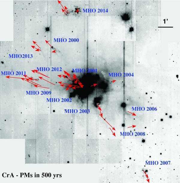
Figure 17. H2 flow chart of the CrA star-forming region. Proper motions in 500 yr are indicated by arrows.
Download figure:
Standard image High-resolution imageTable 12. Measured H2 Proper Motions in the CrA Knots
| Knot | P.M. | vtan | P.A. |
|---|---|---|---|
| Name | ('' yr−1) | (km s−1) | (°) |
| MHO 2000 A | 0.079 ± 0.009 | 49 ± 6 | 43 ± 6 |
| MHO 2000 B | 0.024 ± 0.007 | 15 ± 4 | 91 ± 16 |
| MHO 2001 A | 0.065 ± 0.007 | 40 ± 5 | 81 ± 5 |
| MHO 2001 B | 0.065 ± 0.007 | 40 ± 5 | 81 ± 5 |
| MHO 2001 C | 0.040 ± 0.010 | 24 ± 6 | 43 ± 15 |
| MHO 2001 D | 0.074 ± 0.010 | 46 ± 7 | 54 ± 8 |
| MHO 2001 E | 0.110 ± 0.010 | 70 ± 7 | 41 ± 5 |
| MHO 2001 F | 0.090 ± 0.015 | 55 ± 10 | 45 ± 10 |
| MHO 2001 G | 0.039 ± 0.007 | 24 ± 4 | 328 ± 10 |
| MHO 2001 J | 0.175 ± 0.006 | 108 ± 4 | 79 ± 2 |
| MHO 2001 K | 0.067 ± 0.009 | 41 ± 6 | 45 ± 8 |
| MHO 2001 M | 0.084 ± 0.018 | 52 ± 11 | 97 ± 8 |
| MHO 2001 N | 0.023 ± 0.009a | 14 ± 6a | 62 ± 23 |
| MHO 2001 O | 0.044 ± 0.012 | 27 ± 7 | 59 ± 14 |
| MHO 2001 P | 0.110 ± 0.010 | 70 ± 7 | 40 ± 5 |
| MHO 2001 Q | 0.058 ± 0.008 | 36 ± 5 | 289 ± 8 |
| MHO 2002 A | 0.083 ± 0.014 | 52 ± 9 | 81 ± 9 |
| MHO 2002 B | 0.056 ± 0.008 | 35 ± 5 | 133 ± 9 |
| MHO 2002 C | 0.040 ± 0.008 | 25 ± 5 | 65 ± 12 |
| MHO 2003 A | 0.110 ± 0.013 | 68 ± 8 | 199 ± 5 |
| MHO 2003 B | 0.056 ± 0.013 | 34 ± 8 | 220 ± 13 |
| MHO 2003 C | 0.186 ± 0.028 | 115 ± 17 | 225 ± 9 |
| MHO 2004 A | 0.038 ± 0.011 | 24 ± 7 | 286 ± 11 |
| MHO 2006 C | 0.075 ± 0.012 | 46 ± 8 | 243 ± 9 |
| MHO 2007 A | 0.073 ± 0.012 | 45 ± 8 | 215 ± 10 |
| MHO 2007 B | 0.097 ± 0.012 | 60 ± 8 | 201 ± 7 |
| MHO 2008 C | 0.085 ± 0.012 | 53 ± 7 | 215 ± 8 |
| MHO 2008 D | 0.071 ± 0.012 | 44 ± 8 | 261 ± 10 |
| MHO 2009 D | 0.147 ± 0.045 | 91 ± 28 | 63 ± 15 |
| MHO 2009 E | 0.137 ± 0.018 | 85 ± 11 | 66 ± 7 |
| MHO 2009 F | 0.127 ± 0.019 | 79 ± 12 | 80 ± 8 |
| MHO 2009 G | 0.147 ± 0.036 | 91 ± 22 | 63 ± 12 |
| MHO 2011 D | 0.068 ± 0.018 | 42 ± 11 | 68 ± 15 |
| MHO 2011 E | 0.256 ± 0.019 | 158 ± 12 | 84 ± 4 |
| MHO 2011 F | 0.080 ± 0.019 | 49 ± 12 | 76 ± 13 |
| MHO 2012 B | 0.134 ± 0.018 | 83 ± 11 | 68 ± 8 |
| MHO 2012 C | 0.140 ± 0.018 | 87 ± 11 | 62 ± 7 |
| MHO 2013 A | 0.086 ± 0.017 | 53 ± 11 | 45 ± 11 |
| MHO 2013 B | 0.041 ± 0.017a | 26 ± 11a | 101 ± 24 |
| MHO 2013 C | 0.091 ± 0.017 | 56 ± 11 | 63 ± 11 |
| MHO 2014 A | 0.065 ± 0.017 | 40 ± 11 | 32 ± 15 |
| MHO 2014 B | 0.133 ± 0.017 | 82 ± 11 | 34 ± 7 |
| MHO 2014 C | 0.071 ± 0.017 | 44 ± 11 | 31 ± 14 |
| MHO 2014 F | 0.037 ± 0.017a | 23 ± 11a | 347 ± 27 |
Download table as: ASCIITypeset image
The derived P.M. values range between 0.024 and 0.256 arcsec yr−1, corresponding to a vtan between 15 and 158 km s−1 (at a distance of 130 pc). The uncertainties vary from 0.006 to 0.045 arcsec yr−1 (i.e., ∼4 to ∼28 km s−1), depending on the knot S/N, the number of epochs, and the accuracy in the alignment. Such uncertainties, in turn, reflect on P.A. errors, which span from 2° to 27°.
A quick inspection of Figure 17 confirms that all the studied knots, except MHO 2008 D, are launched by YSOs inside or close to the Coronet. Several flows originate in the eastern part of the Coronet, in particular in a region a few arcseconds around SMA 2, which encloses several early stage YSOs (e.g., Nutter et al. 2005; Groppi et al. 2007).
A detailed analysis of P.M.s in single outflows is reported in Appendix B. There we show in more detail the flow charts of each region, where P.M.s (in 100 yr) and their error bars are indicated by arrows and ellipses, respectively (Figures 25–38).
Finally, a detailed discussion on outflow occurrence in CrA, and possible driving sources can be found in Section 6.3.
6.3. Outflows and Possible Driving Sources
Our H2 survey along with the Spitzer IRAC maps and P.M. analysis shows at least 14 different H2 flows in CrA. This number increases to 17 if we also include HH objects that do not have H2 counterparts but likely originate from one of the detected YSOs. However, the number of flows could be larger than this because we are not considering some of the HH objects which do not have a viable candidate driving source. Outflows and their possible driving sources were selected on the basis of the outflow morphology and P.M. analysis (see Section 6.1 and Appendix B). Candidate driving sources and their possible flows and position angles are reported in Table 13. Also blueshifted and redshifted lobes (hereafter blue and red lobes, respectively) have been tentatively indicated considering radial velocity measurements from this work (see Section 5 and Figure 15) and from the literature (Hartigan & Graham 1987; Levreault 1988; Anderson et al. 1997; Davis et al. 1999; Groppi et al. 2004, 2007; Knee 2005; van Kempen et al. 2009). Several question marks indicate the uncertainty in matching flows and sources. A clear match was obtained for those flows close to the driving source (IRS 1, IRS 2, IRS 6, SMM 2, SMA 2, IRS 7B, CrA-41), or driven by isolated YSOs (IRAS 32).
Table 13. Candidate Driving Sources and Possible Flows
| YSO | Flowa | P.A.(°)—Blue Lobe |
|---|---|---|
| IRS 1 | MHO 2003, MH0 2008 A–C (b) | 203 |
| IRS 2 | MHO 2006 (r?) | 26 |
| IRS 5N (?) | MHO 2007 (b); MH0 2014 (r) | 25 |
| IRS 6 | MHO 2000 B (?), HH 99 C (?) (r); MH0 2004 B–D (b?) | 240 |
| IRS 9 or CrA-24 | MHO 2000 A (r) | 229 or 223 |
| IRS 7A (?) | MHO 2001 F (?) | 55 |
| IRS 7B | MHO 2012, HH 736 (?), MHO 2002 C (r?); HH 731 B (?) (r?) | 248 |
| CXO 34 (?) | MHO 2013 (?), MHO 2001 A, B, E (?), F (?) (b?) | 45 |
| SMA 2 region | MHO 2013 (?), MHO 2001 O, P, K, I (?) (b?); MHO 2001 Q (r?) | ∼48 |
| SMA 2 | MHO 2009, MHO 2001 J, A (b?); MHO 2001 Q (r?) | 90 |
| IRS7 A or SMA 2 | MHO 2011 (b); MHO 2004 D; Sptz. outflow 1, 2, MHO 2005 (r) | ∼90 |
| CrA-43 (SMM 2) | MHO 2002 B, HH 734 (?) (b?); HH MHO 2001 G, H(?) (r?) | 125 |
| IRAS 32 | IRAS 32 outflow A–E (b); F–N, HH 861 (r) | 39 |
| CrA-41 | MH0 2008 D (b?) | 242 |
| CrA-40 (?) | HH 730 A–C (?) | 201 (?) |
| S CrA (?) | HH 762 (b?) | 115 |
| VV CrA (?) | HH 862 (b?) | 274 |
Note. ab = blue lobe, r = red lobe.
Download table as: ASCIITypeset image
The uncertainties in Table 13 are mainly due to the particular morphology of the Coronet region, as well as the uncertainties in the P.M. measurements. The majority of the flows originate from sources inside or close to the Coronet, in particular from the regions around SMA 2 and IRS 7A, where four known YSOs are located (namely SMA 2, IRS 7A, B, and CXO 34). However, we note that at least six different overlapping flows are launched from this region of the Coronet, likely indicating the presence of other embedded YSOs (see, e.g., Groppi et al. 2007; Choi et al. 2008; see also Figures 18 and 22). The overlap of the flows and the errors on the P.M.s do not allow us to pinpoint the driving sources, with the possible exceptions of SMA 2, IRS 7A, and IRS 7B, where the detected jets appear to be launched from or close to the positions of the sources (see Figures 22 and 23, and Appendix B). The SMA 2 flow should include MHO 2001 J, A; MHO 2009 to the east; and MHO 2001 Q to the west. The IRS 7B flow should include MHO 2002 C (see Figure 22), MHO 2012, possibly HH 736 in one lobe (see Figure 18), and possibly HH 731 B in the other lobe (see Figure 27 and Table 13).

Figure 18. SofI H2 image of the northeastern flows detected outside the Coronet.
Download figure:
Standard image High-resolution imageThere is also strong evidence of a very extended (∼1 pc) east–west wide precessing flow (∼15°), with blue and red lobes positioned east and west of the Coronet, respectively. This claim is also supported by CO observations from the literature (see, e.g., Knee 2005; Levreault 1988; Groppi et al. 2004, 2007). MHO 2011 matches well the CO blue lobe, whereas MHO 2004 D, Spitzer outflows 1 and 2, and MHO 2005 (see Figure 39) match the more extended CO red lobe. The driving source is likely to be one of the youngest sources in the region around SMA 2 and IRS 7A. SMA 2 would be the obvious candidate, but it already drives another jet, which is also east–west oriented, but with a smaller size and precession angle (∼4°; MHO 2002 and MHO 2009). However, we note that SMA 2 could harbor a binary or multiple system, as, e.g., reported by Choi et al. (2008). In this work, they detect three different sources, namely B9a/b in the centimeter continuum and CT 2 in the 7 mm continuum, positioned a few arcseconds north of IRS 7A, and at least two outflows (FPM 10 and FPM 13). We observe at least three different precessing flows escaping from the SMA 2–IRS 7A region (namely, knots MHO 2001 M, N, and O). Another possibility is that this large outflow is driven by IRS 7A.
Another large CO flow extends roughly south-southwest to north-northeast (Hartigan & Graham 1987; Levreault 1988; Anderson et al. 1997; Knee 2005), with HH 101 (MHO 2007) coincident with the blue lobe. HH 99 (MHO 2000) was previously believed to be the counterflow, but both geometric and kinematic considerations ruled out this hypothesis (see, e.g., Hartigan & Graham 1987; Davis et al. 1999). More recent CO observations (Knee 2005) place the peak of the red lobe far to the northwest, i.e., close to the position of the newly discovered MHO 2014, which is likely the counterflow, as both morphology and P.M. analysis also suggest. IRS 5 and 5N are positioned between the two lobes, thus one of the two is likely the driving source. Based on our SMA results, IRS 5N seems to be the most likely candidate, since no continuum emission from IRS 5 is detected (see also Section 5, Appendices A.19 and A.20).
There is no clear evidence of the HH 99 B (MHO 2000 A) counterflow in our analysis. The P.M. analysis indicates that MHO 2000 A and B (HH 99 B and A) are likely part of two distinct flows. MHO 2000 A could be driven by CrA-24, one of the newly discovered Class I YSOs, or by IRS 9 (see also Appendix B and Figure 18). MHO 2000 B seems to be part of a larger flow driven by IRS 6 (see also Appendices A and B, Figure 18, and Wang et al. 2004). Another Class I YSO, namely CrA-43 (or SMM 2) in the Coronet outskirts (see, e.g., Figures 14 and 22), is also driving an H2 outflow, southwest–northeast oriented (P.A. ∼125°), which includes MHO 2002 B, G, and possibly H, and HH 734 (see also Appendices A and B, and Wang et al. 2004).
On the basis of our morphological and kinematic analysis (see Appendix B), in Table 13 we tentatively associate the remaining observed H2 and HH objects with nearby detected YSOs. These possible matches are labeled in the table with a question mark. It is worth noting that we clearly detect only one lobe in several flows. Indeed this has already been observed in relatively crowded and confused regions (see, e.g., Davis et al. 2009), but our sample has an extremely high rate of single-lobe flows (9 out of 17), which is particularly disturbing. Although this can be ascribed to the morphology of the region, the high extinction (see Section 4.1), and the limited sensitivity of our survey, it could also indicate mismatches between flows and sources.
6.4. Incidence of Outflows versus Number and Class of YSOs
A more detailed analysis of Table 13 confirms that H2 outflows are mostly driven by early stage YSOs (see also Davis et al. 2009). Indeed, Class 0 source SMA 2 drives an H2 flow, as well as 10 out of the 14 YSO candidates classified as Class I. All of the Class I YSOs located near or in the Coronet seem to drive outflows. Three out of 43 Class II YSOs have H2 flows, which becomes 6 out of 43 Class II YSOs if we also consider flows with HH objects. None of the Class III sources shows any sign of outflow activity, indicating that accretion activity has reached completion in this stage, as one would expect. On the other hand, the percentage of H2 and atomic jets detected in Class II sources by this and previous surveys (e.g., Wang et al. 2004) seem to be too small (∼14%) for this class of objects because accretion should still be ongoing in Class II sources and thus outflows should be expected. This would then suggest that these surveys are not sensitive enough to detect such outflows or that there are mechanisms, for example, the cloud magnetic field, that inhibit the outflow activity in more evolved YSOs. Nevertheless, our data confirm that the accretion/ejection activity decreases with protostellar age. The H2 outflow sources are protostars (Class 0/I sources) rather than disk-excess sources (mostly Class II T Tauri stars), though a few of the latter source sample do seem to power H2 flows, and HH objects. However, if we exclude the IRS 6 flow, the H2 emission in these Class II flows is extremely reduced, whereas the HH and ionic emission are still well detected.
7. OVERALL CLOUD PROPERTIES
7.1. Disk Fraction
We have compiled a fairly complete estimate of the Class III population in CrA (see Section 3.5), and as a result, can examine the disk fraction of YSO candidates. There are 90 YSO candidates of all classes within the AV = 2 mag contours; of those, 42 are Class III YSO candidates. Therefore, the disk fraction in CrA is 53%. Recent disk fraction estimates for CrA include 53% by López Martí et al. (2010), who also included a population of diskless sources, and 67% by Meyer & Wilking (2009), who obtained the disk fraction from an extinction-limited sample of sources and used spectroscopic information to estimate an age range of 0.3–3 Myr from their H-R diagrams. Disk fraction values similar to ours have been inferred for young clusters NGC 7129 (54%; Gutermuth et al. 2004) and NGC 2264 (52%; Haisch et al. 2001). Based on comparison with theoretical PMS tracks, Haisch et al. (2001) estimate an age of ∼2.5 Myr for NGC 2264, which is consistent with the age range of 0.3–3 Myr estimated for CrA (Meyer & Wilking 2009).
7.2. Star Formation Rate and Efficiency
The mass of the CrA cloud can be estimated using the Spitzer + 2MASS extinction map discussed in Section 4.1. To compare our results to those for the c2d and GB clouds, we employ the same method used by Heiderman et al. (2010). They use the lowest resolution extinction map (FWHM = 270'') to calculate Mgas, cloud by summing up all the pixels (ΣAV) above an AV = 2 mag threshold, converting to column density using NH/AV = 1.37×1021 cm−2 mag−1 (Draine 2003) for a Weingartner & Draine (2001) RV = 5.5 extinction law, and obtaining Mgas, cloud = 279 M☉ (Heiderman et al. 2010). By following this procedure we obtain the same value for the cloud mass and the area of the cloud within the AV = 2 mag contour (i.e., 0.6 deg2), which translates to Acloud = 3.03 pc2 at a distance of 130 pc. By dividing Mgas, cloud by the area of the cloud, we obtain the average gas surface density of the cloud, Σgas, cloud = 92.1 M☉ pc−2. The range of gas surface densities for the c2d and GB clouds discussed in Heiderman et al. (2010) is Σgas, cloud ∼ 45–140 M☉ pc−2, and CrA falls in the middle of that range, similar to Chamaeleon I, Auriga, and Perseus.
Because we include additional YSO candidates not included in the Heiderman et al. (2010) study (i.e., NYSO, tot = 48 versus 41), the resulting star formation rate (SFR) for CrA is a factor of ∼1.2 higher than theirs. Note that only Class I, Flat spectrum, and Class II sources located in the area of the extinction map above the AV = 2 mag contours are considered. Following the analysis of Heiderman et al. (2010), we assume a mean YSO mass of 0.5 ± 0.1 M☉ over a period of star formation of 2 ± 1 Myr, based on estimates of the time span of the Class II phase (Evans et al. 2009). Using Equation (8) in Heiderman et al. (2010), we compute the SFR surface density to be ΣSFR = 3.96 M☉ yr−1 kpc−2, which translates to a SFR of 12.0 M☉ Myr−1. CrA has a relatively low SFR, compared with Perseus, Serpens, and Ophiuchus (96, 56, and 73 M☉ Myr−1, respectively; Evans et al. 2009; Heiderman et al. 2010), and is similar to the Lupus clouds, in particular Lupus III, Lupus V, and Lupus VI (17, 11, and 11 M☉ Myr−1, respectively; Heiderman et al. 2010). The SFR surface density, however, is the highest of all the clouds, with only Serpens showing similar values (ΣSFR = 3.29 M☉ yr−1 kpc−2; Heiderman et al. 2010). Similar comparisons were also made by Lada et al. (2010), where a useful graphical comparison of CrA with the c2d and GB clouds can be found (Lada et al. 2010, particularly, their Figures 2 and 4).
For comparison with the other c2d/GB regions, we also compute the star formation efficiency (SFE) for CrA using the following relation:
The total mass of the stars, M*, is estimated by multiplying the total number of stars (NYSO, tot = 48) by an assumed average stellar mass of 0.5 M☉. Using the entire cloud mass computed above (Mgas, cloud = 279 M☉), we obtain an SFE for CrA of ∼0.08. Evans et al. (2009) compiled SFE for several of the c2d clouds (see their Table 4), which range from 0.03 (Chamaeleon I) to 0.063 (Ophiuchus). The overall value of SFE for the GB cloud IC 5146 is ∼0.05 (Harvey et al. 2008). In general, CrA has the highest SFE of all the other clouds observed in c2d/GB surveys. This result is still valid even if we use the smaller, NYSO, tot = 41 value used in the Heiderman et al. (2010) study, so the effect is not merely a result of the addition of YSO candidates (although this may represent a useful measure of the uncertainties that the studies for the other c2d/GB regions may face due to incomplete YSO lists). Kirk et al. (2009) found an SFE of 8% for one of the GB regions, the Cepheus Flare region, when looking only at cores where groups of YSOs were located (and an SFE of 1% for the quiescent protostellar cores). In the case of CrA, perhaps we are seeing a small cloud of gas efficiently producing a cluster of stars and no additional regions of diffuse gas diluting the SFE.
The high SFE in CrA has been noted in the past (e.g., 45%, 40%, and 14%: Wilking et al. 1986; Harju et al. 1993; Tachihara et al. 2002, respectively). The very high estimate by both the Wilking et al. (1986) and Harju et al. (1993) studies is due to the fact that they used only the main Coronet core surrounding R CrA to estimate SFE (specifically, the area corresponding to the 2 μm survey by Taylor & Storey 1984). Wilking et al. (1992) compare the SFE of CrA with that of the ρ Ophiuchi cloud, which is similar in terms of distance and angular extent; also, neither cloud has a star more massive than B0V. They note that CrA has fewer YSOs than ρ Oph, and attribute that to the overall lower mass of both the low- and high-density molecular gas in the cloud (Dame et al. 1987; Loren 1979).
Tachihara et al. (2002) go a step further and compare the SFEs for a large sample of 179 cores in Taurus, the ρ Oph cloud, the Ophiuchus north region, the Lupus clouds, L1333, Southern Coalsack, the Pipe nebula, and CrA star-forming regions. They find an average SFE of roughly ∼10% for all the cores, with an SFE of 14% for all of CrA and 40% for the cluster-forming core of CrA. Using C18O observations, Tachihara et al. (2002) note that the regions with cluster-forming cores (in addition to CrA, this includes ρ Oph, Lupus III, and Chamaeleon I) have similar cloud structures, i.e., a head, where the active star formation occurs, and a tail that extends from it, suggesting that star formation has been triggered by an external shock. In order to explore this observation, they measure the average line widths, ΔV, for the starless cores which have not been disturbed by outflows from YSOs, and therefore represent the initial turbulent velocity in the cloud. The SFE, estimated using the total cloud mass from the 13CO clouds, is then plotted versus ΔV (see Figure 11 in Tachihara et al. 2002). For CrA, they estimate a cloud mass by applying the ratio of the total C18O core mass to the 13CO cloud mass to be 30%, and estimate SFE to be ∼4%.
In general, Tachihara et al. (2002) find that the regions actively forming stars, and whose 13CO-based SFE is greater than 2% (which includes CrA), all have ΔV < 0.7 km s−1 (conversely, the less active regions have ΔV > 0.7 km s−1). Based on these results, they suggest that a star-forming region with an initial turbulent velocity that is low will form stars spontaneously; if hit with a shock wave, the shock wave will then trigger the formation of a cluster in the head, forming a head–tail structure. Our observations and clustering analysis of CrA (see Section 4.2) are consistent with this picture: we see an elongated cluster core which is dominated by star formation in the "head," the Coronet, with a more extended population of PMS stars, and a quiescent clump in the southeastern "tail" of the cloud (Harju et al. 1993). As mentioned in Section 1, it has been shown that CrA is moving away from the Upper Centaurus Lupus (UCL) association with an expansion velocity similar to that of the Sco-Cen superbubbles (Mamajek & Feigelson 2001), specifically the H i shell of Loop I, suggesting that the expanding H i shell collided with the CrA cloud a few million years ago, triggering star formation in the Coronet, which is the part of the cloud facing the UCL (Harju et al. 1993). The "tail" of CrA is located downstream from the UCL association, which is also consistent with the triggering scenario.
8. SUMMARY
In this paper, we present the Spitzer Space Telescope, SMA, and H2 observations, combined with ROSAT and 2MASS, of the Corona Australis YSO population, its distribution, and outflows.
- 1.A total of 116 YSO candidates are identified, where 14 are classified as Class I, 5 are Flat spectrum, 43 are Class II, and 54 are Class III. These candidates were selected based on Spitzer, 2MASS, ROSAT, and Chandra observations, as well as an extensive search of the literature. Of the 116 YSO candidates, there are 12 which have not been selected as candidates by any previous study, where 3 are classified as Class I/Flat, 8 are Class II, and 1 is a Class III.
- 2.Six of these YSOs, R CrA, IRS 5N, IRS 7B, SMA 2 (RS 9), CrA-43 (SMM 2), and IRAS 32, were detected in the dust continuum at 225 GHz by the SMA. All sources except IRAS 32 have emission that is compact and centrally concentrated, assumed to be primarily due to compact disk emission. Disk masses for these sources were computed and range from 0.009–0.076 M☉. SMA data of IRAS 32 show an extended component, assumed to be due to inner envelope emission. The computed disk mass for IRAS 32 is 0.024 M☉.
- 3.An extinction map created using 2MASS and Spitzer data is presented and compared with the distribution of YSOs. The measured AV over the entire field has a mean of ∼5 mag, with a maximum of ∼30 mag, peaking on the Coronet. Using this extinction map, we calculated the cloud mass in the area of the extinction map above the AV = 2 contours to be 279 M☉, confirming the result found in Heiderman et al. (2010). There is a clear radial spread of sources from the Coronet, with Class I sources clustered most tightly in the center, surrounded by Class II sources. Class III sources can be found spread throughout the entire field.
- 4.We perform a clustering analysis mirroring that of Gutermuth et al. (2009), using the 116 YSO candidates identified in this paper, and confirm the Gutermuth et al. (2009) result that the CrA cluster is elongated (having an aspect ratio of 2.36) with a circular radius of 0.59 pc and mean surface density of 150 pc−2. By looking at the MST branches in the case where all YSOs are included compared with the case where the Class III sources have been excluded, it is clear that there is an evolutionary stage gradient in CrA, where the older Class III population extends to the west of the Coronet.
- 5.The star formation rate is calculated to be 12 M☉ Myr−1, similar to that of the Lupus clouds. The SFR surface density, however, is quite high: ΣSFR = 3.96 M☉ yr−1 kpc−2, similar to that of Serpens. A disk fraction is also calculated, and found to be 53% for CrA. The SFE for CrA is ∼8%, which is the highest of any of the c2d/GB regions surveyed, and is perhaps due to the triggering of star formation by an expanding H i shell associated with the Sco-Cen superbubbles.
- 6.Our H2 multi-epoch survey maps an area around CrA of about 20'×17' (i.e., ∼10% of the Spitzer map), and the continuum-subtracted mosaic reveals nearly 100 H2 knots, and we study P.M.s in 44 of them. The derived P.M. values range between 0.024 and 0256 yr−1, corresponding to a vtan between 15 and 158 km s−1 (at a distance of 130 pc).
- 7.We identify at least 17 outflows with their candidate driving sources. All the Class 0/I sources inside the Coronet, and the majority of Class I sources in the CrA region drive H2 flows. Most of the known HH objects, and all the detected H2 objects, are visible in our IRAC maps. Outflow morphologies in the 3.6 and 4.5 μm bands resemble those observed in our H2 images, mostly delineating relatively high-excitation regions, whereas the 5.8 and 8.0 μm bands mostly delineate wings and wakes of the bow shocks and, in general, milder shock regions.
- 8.There is clear evidence for a parsec-scale precessing outflow, E–W oriented, and originating in the SMA 2 region: IRS 7A or SMA 2 are likely the driving sources. Furthermore we likely identify the HH 101 lobe counterpart (MHO 2014), which is likely driven by IRS 5 or IRS 5N. By means of Spitzer mapping, we identify new flows in those regions not covered by our H2 maps: Spitzer outflows 1, and 2, which are likely part of the parsec-scale precessing outflow, E–W oriented, and the IRAS 32 outflow, which extends ∼0.8 pc and appears to precess as well.
The authors thank Karl Stapelfeldt, Eli Bressert, and the anonymous referee for their helpful comments. In addition, we thank Amanda Heiderman for very helpful discussions of the overall cloud properties and comparison with her work. Support for this work, part of the Spitzer Legacy Science Program, was provided by NASA through contract numbers 1288820 and 1298236 issued by the Jet Propulsion Laboratory, California Institute of Technology, under NASA contract 1407. A.C.G. was supported by the Science Foundation of Ireland, grant 07/RFP/PHYF790. The research at Centre for Star and Planet Formation (coauthor J.K.J.) is funded by the Danish National Research Foundation and the University of Copenhagen's programme of excellence.
This research is partially based on observations collected at the European Southern Observatory (Paranal and La Silla, Chile, 079.C-00020(A), 075.C-0561(A), 071.B-0274(A), 065.L-0637(A), 63.I-0031(A)). This research made use of APLpy, an open-source plotting package for Python hosted at http://aplpy.github.com. This research has also made use of NASA's Astrophysics Data System Bibliographic Services and the SIMBAD database, operated at the CDS, Strasbourg, France, and the 2MASS data, obtained as part of the Two Micron All Sky Survey, a joint project of the University of Massachusetts and the Infrared Processing and Analysis Center/California Institute of Technology, funded by the National Aeronautics and Space Administration and the National Science Foundation.
Facilities: Spitzer (IRAC, MIPS) - Spitzer Space Telescope satellite
APPENDIX A: NOTES ON INDIVIDUAL SPITZER-IDENTIFIED YSO CANDIDATES
In many cases, e.g., CrA-7, the ISOCAM source listed in Olofsson et al. (1999, hereafter O99) corresponds to one of our Spitzer YSO candidates, but is not exactly coincident with the position of the Spitzer detection. However, each case was checked and it was found that the ISOCAM sources listed as a match in this paper are within the pointing errors for both telescopes (and in no case is there another infrared source close enough to deem it questionable).
A.1. CrA-1
CrA-1 is too far afield to have been observed before; it is not included in the Forbrich & Preibisch (2007) Chandra study. CrA-1 is located in the western part of the CrA molecular cloud called "the streamer." It is not detected at 70 μm, but is bright at 24 μm; we classify it as a Class II, and it is a new YSO candidate.
A.2. CrA-2 (Leda Galaxy 90315)
CrA-2 was originally classified as a Class I YSO candidate from the Spitzer plus 2MASS photometry. However, by means of visual inspection, it proved to be a galaxy, and a quick search in SIMBAD found it to be Leda galaxy 90315. Interestingly, as was described in Section 3.2, another candidate YSO, CrA-50, is also included within the area which constitutes this extended source. Therefore, both CrA-2 and CrA-50 are clearly misclassified as YSO candidates and have been removed from our sample.
A.3. CrA-3 (ISO-CrA 55)
CrA-3 was detected with ISOCAM by O99, and is referred to as ISO-CrA 55 in their survey. From the ISOCAM photometry, it was found to have a mid-infrared excess, and therefore is listed as one of their YSO candidates.
Like CrA-1, it is located in "the streamer" so it has not been observed with Chandra. It is not detected at 70 μm, but is quite bright at 24 μm, and, according to Spitzer colors, has a Flat spectrum SED.
A.4. CrA-4 (DENIS-P J185950.9-370632, ISO-CrA 63)
CrA-4 is an association member, a young binary brown dwarf in CrA (Bouy et al. 2004). Known as DENIS-P J185950.9-370632, it was discovered to be a binary by Bouy et al. (2004) using high-resolution Hubble Space Telescope observations. The source was elongated in the WFPC2, ACS, and STIS images and the companion comes up clearly on the WFPC2 and ACS images after the primary PSF is subtracted. From the images, they found it to be a common P.M. pair with a separation of 0060. The magnitude difference between the two components indicates a mass ratio of ∼75%.
High- and low-resolution optical spectra of CrA-4 were also obtained, and the spectral features show that it is young, and likely an association member (Bouy et al. 2004). The high-resolution spectrum shows Hα in emission, and with a strength that makes it a likely accretor; there is also weak Li i absorption, which indicates a young age.
CrA-4 was detected with ISOCAM by O99, and is referred to as ISO-CrA 63 in their survey. It is not listed as a candidate YSO by O99 (i.e., it does not exhibit a mid-infrared color excess), however Bouy et al. (2004) analyzed the archival images and found there to be a mid-infrared excess in the 5.0–8.5 μm band. This is consistent with our Spitzer observations, which detect this source in all IRAC bands and at 24 μm, classifying it as a Class II YSO candidate based on the shape of its SED.
A.5. CrA-5 (ISO-CrA 76)
This source was detected with ISOCAM by O99, and is referred to as ISO-CrA 76 in their survey. From the ISOCAM photometry, it was found to have a mid-infrared excess, and therefore is listed as one of their YSO candidates.
CrA-5 is classified as a Class I YSO candidate by our method and is outside the Chandra FoV. Like CrA-1 and CrA-3, it is not detected at 70 μm, but is quite bright at 24 μm. Along with CrA-6 (Class II) and CrA-7 (Class III), these three YSO candidates surround "Spitzer outflow 1" which is discussed in more detail in Appendix D (see the upper right panel in Figure 39).
A.6. CrA-6 (CrAPMS 8, GP g2, ISO-CrA 88)
First observed in the infrared by Glass & Penston (1975), CrA-6 is listed as source [GP] g2 in their Table 1. It was also detected in X-rays by EINSTEIN, and its spectral type was estimated to be M3V (CrAPMS 8; Walter et al. 1997). Patten (1998) classifies it as a likely association member: he finds a spectral type of M5, and detects Hα in its spectrum, a ROSAT X-ray counterpart, and a VRI color excess.
Additionally, CrA-6 was detected with ISOCAM by O99, and is referred to as ISO-CrA 88 in their survey. From the ISOCAM photometry, it was found to have a mid-infrared excess, and therefore is listed as one of their YSO candidates. Most recently, it was one of the sources included in a kinematic study of the extended R CrA association (referred to as (GP75) R CrA g2 in their Table 13; Fernández et al. 2008), and found to be a member. All of this is consistent with our classification of CrA-6 as a Class II YSO candidate from its Spitzer photometry; we detect this source in all IRAC and MIPS bands out to and including 70 μm. Finally, CrA-6 was recently found to have a companion (Köhler et al. 2008).
A.7. CrA-7 (ISO-CrA 93)
CrA-7 was detected with ISOCAM by O99, and is referred to as ISO-CrA 93 in their survey. From the ISOCAM photometry, it was not found to have a mid-infrared excess. However, we classify CrA-7 as a Class III YSO candidate based on its Spitzer colors, and so it is a new YSO candidate. Bright 24 μm emission is detected, but nothing is detected at 70 μm.
A.8. CrA-8 (CrA-444)
YSO candidate CrA-8 was previously identified as a candidate low-mass member of CrA (López Martí et al. 2005, their source CrA-444) as part of their optical study of the very low mass population of CrA. Using a method outlined in López Martí et al. (2004), CrA-8 was classified from its optical spectrum as a brown dwarf candidate with spectral type of M8.5. We classify CrA-8 as a Class II YSO candidate from the shape of its SED, detecting it out to, and including, 24 μm.
López Martí et al. (2005) postulate that CrA-444 could have a very close companion, which they call CrA-444b. This source, approximately 23 away, is only visible in their deep I-band exposure. We do not see any conclusive evidence for CrA-444b in any of our Spitzer images, due to the lower spatial resolution.
A.9. CrA-9
CrA-9, located to the northwest of the Coronet region and TY CrA, has not been previously observed, thus it is a new YSO candidate, classified as a Class II. The source is located very close to the edge of the 70 μm map, so there is no catalog entry in this band for it. However, the MIPS 70 μm image clearly shows emission, and we estimate the flux using aperture photometry, finding a 70 μm flux of 154.2 ± 19.8 mJy (using a 2 pixel aperture radius).
A.10. CrA-10 (CrA-432)
López Martí et al. (2005) observed this source (referred to as CrA-432 in their Table 3) and found a photometric spectral type classification of M7 (one subclass error on the spectral type). Located near CrA-9, we classify CrA-10 as a Class II YSO candidate from the shape of its SED; it is detected in all bands out to, and including, 70 μm.
CrA-10 was also observed by Sicilia-Aguilar et al. (2008, also called CrA-432) with the Spitzer Infrared Spectrograph (IRS); the silicate feature at 8–13 μm is not detected in this source and there is only a marginal detection of the gas lines in the 13–14 μm IRS band.
Another identifier for this source is DENIS-P J190059.7-364711.
A.11. CrA-11 (HD 176269, HR 7169)
CrA-11, more commonly known as HD 176269, is an optically detected PMS star with a spectral type of B8V that was first observed by Knacke et al. (1973) as HR 7169 to be a possible member of the young stellar association near R CrA (∼12' to the SW). Another B8V star ∼12'' away, HR 7170 (HD 176270), was also listed as a possible member and we include it in Table 7. These two sources were detected, but not spatially resolved, by the IRAS (IRAS 18; Wilking et al. 1992) and EINSTEIN satellites (CrAPMS 10; Walter et al. 1997).
HD 176269 was observed in the near-infrared by Glass & Penston (1975) and is referred to in their Table 1 as source l; HD 176270 was also observed, and is listed as source k. Later, Patten (1998) does not classify the HD 176269/HD 176270 pair (which he calls source R05) as a likely association member: he finds a spectral type of B9V for the source and detects a ROSAT X-ray counterpart, however the source does not fulfill enough criteria for him to consider it an association member. Note that these stars are far enough afield so that they were not included as part of the Forbrich & Preibisch (2007) Chandra study.
HD 176269 was also detected with ISOCAM by O99, and is referred to as ISO-CrA 110 in their survey. ISO-CrA 110 was found to have a mid-infrared excess based on those observations so it is considered one of their YSO candidates. HD 176270 is referred to as ISO-CrA 111 in the same study, and it was not found to have a mid-infrared excess.
These studies are consistent with the Spitzer observations; we classify HD 176269 as a Class III based on the shape of its SED. Although we do not classify HD 176270 as a YSO candidate, it very likely is also a Class III based on its colors and SED shape (see Table 7). The SEDs of the two stars look similar out to 8 μm. However, at 24 μm, HD 176269 is much brighter than HD 176270. Neither source is detected at 70 μm.
A.12. CrA-12 (V667 CrA, CrA-4110)
CrA-12 (or V667 CrA; Kukarkin et al. 1972) is a known variable star, detected with Chandra (J190116.26-365628.4; Forbrich & Preibisch 2007) and with ISOCAM (ISO-CrA 123; O99). CrA-12 was not found to have a mid-infrared excess based on the ISOCAM observations. However, based on our Spitzer observations, it is classified as a Class II YSO candidate. It does not have a 70 μm detection, but is quite bright at 24 μm.
López Martí et al. (2005) observed this source (referred to as CrA-4110 in their Table 3) and found a photometric spectral type classification of M5 (error of two subclasses on the spectral type). The same spectral classification was also obtained by Sicilia-Aguilar et al. (2008), who classify it as a weak-line T Tauri star (wTTs), due to its small Hα equivalent width (EW) and the fact that it has no other accretion indicators (see their Table 5). A Spitzer IRS spectrum was obtained for CrA-12 but only a short-low (5–14 μm) spectrum was extracted; the silicate feature from 8–13 μm was not detected in this source (Sicilia-Aguilar et al. 2008).
Another identifier for this source is DENIS-P J190116.3-365628.
A.13. CrA-13 (CrA-466)
CrA-13 is likely ISO-CrA 127 (O99), which is slightly offset (∼11'') from the CrA-13 Spitzer coordinates. ISO-CrA 127 does fall within the extent of the very bright 24 μm source, though, so it is highly likely this is the same source. We detect CrA-13 in all IRAC bands and in both the 24 and 70 μm MIPS bands, and classify it as a Class II from its SED. This source was also detected with Chandra (J190118.90-365828.4; Forbrich & Preibisch 2007).
López Martí et al. (2005) observed this source (referred to as CrA-466 in their Table 3) and found a photometric spectral type classification of M4.5 (error of two subclasses on the spectral type). However, Sicilia-Aguilar et al. (2008), who also obtained an optical spectrum, classified it as an M2 based on the strength of its spectral features. Moreover they identify it as a classical T Tauri star (cTTs) because it has strong Hα emission (see their Table 5; it is also referred to as CrA-466 in their paper). They also classify CrA-13 as a transition object (TO) due to its lack of infrared excess at wavelengths shorter than 6 μm. However, Ercolano et al. (2009) run several models to fit the SED of the source using the spectral type of M2 given by Sicilia-Aguilar et al. (2008), and find that its SED is well fit by an untruncated disk model, and is likely not a TO. Recent SED modeling performed by Currie & Sicilia-Aguilar (2011) confirms the Ercolano et al. (2009) conclusion, identifying it as an optically thick primordial disk. A Spitzer IRS spectrum was obtained for CrA-13 and shows silicate emission in both the 8–13 μm and 20–30 μm regions (Sicilia-Aguilar et al. 2008).
Another identifier for this source is DENIS-P J190118.9-365828.
A.14. CrA-14 (HH 101 IRS 1, G-94)
CrA-14 is an infrared source first observed by Reipurth & Wamsteker (1983) to be associated with HH 101, and they call it IRS 1. HH 101 was observed again, in the optical, by Hartigan & Lada (1985) who called it HH 101 7.
This source was also detected with ISOCAM by O99, and is referred to as ISO-CrA 137 in their survey. ISO-CrA 137 was not found to have a mid-infrared excess based on those observations. This is consistent with our Spitzer observations which classify this source as a Class III YSO candidate based on its SED; it is faint at 24 μm and not detected at 70 μm. This source was also detected with Chandra (J190129.01-370148.8; Forbrich & Preibisch 2007), making it a likely YSO candidate. It was observed in multiple epochs with Chandra and was found to have some variable X-ray emission as well as enhanced activity in one of the epochs (Forbrich et al. 2007).
CrA-14 was also observed by Sicilia-Aguilar et al. (2008), which they call G-94, who obtained an optical spectrum and classified it as M3.5 based on its spectral features. They classify it as wTTs due to its small Hα EW and the fact that it has no other accretion indicators (see their Table 5). A Spitzer IRS spectrum was obtained for G-94, but no silicate emission was seen (Sicilia-Aguilar et al. 2008).
Another identifier for this source is DENIS-P J190129.0-370148.
A.15. CrA-15 (IRS 14)
CrA-15 was first observed by Taylor & Storey (1984, hereafter TS84), and called IRS 14 (TS 2.9), with the 3.9 m Anglo-Australian Telescope, using its infrared photometer–spectrometer system. This same source was observed with increasingly better arrays in the near-infrared by Wilking et al. (1986) and later Wilking et al. (1997, source 185809.8-370224). However, each time, IRS 14 was classified as a field star due to its lack of a near-infrared excess. Based on Spitzer photometry, we classify IRS 14 as a Class II YSO candidate; it is not detected at 70 μm but its detection at 24 μm gives it a mid-infrared excess consistent with a Class II SED. O99 saw this mid-infrared excess as well (their source ISO-CrA 139, see their Table 1) and therefore also considered it a YSO candidate. IRS 14 was detected with Chandra (J190132.34-365803.1; Forbrich & Preibisch 2007).
IRS 14 was also observed by Sicilia-Aguilar et al. (2008), which they call G-87, who obtained an optical spectrum and classified it as M3−M4 based on the strength of its spectral features compared with other, known M stars. They classify it as wTTs due to its small Hα EW and the fact that it has no other accretion indicators (see their Table 5). They also classify IRS 14 as a TO due to its lack of infrared excess at wavelengths shorter than 6 μm. However, as was discussed in Appendix A.13 for CrA-13, Ercolano et al. (2009) found that the SED for IRS 14 was also well fit by an untruncated disk model, and is likely not a TO. Recent SED modeling performed by Currie & Sicilia-Aguilar (2011), though, includes Spitzer IRAC 8 μm photometry (not included by Ercolano et al. 2009), and finds that the best-fit model for IRS 14 is that of a depleted transitional disk. A Spitzer IRS spectrum was obtained for IRS 14 and shows silicate emission in the 8–13 μm region as well as marginal detections of gas lines in the 13–14 μm region (Sicilia-Aguilar et al. 2008).
Another identifier for this source is DENIS-P J190132.2-365803.
A.16. CrA-16 (IRS 13)
CrA-16 was also observed by TS84, and is known as IRS 13 (TS 2.8). Like IRS 14, this source was observed with increasingly better arrays in the near-infrared by Wilking et al. (1986), and later Wilking et al. (1997, source 185811.4-370206). Unlike IRS 14, though, a near-infrared excess was seen for IRS 13 and so it was considered a cTTs and association member. IRS 13 was also detected with Chandra (J190133.84-365745.0; Forbrich & Preibisch 2007).
IRS 13 and IRS 14 are about 30'' apart, and CrA-17 (discussed in the next section) is just a little bit further away. Based on Spitzer photometry, we classify IRS 13 as a Class II YSO candidate; it is not detected at 70 μm but its detection at 24 μm gives it a mid-infrared excess consistent with a Class II SED. An optical spectrum was obtained by Sicilia-Aguilar et al. (2008), who refer to IRS 13 as G-85, and classify it as M2−M3 based on the strength of its spectral features compared with other, known M stars; it also has strong Hα emission, confirming it as a cTTs (see their Table 5). A Spitzer IRS spectrum was obtained, and as for CrA-13, shows silicate emission in both the 8–13 μm and 20–30 μm regions (Sicilia-Aguilar et al. 2008).
A.17. CrA-17
CrA-17 was first observed in the near-infrared by Wilking et al. (185813.8-370225; 1997). Based on the Spitzer catalog, we classify CrA-17 as a Class II YSO candidate. The catalog lists a 24 μm flux for CrA-17, but that flux was obtained by band-filling, and after examining the images, it appears that the detection may not be real. In addition, although CrA-17 falls within the region covered by the Forbrich & Preibisch (2007) Chandra study, it is not detected in X-rays. Due to these reasons, we have removed CrA-17 from our list of candidate YSOs.
A.18. CrA-18 (G-65)
CrA-18 is located just north of TY CrA (see Figure 21), and was first observed in the near-infrared by Wilking et al. (1997, source 185818.2-365603). Based on Spitzer photometry we classify CrA-18 as a Class II YSO candidate; it is not detected at 70 μm but its detection at 24 μm gives it a mid-infrared excess consistent with a Class II SED. This source was also detected with Chandra (J190140.40-365142.4; Forbrich & Preibisch 2007).
An optical spectrum was obtained by Sicilia-Aguilar et al. (2008), who refer to CrA-18 as G-65, and classify the source as M1−M2 based on the strength of its spectral features compared with other, known M stars; it also has strong Hα emission, confirming it as a cTTs (see their Table 5). Also, as was discussed in Appendices A.13 and A.15 for CrA-13 and IRS 14, Ercolano et al. (2009) found that the SED for CrA-18 was also well fit by an untruncated disk model, and is likely not a TO. Recent SED modeling performed by Currie & Sicilia-Aguilar (2011) confirms the Ercolano et al. (2009) conclusion, identifying it as an optically thick primordial disk. A Spitzer IRS spectrum was obtained for CrA-18, but no silicate emission was seen (Sicilia-Aguilar et al. 2008).
A.19. CrA-19 (IRS 5, MMS 12, SMM 4)
Best known as IRS 5, this was one of the first infrared sources to be associated with CrA (TS 2.4; Taylor & Storey 1984). IRS 5 was first seen to be a binary by Chen & Graham (1993), and later confirmed by Nisini et al. (2005), who found a separation of ∼78 AU between the two components (at a distance of 130 pc). Nisini et al. (2005) also found a spectral type for IRS 5A of K5−K7V (IRS 5B was too faint to classify). Additionally, IRS 5 was detected with the VLA at 6 cm (called VLA 7; Brown 1987), and shows significant short- and long-term variability in the radio (Suters et al. 1996). Feigelson et al. (1998) detected circularly polarized continuum emission at centimeter wavelengths in IRS 5, demonstrating that radio emission from protostars can sometimes arise from non-thermal processes. IRS 5 is also a millimeter source, MMS 12 (Chini et al. 2003), and was observed at 450 and 850 μm by Nutter et al. (2005, referred to in their survey as SMM 4), seen as an extended source in their maps. Using photometry available in the literature at the time, Chen et al. (1997) use a distance of 130 pc to estimate Tbol = 403 K and Lbol = 0.9 L☉ for IRS 5 (which they refer to as TS 2.4 in their Table 2).
The Chandra X-ray emission for the binary is only marginally resolved, so IRS 5A/B is listed as a single source in the catalog of Forbrich & Preibisch (2007, J190148.02-365722.4). However, a later study by Hamaguchi et al. (2008) used a subpixel repositioning technique in order to resolve the X-ray emission from multiple Chandra observations. They found that IRS 5A is flaring, while IRS 5B is quiescent. IRS 5A/B is also resolved by Choi et al. (2008), called CHLT 3 (IRS 5A) and CHLT 4 (IRS 5B), in their centimeter imaging survey of CrA.
With Spitzer, we classify IRS 5 as a Class I YSO candidate; it is detected in all bands out to, and including, 24 μm. We do not resolve the binary. In addition, IRS 5 is one of the sources which we observed with the SMA (see Section 5), and surprisingly, there is no clear detection, although IRS 5N does show strong detection (see Figure 14 and Appendix A.20).
A.20. CrA-20 (IRS 5N)
IRS 5N was first seen in the radio (Forbrich et al. 2006, listed as source 5), and then later in X-rays with Chandra, and referred to as IRS 5N (J190148.46-365714.5; Forbrich & Preibisch 2007; Forbrich et al. 2007). Based on Spitzer photometry, we classify IRS 5N as a Class I YSO candidate; it is detected in all bands out to and including 24 μm. IRS 5N was one of the sources we observed with the SMA, and it has a strong detection (see Section 5 and Figure 14). We compute a disk mass for IRS 5N of 0.023 M☉ (see Table 9).
A.21. CrA-21 (IRS 8)
CrA-21 was also observed by TS84, and is known as IRS 8 (TS 2.2). Like IRS 13 and IRS 14, this source was observed with increasingly better arrays in the near-infrared by Wilking et al. (1986), and later Wilking et al. (1997, source 185828.8-365834). Unlike IRS 14, though, a near-infrared excess was seen for IRS 8 and so it was considered an association member. We classify CrA-21 as a Class II YSO candidate; it is not detected at 70 μm but its detection at 24 μm gives it a mid-infrared excess consistent with a Class II SED.
Meyer & Wilking (2009) also classify this source as a likely association member from H- and K-band spectra, finding it to be consistent with a G5 star. Additionally, it was detected with Chandra (J190151.11-365412.5; Forbrich & Preibisch 2007).
A.22. CrA-22
CrA-22, which is located directly south of the Coronet, is too far afield to have been observed before, nor is it included in the Forbrich & Preibisch (2007) Chandra study. Another source falls very close to CrA-22 in the IRAC bands, however, the catalog flux detections of CrA-22 are good, and do not appear to contaminate the photometry. CrA-22 has a MIPS detection at 24 μm, but is not detected at 70 μm. We classify CrA-22 as a Class II, and it is a new YSO candidate.
A.23. CrA-23 (Star A)
First detected by Graham (1993), CrA-23, referred to as "Star A" (which was not detected by IRAS), was found to be very bright in Hα, weaker in the R-band, and very weak (only just visible) in the original S ii image. They recognized it as a likely strong emission-line star, but it was too faint to obtain a spectrum.
Later, Star A was also detected in the infrared J, H, K' bands by Wilking et al. (1997, source 185831.1-370456), who classified it as a brown dwarf candidate. López Martí et al. (2005) found a photometric spectral type classification of M8.5 (1 subclass error on the spectral type) for Star A (they call it CrA-465). Sicilia-Aguilar et al. (2008) obtained an optical spectrum (also referred to in their paper as CrA-465), classifying it as M7.5 based on the strength of its spectral features; it also has strong Hα emission which is double peaked, confirming it as a cTTs (see their Table 5). With Spitzer, we detect Star A in all IRAC bands and at 24 μm, but not at 70 μm. We classify it as a Class II YSO candidate based on its SED.
Another identifier for Star A is DENIS-P J190153.7-370033.
A.24. CrA-24
We classify CrA-24 as a Class I YSO candidate based on its Spitzer SED. It is definitely detected up through 8 μm with a rising SED, however, it is difficult to tell whether or not the 24 μm MIPS detection is an actual detection due to contamination from the nearby R CrA nebula. It is not detected in our SMA data (see Figure 14), but it is observed by Chandra (J190155.61-365651.1; Forbrich & Preibisch 2007). Due to its position, CrA-24 could be a good candidate driving source for HH 99 (MHO 2000 A; see Figure 18). Thus, we include it as a new YSO candidate.
A.25. CrA-25
CrA-25 is classified as a Class I YSO candidate based on its Spitzer SED, but that SED is based on almost all band-filled fluxes. Looking at CrA-25, it is clear that it is an extended source, a knot that is associated with an HH object, located within 3'' of HH732A (Wang et al. 2004). Therefore, CrA-25 has been removed from our list of candidate YSOs.
A.26. CrA-26 (WMB 185844.2-370304)
CrA-26 was detected by Wilking et al. (1997) in the infrared J, H, K' bands (named 185844.2-370304). It is classified with Spitzer as a Class II YSO candidate and is well detected through 8 μm. There is a flux listed at 24 μm, but it is suspect due to the fact that it falls within a diffraction spike; the 24 μm flux has been band-filled. After inspecting the SED (see Figure 7), we determine that it looks like a YSO candidate out to and including 8 μm. Therefore, we retain CrA-26 as a candidate Class II YSO.
A.27. CrA-27 (WMB 185848.1-365808)
CrA-27 was detected by Wilking et al. (1997) in the infrared J, H, K' bands (named 185848.1-365808). Also detected by O99 (ISO-CrA 142), it did not exhibit a mid-infrared color excess and was not listed as a candidate YSO. However, Meyer & Wilking (2009) obtained an infrared spectrum and determined it to be a likely association member, "late-type" > K4. With Spitzer, we classify CrA-27 as a Class III YSO candidate, which is consistent with the other studies.
A.28. CrA-28 (ISO-CrA 143, G-14)
CrA-28 was detected by Wilking et al. (1997) in the infrared J, H, K' bands (named 185849.3-370733). It was also detected with ISOCAM by O99 (ISO-CrA 143), was found to have a mid-infrared excess, and therefore is listed as one of their YSO candidates. CrA-28 is similar to CrA-30 (see Appendix A.30) because they both have small H−K colors and similar SEDs (O99). On the basis of our Spitzer data, we classify this source as a Class II YSO candidate; it is detected out to and including 24 μm. CrA-28 also has a Chandra detection (J190211.99-370309.4; Forbrich & Preibisch 2007).
This source was also observed by Sicilia-Aguilar et al. (2008), called G-14, who obtained an optical spectrum and classified it as an M4.5 based on the strength of its spectral features. They classify it as wTTs because it has weak/no Hα emission (see their Table 5). They also classify it as a TO due to its lack of infrared excess at wavelengths shorter than 6 μm. However, Ercolano et al. (2009) run several models to fit the SED of G-14 using the spectral type of M4.5 given by Sicilia-Aguilar et al. (2008), and find that its SED is well fit by an untruncated disk model, and is likely not a TO. Recent SED modeling performed by Currie & Sicilia-Aguilar (2011), though, includes Spitzer IRAC 8 μm photometry (not included by Ercolano et al. 2009), and finds that the best-fit model for IRS 14 is that of a depleted transitional disk. A Spitzer IRS spectrum was obtained and it shows silicate emission in the 8–13 μm region (Sicilia-Aguilar et al. 2008).
A.29. CrA-29 (ISO-CrA 145)
CrA-29 was detected by Wilking et al. (1997) in the infrared J, H, K' bands (named 185852.0-370456). It was also detected with ISOCAM by O99 (ISO-CrA 145), was found to have a mid-infrared excess, and therefore is listed as one of their YSO candidates. With Spitzer, we classify this source as a Class II YSO candidate, and it is detected out to and including 24 μm.
A.30. CrA-30 (Hα 14; HBC 680)
CrA-30 was detected as an emission-line star by Marraco & Rydgren (1981, Hα 14) and is also listed in the Herbig & Bell Catalog as HBC 680 (Herbig & Bell 1988). It has also been noted as an IRAS detection, source IRAS 18591-3702, (e.g., Weintraub 1990; Wilking et al. 1992). Using photometry available in the literature at the time, Chen et al. (1997) use a distance of 130 pc to estimate Tbol = 2604 K and Lbol = 1.2 L☉ for Hα 14.
This source was detected by Wilking et al. (1997) in the infrared J, H, K' bands (named 185904.3-370238), and by O99 (ISO-CrA 155). From the ISOCAM photometry, it was found to have a mid-infrared excess, and therefore is listed as one of their YSO candidates. Hα 14 has a Chandra detection (J190227.05-365813.2; Forbrich & Preibisch 2007), and in addition, it was found to have a companion (Köhler et al. 2008). A Spitzer IRS spectrum was obtained, and the source, referred to as G-1, shows silicate emission at 8–13 μm (Sicilia-Aguilar et al. 2008).
Most recently, Hα 14 was one of the sources included in a kinematic study of the extended R CrA association (Fernández et al. 2008, referred to as HBC 680 in their Table 13), and found to be a member; it was also observed by Meyer & Wilking (2009) and determined from its infrared spectrum to be an M0 member of the association. All of these observations are consistent with our Spitzer observations which show it to be well detected out to and including 24 μm, classifying it as a Class II YSO candidate from its SED.
A.31. CrA-31 (Hα 3, ISO-CrA 159)
CrA-31 is an emission-line star of M type (Marraco & Rydgren 1981, Hα 3). Chen et al. (1997) use a distance of 130 pc to estimate Tbol = 1875 K and Lbol = 0.6 L☉ for Hα 3. This source was also detected with ISOCAM by O99 (ISO-CrA 159), was found to have a mid-infrared excess, and therefore is listed as one of their YSO candidates. In addition, it was detected with Chandra (Forbrich & Preibisch 2007, catalog number J190233.07-365821.1). Our Spitzer observations classify this source as a Class II YSO candidate and it is detected all the way out to and including 70 μm.
A.32. CrA-32
We originally classified CrA-32 as a Flat spectrum YSO candidate based on its Spitzer SED. However, its MIPS 24 μm flux has been band-filled and is likely not very accurate due to the fact that CrA-32 is close to the very bright 24 μm source, CrA-44 (also known as IRAS 32; see Appendix A.44). In the IRAC bands, there is also another source in very close proximity, making CrA-32 look quite extended. Due to the complicated nature of this source, CrA-32 has been removed from our list of candidate YSOs.
A.33. CrA-33 (IRAS 32d)
CrA-33 is classified as a Flat spectrum YSO candidate based on its Spitzer SED, and is well detected out to and including 24 μm. It was first observed by Wilking et al. (1992) as part of the IRAS 32 outflow, and is referred by to them as IRAS 32d. It was also detected with ISOCAM by O99, and is referred to as ISO-CrA 185 in their survey. From the ISOCAM photometry, it was found to have a mid-infrared excess, and therefore is listed as one of their YSO candidates. Located to the southeast of the main IRAS 32 outflow (see Figures 15 and 40), CrA-33 is too far afield to have been observed by many other surveys, e.g., it is not included in the Forbrich & Preibisch (2007) Chandra study.
A.34. CrA-34 (ISO-CrA 198)
This source was detected with ISOCAM by O99, and is referred to as ISO-CrA 198 in their survey. From the ISOCAM photometry, it was found to have a mid-infrared excess, and therefore is listed as one of their YSO candidates.
Located to the north of IRAS 32, CrA-34 is too far afield to have been observed by many other surveys, e.g., it is not included in the Forbrich & Preibisch (2007) Chandra study. Based on the shape of its Spitzer + 2MASS SED, we classify it as a Class III YSO candidate and it is detected in all bands up to and including 24 μm.
A.35. CrA-35 (ISO-CrA 201)
This source was detected with ISOCAM by O99, and is referred to as ISO-CrA 201 in their survey. From the ISOCAM photometry, it was found to have a mid-infrared excess, and therefore is listed as one of their YSO candidates.
Located very close to IRAS 32, just to the southeast, CrA-35 is too far afield to have been observed by many other surveys, e.g., it is not included in the Forbrich & Preibisch (2007) Chandra study. Based on the shape of its Spitzer + 2MASS SED, we classify it as a Class II YSO candidate and it is detected in all bands up to and including 24 μm.
A.36. CrA-36
Also located to the southeast of IRAS 32, CrA-36 is too far afield to have been observed by many other surveys, e.g., it is not included in the Forbrich & Preibisch (2007) Chandra study. Based on the shape of its Spitzer + 2MASS SED, we classify it as a Class II YSO candidate and it is detected in all bands up to and including 70 μm. CrA-36 has not been classified as a YSO candidate before; therefore it is a new YSO candidate.
A.37. CrA-37
CrA-37 was possibly detected with ISOCAM by O99, and referred to as ISO-CrA 232 in their survey. ISO-CrA 232 is ∼8'' away from CrA-37 which is close to the pointing uncertainties for both telescopes; there are no other infrared sources nearby so it is likely that this is the same source. From the ISOCAM photometry, ISO-CrA 232 was not found to have a mid-infrared excess, and therefore is not listed as one of their YSO candidates.
CrA-37 is too far afield to have been observed by many other surveys, e.g., it is not included in the Forbrich & Preibisch (2007) Chandra study. It is located to the southeast of IRAS 32. Based on the shape of its SED, we classify it as a Class I YSO candidate and it is detected in all bands up to and including 70 μm. CrA-37 has not been classified as a YSO candidate before; therefore it is a new YSO candidate.
A.38. CrA-38 (ISO-CrA 13)
CrA-38 was detected with ISOCAM by O99, and is referred to as ISO-CrA 13 in their survey. From the ISOCAM photometry, it was found to have a mid-infrared excess, and therefore is listed as one of their YSO candidates.
CrA-38 is also too far afield to have been observed by many other surveys, e.g., it is not included in the Forbrich & Preibisch (2007) Chandra study. Like CrA-1 and CrA-3, it is located in the western part of the CrA molecular cloud, "the streamer." Based on the shape of its Spitzer + 2MASS SED, we classify it as a Class III YSO candidate and it is detected in all bands up to and including 24 μm.
A.39. CrA-39 (6dFGS gJ190023.5-371224)
CrA-39 was originally classified as a Class II YSO candidate from the Spitzer + 2MASS photometry. However, a closer look at the images reveals that it is a galaxy (indicated in SIMBAD to be an emission-line galaxy, 6dFGS gJ190023.5-371224). Therefore, this source is clearly misclassified as a YSO candidate and has been removed from our sample.
A.40. CrA-40 (VSSt 18, ISO-CrA 134)
CrA-40 was first observed at 2.2 μm by Vrba et al. (1976a, known as VSSt 18) and later by Wilking et al. (1997) in the infrared J, H, K' bands (named 185802.9-370344). CrA-40 was also detected with ISOCAM by O99, and is referred to as ISO-CrA 134 in their survey. From the ISOCAM photometry, it was found to have a mid-infrared excess, and therefore is listed as one of their YSO candidates. Additionally, it was detected with Chandra (J190125.75-365919.3; Forbrich & Preibisch 2007).
Most recently, CrA-40 was classified by Meyer & Wilking (2009) from its infrared spectrum as a K3 member of the association. All of this is consistent with our Spitzer observations, which detect this source in all IRAC bands and at 24 μm, classifying it as a Class II YSO candidate.
A.41. CrA-41 (Hα 2, HBC 677)
CrA-41 is an emission-line star, first observed by Marraco & Rydgren (1981, Hα 2), and listed in the Herbig & Bell Catalog as HBC 677 (Herbig & Bell 1988). This infrared source is known to be a part of HH 100, which was observed in the optical by Hartigan & Lada (1985) who called it HH 100 1, and was detected by Wilking et al. (1997) in the infrared J, H, K' bands (named 185819.1-370418). CrA-41 also has a Chandra detection (J190141.62-365953.1; Forbrich & Preibisch 2007).
Most recently, CrA-41 was one of the sources included in a kinematic study of the extended R CrA association (referred to as HBC 677 in their Table 13; Fernández et al. 2008), and found to be a member; it was also classified by Meyer & Wilking (2009) from its infrared spectrum as an M2 member of the association. All of these observations are consistent with our Spitzer observations, which detect this source in all IRAC bands and at 24 μm, classifying it as a Class II YSO candidate based on the shape of its SED.
A.42. CrA-42 (IRS 6)
CrA-42 is a binary source, known as IRS 6A and 6B, first noted as a binary by Nisini et al. (2005); we do not resolve it in our Spitzer images. Nisini et al. (2005) found a separation of 97 AU (<1'') between the two components (at a distance of 130 pc), and a spectral type for IRS 6A of M2V (IRS 6B was too faint to classify). Positionally, our YSO candidate CrA-42 is closer to the coordinates given by Nisini et al. (2005) for IRS 6A, but we will discuss both IRS 6A and 6B here (referring to it as "IRS 6," since it is unresolved in most studies).
IRS 6 was first observed by TS84 (TS 2.3), and then by Wilking et al. (1986), and later Wilking et al. (1997, source 185828.2-370058). Using photometry available in the literature at the time, Chen et al. (1997) use a distance of 130 pc to estimate Tbol = 1055 K and Lbol = 0.1 L☉ for IRS 6 (which they refer to as TS 2.3 in their Table 5).
Along with several Class I sources in the Coronet cluster (including IRS 1, IRS 2, IRS 5, IRS 7, IRS 9, and R CrA), IRS 6 was first seen in X-rays by Koyama et al. (1996) with the ASCA satellite. Interestingly, it was not detected in X-rays with ROSAT (Neuhäuser & Preibisch 1997), although the ROSAT band has a softer energy range than ASCA. Forbrich et al. (2006) find that IRS 6 is detected as a weak X-ray source with Chandra and XMM-Newton, and is referred to as IRS 6A in Table 2 of Forbrich & Preibisch (source J190150.45-365638.1; 2007)
Wilking et al. (1997) noted that IRS 6 is associated with a reflection nebula, and Wang et al. (2004) infer that it could be the driving source for a giant outflow including HH objects HH 99, 730, 860, and the HH 104 D jet (see Figure 28). However, Caratti o Garatti et al. (2006) discount IRS 6 as the driving source for HH 99 based on the tangential velocity and position angle of HH 99 (see their Section 7.11 and their Figure 15). On the basis of our analysis, we suggest that IRS 6 is driving a large outflow that includes MHO 2000 B, HH 99 C, and MH0 2004 B–D (see also Appendix B and Table 13).
In the radio, IRS 6 has been seen as a very weak source at 3.6 cm and 6 cm (Forbrich et al. 2006; Miettinen et al. 2008). Unlike IRS 5A/B, IRS 6A/B was not resolved by Choi et al. (2008) in their centimeter imaging survey of CrA, in which they refer to IRS 6 as CHLT 5. In fact, like the previous studies, the single source is only weakly detected in their 3.5 cm continuum map, and flux values for densities at both 6.2 and 3.5 cm are not listed in their Table 3.
Most recently, IRS 6 was classified by Meyer & Wilking (2009) from its infrared spectrum as an M1 member of the association. All of these observations are consistent with our Spitzer observations, which detect this source in all bands up to and including 24 μm, and classify it as a Class II YSO candidate.
A.43. CrA-43 (SMM 2, CHLT 15, WMB 55)
CrA-43 was first observed by Wilking et al. (1997) in the infrared J, H, K' bands (named 185836.1-370131). This source corresponds to SMM 2 from the Nutter et al. (2005) SCUBA 450 and 850 μm survey of CrA. Nutter et al. (2005) also refer to the near-infrared counterpart of SMM 2 as WMB 55 because it is source number 55 in Table 1 of Wilking et al. (1997). Groppi et al. (2007) mention this source within their study of SMA observations of the IRS 7 region (of which SMM 2 is nearby), however, their field did not cover the SMM 2 region. Although CrA-43 is part of the field covered by Chandra, it is not detected (Forbrich & Preibisch 2007).
In Haas et al. (2008), CrA-43 is identified as a candidate YSO using a millimeter excess technique, called A3 51, with a 1.2 mm flux of 101.8 ± 18.4 MJy sr−1. It is also weakly detected in 3.5 cm continuum emission by Choi et al. (referred to as CHLT 15; 2008), but not in the 6.2 cm continuum. A close-up of CrA-43 and the surrounding flows can be seen in Figures 22 and 23, as well as in Figure 5 ([S ii] narrow-band images) of Wang et al. (2004), clearly indicating that it is driving an outflow (see also Appendix B and Table 13).
In our Spitzer images, CrA-43 is well detected out to and including 24 μm and is classified as a Class I YSO candidate. It is also detected with the SMA (see Figure 14), and we compute a disk mass for CrA-43 of 0.032 M☉ (see Table 9).
A.44. CrA-44 (IRAS 32c)
CrA-44 is classified as a Class I YSO candidate based on its Spitzer SED, and is well detected out to and including 160 μm. It was first observed by Wilking et al. (1992) as part of the IRAS 32 outflow and is referred to by them as IRAS 32c (IRAS 18595-3712). Using photometry available in the literature at the time, Chen et al. (1997) use a distance of 130 pc to estimate Tbol = 148 K and Lbol = 1.3 L☉ for IRAS 32 (see their Table 2). It was also detected with ISOCAM by O99, and is referred to as ISO-CrA 182 in their survey. From the ISOCAM photometry, it was found to have a mid-infrared excess, and therefore is listed as one of their YSO candidates. IRAS 32 has a near-infrared reflection nebula first reported by Connelley et al. (2007), and named the "Isabelle-Nebula" by Haas et al. (2008), which they observed in the H and Ks bands. This reflection nebula can be easily seen in the infrared Spitzer bands and ISAAC/VLT narrow-band 2.12 μm image, and it likely delineates the outflow cavity (see Figure 40).
There have been other Spitzer studies of IRAS 32 as well. Seale & Looney (2008) show that the outflow cavity has an opening angle averaging 66° ± 4. Because IRAS 32 is nearly edge-on, when correcting for inclination angle, Seale & Looney (2008) find a similar average opening angle of 65° ± 4. In addition, a Spitzer IRS spectrum of IRAS 32 shows a solid CH4 feature at 7.7 μm (Öberg et al. 2008).
IRAS 32 is also a millimeter source, MMS 23 (Chini et al. 2003), and was observed at 450 and 850 μm by Nutter et al. (2005, referred to in their survey as SMM 8). Using the Atacama Pathfinder Experiment, van Kempen et al. (2009) observed IRAS 32 in the submillimeter lines of CO, HCO+ and their isotopologues, finding it to be a truly embedded source with an exceptionally strong outflow. This is confirmed by our SMA, H2, and Spitzer observations (see Section 5, Appendix B, and Figure 15), which show a parsec-scale precessing outflow. Using the SMA data, we compute a disk mass for IRAS 32 of 0.024 M☉ (see Table 9).
IRAS 32 is too far afield to have been observed by many other surveys, e.g., it is not included in the Forbrich & Preibisch (2007) Chandra study.
A.45. CrA-45 (VSSt 10, IRAS 34)
CrA-45 was first observed at 2.2 μm by Vrba et al. (1976a, known as VSSt 10), and is an IRAS source, named IRAS 34 by Wilking et al. (1992). Using photometry available in the literature at the time, Chen et al. (1997) use a distance of 130 pc to estimate Tbol = 712 K and Lbol = 0.5 L☉ for VSSt 10 (see their Table 2).
Located to the southeast of IRAS 32 (CrA-44), CrA-45 is on the outskirts of the main CrA cloud core, and is the closest YSO candidate to the quiescent "Core C" discussed in Harju et al. (1993) at about ∼8' to the northwest. It is too far afield to have been observed by many other surveys, e.g., it is not included in the Forbrich & Preibisch (2007) Chandra study. Our Spitzer observations classify CrA-45 as a Class II YSO candidate, and it is well observed out to and including 70 μm.
APPENDIX B: NOTES ON INDIVIDUAL MHOs—NORTH AND EAST REGIONS, CORONET
B.1. Morphology
Figure 18 shows a SofI H2 image of northeastern flows detected outside and inside the Coronet. We observe at least seven H2 flows radially launched from the Coronet. The well known MHO 2000 A (i.e., HH 99 B, see, e.g., Davis et al. 1999; Caratti o Garatti et al. 2006); MHO 2000 B (i.e., HH 99 A); MHO 2013 (i.e., HH 733, see Wilking et al. 1997; Davis et al. 1999; Wang et al. 2004); and four newly detected outflows, namely, MHO 2009, 2011–2014. MHO 2011, and 2014, are partially coincident with HH 733 and 732 (see Wang et al. 2004), respectively. Finally, MHO 2001 and 2002 (Caratti o Garatti et al. 2006; Davis et al. 2010), positioned inside the Coronet are labeled with blue crosses in Figure 18.
A close-up view of MHO 2009, 2011, and 2012 is given in Figure 19. MHO 2009 is composed of a chain of precessing knots (A–F), roughly elongated west–east for ∼12. About 20'' northward, MHO 2011 (knots A-G) shows a curved shape, elongated toward east-northeast, and is more extended (∼36). Knots D and F are the brightest structures. The first is a large bow-shock, coincident with HH 735, while the second has a point-like shape.
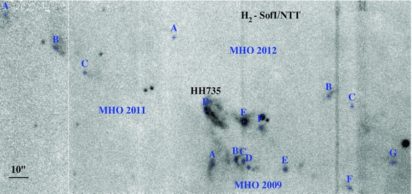
Figure 19. Close-up view of MHOs 2009, 2011, and 2012 at 2.12 μm, from a SofI/NTT image (see Figure 18). Labels and crosses indicate names and positions of detected knots and sub-structures along the flows.
Download figure:
Standard image High-resolution imageRoughly 25'' northward, we detect three faint aligned knots (MHO 2011 A–C) oriented southwest–northeast (length ∼17). HH 736, not detected in our H2 images, is positioned farther northeastward, and although not well aligned with the knots, could be part of the flow. Further north (see Figure 18) we detect MHO 2013 and 2000, molecular counterparts to HH 733 and HH 99. A close-up view of the two flows is given in Figure 20. Both flows are roughly parallel and elongated toward the northeast. MHO 2013 shows a morphology identical to the [S ii] emission observed by Wang et al. (2004), with three brighter condensations located at the curved head of the jet. MHO 2000 is composed of two bright structures, a heading bow-shock (A - HH 99 B) and a knot (B - HH 99 A), with a rough bow-shape, oriented toward MHO 2013. It is not clear whether or not this last is associated with the main flow or with the MHO 2013 flow, although our P.M. analysis marginally indicates that the latter is the case (see Appendix B.2 and Figure 25).
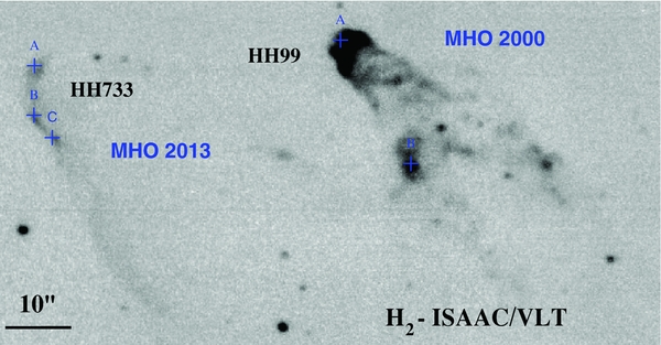
Figure 20. Close-up view of MHOs 2000 and 2013 at 2.12 μm, from a ISAAC/VLT image (see Figure 18). Labels and crosses indicate names and positions of detected knots and sub-structures along the flows.
Download figure:
Standard image High-resolution imageAbout 5' northward of the Coronet and ∼35 to the east of TY CrA, we discover MHO 2014, the brightest MHO in CrA (see Figure 18). The MHO extends for roughly 1', and displays an extremely complex morphology, as shown in Figure 21, where H2 and H2 continuum-subtracted images are reported. Three arc-shaped structures are visible in the eastern part of the object (knots A–C), while the brightest knots (D–F) are located in the western part, partially coincident with HH 732 A and C. Such a puzzling structure could be caused by the interaction of several bow-shocks from a precessing flow or the overlapping of different flows. Notably, HH 732 B, not detected in H2, is located ∼30'' to the north, suggesting that more than one flow could be present.
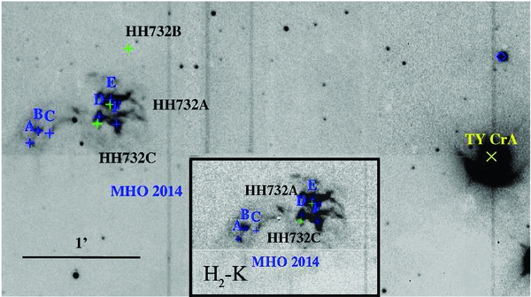
Figure 21. Close-up view of MHOs 2014 at 2.12 μm, from a SofI/NTT image (see Figure 18). Labels and crosses indicate names and positions of detected knots and sub-structures along the flows.
Download figure:
Standard image High-resolution imageFlow detection and P.M. study inside the Coronet region is particularly difficult, due to the presence of R CrA and the extremely bright and diffuse nebulosity around it, which cannot be completely removed in our H2 continuum-subtracted images (see, e.g., Figure 22, upper panel). Several H2 knots east and northeast of R CrA and around CrA-43 (SMM 2) (see, e.g., Nutter et al. 2005; Groppi et al. 2007) were previously discovered by Caratti o Garatti et al. (2006) and named MHO 2001 and 2002 by Davis et al. (2010). Figure 22 (upper panel) shows a SofI H2 continuum-subtracted image of the region, where we detect more knots positioned a few arcseconds northeast and east of the SMA 2 and IRS 7A region (see, e.g., Groppi et al. 2007). Following Davis et al. (2010), the new knots are named MHO 2001 from K to Q, although it is clear that MHO 2001 and 2002 consist of several overlapping flows. Knot Q is the only source of H2 emission detected westward of R CrA. MHO 2001 is an elongated chain of scattered knots (roughly directed southwest–northeast), with several knots grouped around the SMA 2 and IRS 7A regions, which are the focal point of several flows. A closer look with ISAAC/VLT is given in Figure 22 (lower panel). The H2 image is shown in logarithmic scale to display simultaneously the bright regions close to SMA and the fainter knots of MHO 2002. Unfortunately, an ISAAC H2 continuum-subtracted image is not available for this region. The ISAAC/VLT image reveals the presence of at least five different flows in this region, possibly more. Knots C, I, K, P, O are possibly part of a first flow directed north-northeast (displayed with white arrows). A second flow could consist of MHO 2001 A–E, L, N, directed northeast (cyan arrows). MHO 2002 A is the terminal bow-shock of a third outflow (roughly west–east oriented, P.A.∼90°) delineated by green arrows in the figure. It is not clear whether MHO 2002 C could be part of this flow, or, as a faint H2 trail seems to suggest could be driven by IRS 7B (yellow arrows). MHO 2001 J is the jet of MHO 2002 A, and knot M could be part of the flow as well (green arrows). This flow matches well the centimeter maps by Choi et al. (2008), who detected a west–east jet launched by SMA 2. This is also observed in the CO 3–2 maps by van Kempen et al. (2009), who detected a west–east flow (P.A.∼ 90°). The blue lobe is positioned to the east of SMA 2 region, while the red lobe is to the west. Another flow (red arrows), southeast–northwest oriented (P.A.∼125°), and composed of MHO 2002 B, MHO 2001 G, and possibly H, seems to originate from CrA-43 (SMM 2).
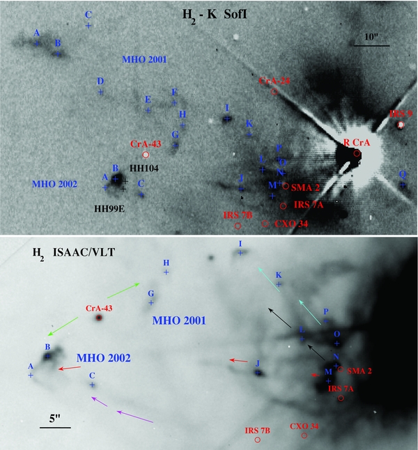
Figure 22. Upper panel: SofI H2 continuum-subtracted image of MHO 2001 and 2002 in the Coronet region. Labels and crosses indicate names and positions of detected knots and sub-structures along the flows. Lower panel: close-up view of the region at 2.12 μm, from a ISAAC/VLT image in logarithmic scale.
Download figure:
Standard image High-resolution imageB.2. P.M.s
A quick inspection of Figure 17 confirms that all the studied knots, except MHO 2008 D, are launched by YSOs inside or close to the Coronet. As already noted in Section 6.1, several flows originate in the eastern part of the Coronet, in particular in a region a few arcseconds around SMA 2, which encloses several early stage YSOs (see Appendix A and, e.g., Nutter et al. 2005; Groppi et al. 2007). This can be seen in more detail in Figure 23. MHO 2002 A is the terminal bow-shock of a west–east flow (MHO 2001 J, M), which has MHO 2001 Q as a flow counterpart. MHO 2002 C is likely part of another flow from IRS7 B. MHO 2002 B and MHO 2001 G are the southeastern and northwestern lobes of the CrA-43 (SMM 2) outflow. Then MHO 2001 D–N are part of one or more outflows roughly moving toward the northeast and emanate from the SMA 2 region.
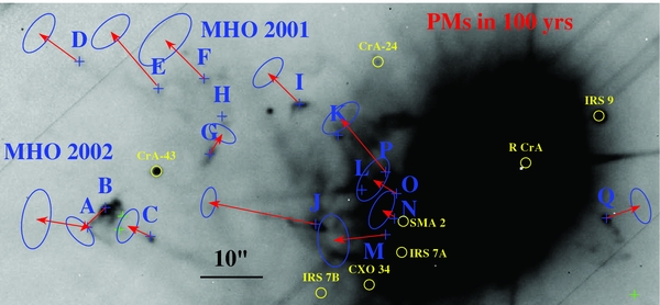
Figure 23. H2 flow chart of MHO 2001 and 2002. Proper motions in 100 yr and their error bars are indicated by arrows and ellipses, respectively.
Download figure:
Standard image High-resolution imageFigure 24 shows the flow charts of MHO 2009, 2011, 2012 and part of MHO 2001 A and B, which move from west to east and from west-southwest to east-northeast, being indeed the prosecution of the flows of Figure 23. Figure 25 shows P.M.s in MHO 2000 and 2013. Our multi-epoch images allow us to get a better measurement of the P.M. for MHO 2000 A, which appears to originate from a region around IRS 9 and CrA-24. On the other hand, MHO 2000 B is moving eastward and might not be related to this flow, but rather to MHO 2013, which appears as an expanding shell moving toward east-northeast, in this case IRS 6 is likely the driving source.
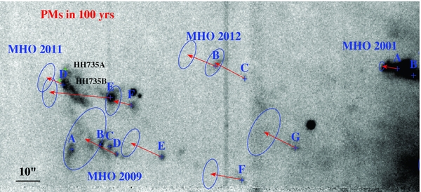
Figure 24. H2 flow chart of MHO 2009, 2011, 2012, and part of MHO 2001. Proper motions in 100 yr and their error bars are indicated by arrows and ellipses, respectively.
Download figure:
Standard image High-resolution image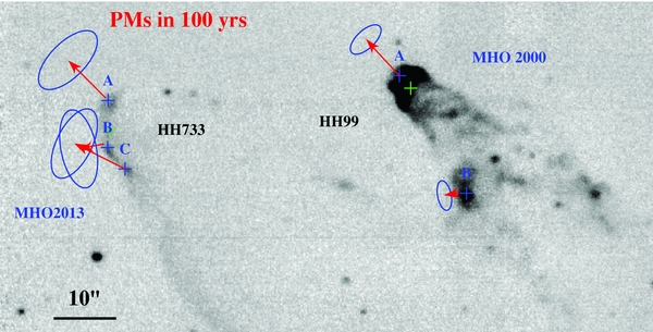
Figure 25. H2 flow chart of MHO 2000 and 2013. Proper motions in 100 yr and their error bars are indicated by arrows and ellipses, respectively.
Download figure:
Standard image High-resolution imageMHO 2014 (see Figure 26) is roughly moving toward north-northeast, and it is likely an expanding bow-shock, which originates from the western outskirts of the Coronet. Unfortunately, the lack of a second-epoch image for knots D and E does not allow us to completely reconstruct its motion.
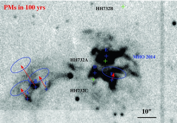
Figure 26. H2 flow chart of MHO 2014. Proper motions in 100 yr and their error bars are indicated by arrows and ellipses, respectively.
Download figure:
Standard image High-resolution imageAPPENDIX C: NOTES ON INDIVIDUAL MHOs—SOUTH AND WEST REGIONS
C.1. Morphology
Figure 27 shows a SofI H2 image of flows located to the southwest of the Coronet. There are four MHO flows, roughly northeast–southwest oriented, escaping from the Coronet (MHO 2003, 2004, 2006–2008). MHO 2003, 2004 (Wilking et al. 1997; Caratti o Garatti et al. 2006; Davis et al. 2010) and the newly detected MHO 2006, 2007 and 2008 are the molecular counterparts of HH 100, HH 104, HH 97, HH 101, and HH 731 (see, e.g., Strom et al. 1974; Hartigan & Graham 1987; Wang et al. 2004), respectively.
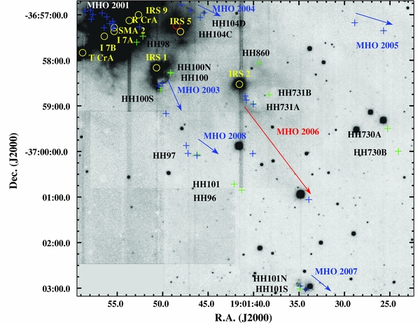
Figure 27. SofI H2 image of the southwestern flows detected outside the Coronet. MHO 2001 knots inside the Coronet are labeled with blue crosses.
Download figure:
Standard image High-resolution imageFigure 28 shows an ISAAC H2 continuum-subtracted image of MHO 2004 (i.e., HH 104 C and D). The molecular object, positioned about 20'' southwest of IRS 6, appears as a faint curved jet with three bright condensations (namely B–D), northeast–southwest oriented, and a brighter bow-shock (A or HH 104 C) placed ∼8'' northwest off-axis from the jet and east–west oriented. The bow-shock should not be associated with the main jet, which is likely driven by IRS 6.

Figure 28. ISAAC H2 continuum-subtracted image of MHO 2004 (see Figure 27). Labels and crosses indicate names and positions of detected knots and sub-structures along the flows.
Download figure:
Standard image High-resolution imageMHO 2003 (see Figure 27) is positioned about 20'' southwest of IRS 1 (or HH 100 IR), which is likely the driving source. A close-up view of the flow (see Figure 29) with ISAAC shows two bright asymmetric arcs (A and B) close to the source, and two fainter trails about 10'' and 40'' farther to the southwest. The H2 emission overlaps well with the CO 3–2 blueshifted outflow ejected by IRS 1 (van Kempen et al. 2009). The flow has a P.A.∼203°.

Figure 29. ISAAC H2 continuum-subtracted image of MHO 2003 (see Figure 27). Labels and crosses indicate names and positions of detected knots and sub-structures along the flows.
Download figure:
Standard image High-resolution imageMHO 2008 (A–C), located about 1' to the southwest and well aligned with the previous flow (see Figure 27), could be part of MHO 2003. On the other hand, MHO 2008 D is a bow-shock east–west oriented and should not be part of the flow (see Figure 30), but it is likely driven by the Class II source CrA 41.

Figure 30. ISAAC H2 continuum-subtracted image of MHO 2008 (see Figure 27). Labels and crosses indicate names and positions of detected knots and sub-structures along the flows.
Download figure:
Standard image High-resolution imageMHO 2006 (A–C) is a trail of faint precessing knots (P.A. ∼ 206°), located about 15'' to the southwest of IRS 2 (see Figure 31), which is the driving source. MHO 2006 D (see Figure 27) is a faint patch and could be part of the flow.
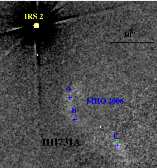
Figure 31. ISAAC H2 continuum-subtracted image of MHO 2006 (see Figure 27). Labels and crosses indicate names and positions of detected knots and sub-structures along the flows.
Download figure:
Standard image High-resolution imageAbout 6' southwestward of the Coronet, we detect MHO 2007, the molecular counterpart of HH 101 (see Figure 27). The MHO extends for roughly 40'', north-northeast–south-southwest elongated, with two faint arcs in front, likely a bow-shock structure and several bright scattered knots behind (A and B are particularly bright). The MHO is shown in Figure 32, where an ISAAC H2 continuum-subtracted image is shown.

Figure 32. ISAAC H2 continuum-subtracted image of MHO 2007, the molecular counterpart of HH 101 (see Figure 27). Labels and crosses indicate names and positions of detected knots and sub-structures along the flows.
Download figure:
Standard image High-resolution imageThe last newly detected flow, MHO 2005 (knots A–I), is located ∼4' to the west of the Coronet and extends for about 6' around S CrA (see Figures 33 and 34), roughly showing a broad S-shape. Knots C and E, the brightest knots of the flow, along with D, are the molecular counterpart of HH 82 B and A, respectively. Knot F is positioned about 1' south and might not be part of the flow. The HH 729 knots, which should be driven by S CrA (see, e.g., Strom et al. 1974; Wang et al. 2004), are not detected in our H2 images.
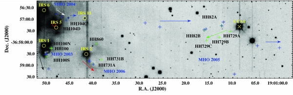
Figure 33. SofI H2 image of the western flows detected outside the Coronet.
Download figure:
Standard image High-resolution image
Figure 34. SofI H2 continuum-subtracted image of MHO 2005 (see Figure 33).
Download figure:
Standard image High-resolution imageC.2. P.M.s
Figure 35 shows the MHO 2004 A P.M., confirming that the bow-shock is not related to the main jet, but is moving west-northwest, possibly associated with the same flow as MHO 2001 Q.

Figure 35. H2 flow chart of MHO 2004. Proper motions in 100 yr and their error bars are indicated by arrows and ellipses, respectively.
Download figure:
Standard image High-resolution imageFinally, our kinematical analysis reveals three or four different flows in the CrA southwestern region, as shown in Figures 36, 37, and 38. MHO 2003 and knots A–C of MHO 2008 are likely part of the same flow (Figure 36) moving toward the southwest. On the other hand, knot D stands alone moving toward the south-southwest (Figure 37), likely driven by the nearby YSO candidate CrA-41, and MH0 2006 (same figure) represents another flow. MHO 2007 (Figure 38) is roughly aligned with the MHO 2003–6 flow, with similar tangential velocities. However, it is not clear whether or not it could be part of it, because of the different orientation of the leading bow-shock, which rather points to the south-southwest.
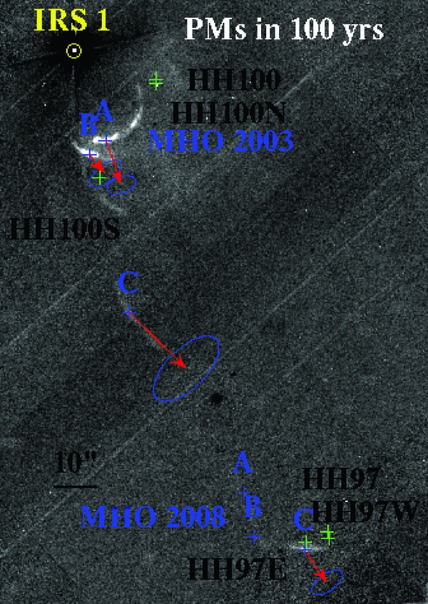
Figure 36. H2 flow chart of MHO 2003 and part of MHO 2008. Proper motions in 100 yr and their error bars are indicated by arrows and ellipses, respectively.
Download figure:
Standard image High-resolution image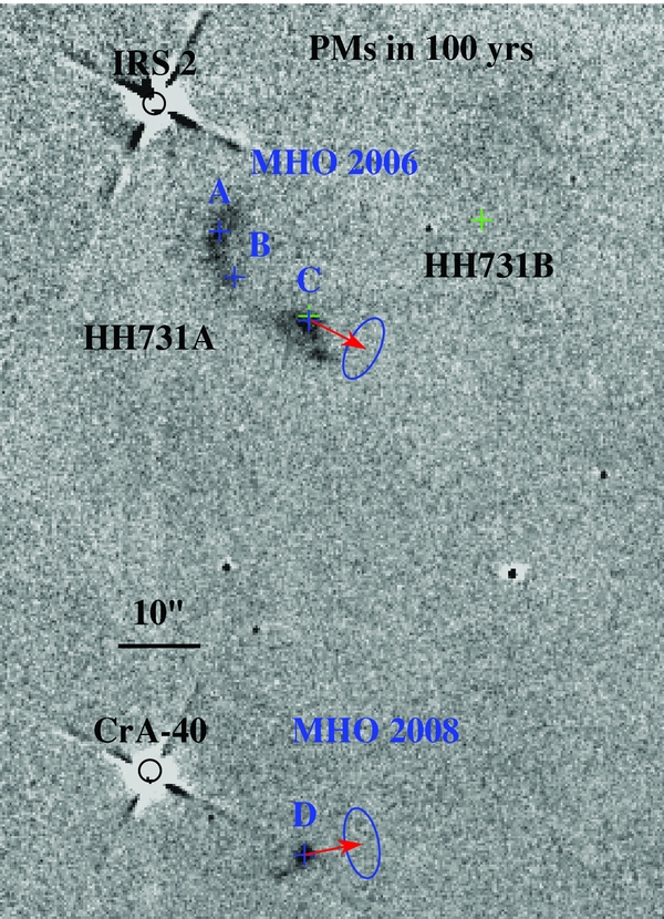
Figure 37. H2 flow chart of MHO 2006 and part of MHO 2008. Proper motions in 100 yr and their error bars are indicated by arrows and ellipses, respectively.
Download figure:
Standard image High-resolution image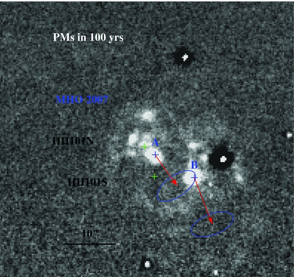
Figure 38. H2 flow chart of MHO 2007. Proper motions in 100 yr and their error bars are indicated by arrows and ellipses, respectively.
Download figure:
Standard image High-resolution imageAPPENDIX D: NOTES ON INDIVIDUAL SPITZER FLOWS
The first outflow detected in our Spitzer maps, named Spitzer outflow 1, is located on the western edge of the CrA star-forming region, about 17' from the Coronet. Figure 39 (upper right-hand panel) shows the morphology of the outflow, which is composed of several knots and bow-shocks, roughly east–west oriented. These knots likely originate from a precessing jet, as indicated by their scattered placement. No obvious counterpart on the eastern edge of CrA is observed.
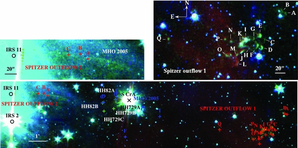
Figure 39. Spitzer three-color image of Spitzer outflow 2 (upper left), Spitzer outflow 1 (upper right), and the entire region including Spitzer outflow 1, Spitzer outflow 2, and MHO 2005 (bottom), made from the IRAC 3.6 μm (blue), 4.5 μm (green), and 8 μm (red) images. Labels indicate the position of the newly detected knots (EGOs) and MHO 2005 A and B.
Download figure:
Standard image High-resolution imageSpitzer outflow 2, located ∼1' west of IRS 11 (see Figure 39, upper left-hand panel), is a curved jet which includes MHO 2005 A and B, but is not detected in our H2 SofI map, because it is slightly below the detection limit. It is worth noting that Spitzer outflow 1 and 2, along with MHO 2005, could be part of a larger east–west precessing flow (see Figure 39, bottom panel), possibly driven by a YSO inside the Coronet. On the other hand, as seen in Figure 39 (bottom panel), the bulk of Spitzer outflow 1 is well aligned with IRS 2, and thus it is not clear which is the driving source.
The IRAS 32 outflow, the third Spitzer flow discovered (P.A.∼39°), originates from IRAS 32, and has a clear precessing morphology, as seen in Figure 40. The outflow extends for ∼203, i.e., it has a projected length of about 0.77 pc. Knots from A to E are part of the northeastern lobe, while knots from F to N, along with HH 861 A, B, and HH 862 are located in the southwestern lobe. The shock-excited nature of these knots is revealed by our H2 image taken with ISAAC/VLT (lower left panel of Figure 40), centered around the YSO. Due to the small FoV, we could only identify the closest knots (i.e., D–G), which thus we also labeled as MHO 2010. Our H2 and Ks images also show the two outflow cavities, illuminated by scattered light from the YSO. In between the two cavities, a dark band is well visible, possibly indicating the presence of a disk.

Figure 40. Spitzer three-color image of the IRAS 32 (IRAS 18595-3712) outflow, made from the IRAC 3.6 μm (blue), 4.5 μm (green), and 8 μm (red) images. Labels indicate the position of the newly detected knots (EGOs), MHO 2010, and previously known HH objects. The lower left panel displays a close-up view of the inner region of the outflow at 2.12 μm, showing the inner knots, the outflow cavities, and a possible disk.
Download figure:
Standard image High-resolution image
Footnotes
- 12
The distance to CrA is based on measurements to several stars, ranging from 85 to 190 pc. A comprehensive summary of the various measurements can be found in Neuhäuser & Forbrich (2008); throughout this paper, we use their suggested distance of 130 pc.
- 13
The Submillimeter Array is a joint project between the Smithsonian Astrophysical Observatory and the Academia Sinica Institute of Astronomy and Astrophysics and is funded by the Smithsonian Institution and the Academia Sinica.
- 14
- 15
- 16