


ABSTRACT
We describe the Hubble Space Telescope (HST) Wide Field Camera 3 (WFC3) Early Release Science (ERS) observations in the Great Observatories Origins Deep Survey (GOODS) South field. The new WFC3 ERS data provide calibrated, drizzled mosaics in the UV filters F225W, F275W, and F336W, as well as in the near-IR filters F098M (Ys), F125W (J), and F160W (H) with 1–2 HST orbits per filter. Together with the existing HST Advanced Camera for Surveys (ACS) GOODS-South mosaics in the BViz filters, these panchromatic 10-band ERS data cover 40–50 arcmin2 at 0.2–1.7 μm in wavelength at 0 07–015 FWHM resolution and 0090 Multidrizzled pixels to depths of AB ≃ 26.0–27.0 mag (5σ) for point sources, and AB ≃ 25.5–26.5 mag for compact galaxies. In this paper, we describe (1) the scientific rationale, and the data taking plus reduction procedures of the panchromatic 10-band ERS mosaics, (2) the procedure of generating object catalogs across the 10 different ERS filters, and the specific star–galaxy separation techniques used, and (3) the reliability and completeness of the object catalogs from the WFC3 ERS mosaics. The excellent 007–015 FWHM resolution of HST/WFC3 and ACS makes star–galaxy separation straightforward over a factor of 10 in wavelength to AB ≃ 25–26 mag from the UV to the near-IR, respectively. Our main results are: (1) proper motion of faint ERS stars is detected over 6 years at 3.06 ± 0.66 mas year−1 (4.6σ), consistent with Galactic structure models; (2) both the Galactic star counts and the galaxy counts show mild but significant trends of decreasing count slopes from the mid-UV to the near-IR over a factor of 10 in wavelength; (3) combining the 10-band ERS counts with the panchromatic Galaxy and Mass Assembly survey counts at the bright end (10 mag ≲ AB ≲ 20 mag) and the Hubble Ultra Deep Field counts in the BVizYsJH filters at the faint end (24 mag ≲ AB ≲ 30 mag) yields galaxy counts that are well measured over the entire flux range 10 mag ≲ AB ≲ 30 mag for 0.2–2 μm in wavelength; (4) simple luminosity+density evolution models can fit the galaxy counts over this entire flux range. However, no single model can explain the counts over this entire flux range in all 10 filters simultaneously. More sophisticated models of galaxy assembly are needed to reproduce the overall constraints provided by the current panchromatic galaxy counts for 10 mag ≲ AB ≲ 30 mag over a factor of 10 in wavelength.
Export citation and abstract BibTeX RIS
1. INTRODUCTION
The study of the formation and evolution of galaxies and large-scale structure are amongst the most active interfaces between theory and observation in modern astrophysics. Galaxies are believed to have formed gradually over cosmic time from a combination of gas infall and mergers (Hopkins et al. 2006), regulated by feedback from stellar winds, supernovae (SNe), and/or active galactic nuclei (AGNs; e.g., Scannapieco et al. 2005; di Matteo et al. 2005). The origin of the Hubble sequence is not yet fully understood (e.g., Driver et al. 1998) but is likely related to the balance between major mergers versus minor accretion events and steady infall (e.g., Conselice et al. 2003; Hopkins et al. 2010; Peng et al. 2010). The critical epoch for the assembly of massive galaxies appears to be the ∼4 Gyr span from redshift z≃ 3 to z≃ 1, where also the cosmic star formation history seems to have peaked (Madau et al. 1998; Hopkins 2004; Hopkins & Beacom 2006).
At redshifts ≳2–3, deep Hubble Space Telescope (HST) imaging surveys and ground-based spectroscopy have revealed a paucity of massive galaxies and few classical disks or spheroids (e.g., Law et al. 2007, 2009). In contrast, large ground-based spectroscopic surveys targeting redshifts z ≲ 1—coupled with HST imaging—have shown that by this epoch massive galaxies are largely mature, and that the Hubble sequence has been mostly established (e.g., Abraham et al. 1996, 1999, 2007; Driver et al. 1995, 1998; Glazebrook et al. 1995; Lilly et al. 1998). While substantial growth (∼50%) in the stellar mass of all galaxy types—including spheroids—may have occurred during the last ∼7 Gyr, the process of major galaxy assembly was well underway by z≃ 1 (e.g., de Lucia et al. 2006; Dickinson et al. 2003). The interim period—from redshifts of z≃ 3 to z≃ 1—is the era in which much of the stellar mass in galaxies is accumulated (e.g., Dickinson et al. 2003; Abraham et al. 2007), and when galaxies acquire the characteristic structural and dynamical properties that define them today. The HST Wide Field Camera 3 (WFC3) was optimized to study this critical period of galaxy assembly.
WFC3 was successfully installed into HST on 2009 May 14, by the astronauts on board Space Shuttle Atlantis during the Space Transportation System mission 125 (STS-125). This shuttle mission was the fifth Servicing Mission of HST, however, for historical reasons, it is referred to as SM4. Many of the current co-authors were members of the WFC3 Science Oversight Committee (SOC) from 1998 July through 2009 November. Our main role as the SOC was to define the WFC3 science requirements and goals, monitor them during the pre-launch phases of the project, and to oversee the design, implementation, integration, and testing (both ground-based and on-orbit) of the WFC3 instrument.
The WFC3 provides a unique opportunity to compare the galaxy populations in the local and distant universe. With its wide spectral coverage (0.2–1.7 μm), very high spatial resolution (004 FWHM at 0.2 μm to 016 FWHM at 1.6 μm), fine pixel sampling (0039 pixel−1 in the UVIS channel and 013 pixel−1 in the IR channel), and high sensitivity (AB ≃ 26–27 mag in two orbits; 5σ for point sources), many new interesting questions and outstanding problems can be addressed with the WFC3 data. By sampling the vacuum UV with high sensitivity and the very high angular resolution afforded by the diffraction limited 2.4 m Hubble Space Telescope, WFC3 can observe star-forming regions in galaxies over most of the Hubble time. The near-IR channel on WFC3 allows one to do rest-frame visible-band photometry of distant galaxies to low luminosities and over areas large enough to provide representative samples. Together, the panchromatic images produced by WFC3 allow the user to decompose distant galaxies into their constituent substructures, examine their internal stellar populations, and help constrain their dust content. In this Early Release Science (ERS) program, the UVIS and IR channels of WFC3 are used to provide a small, but representative sampling of the capabilities of WFC3 to examine the formation and evolution of galaxies in the critical galaxy assembly epoch of z≃ 1–3, when the universe was only 6–2 Gyr old, respectively.
Details of the HST WFC3 ERS program (PID 11359; PI: R. O'Connell) can be found on the Web.25 The current ERS program was specifically conceived to make maximum use of these WFC3 capabilities, and to make an optimal comparison between the intermediate- and high-redshift galaxy samples identified in the current ERS program and nearby galaxies imaged in other HST programs. These capabilities were important WFC3 science drivers, while the instrument was designed and constructed from 1998 to 2008.
In the year that the intermediate-redshift WFC3 ERS data have been available, a number of papers have appeared or submitted that use this panchromatic data set. For instance, Ryan et al. (2011) discuss the evolution of passive galaxies using the WFC3 ERS observations and make a detailed study of their size evolution over cosmic time. Rutkowski et al. (2011) present a panchromatic catalog of early-type galaxies at intermediate redshifts (z ≃ 0.3–1.5) from the WFC3 ERS data and derive their rest-frame (FUV–V) and (NUV–V) colors as a function of redshift. Cohen et al. (2011) present a 10-band photometric study of distant galaxies in the WFC3 ERS data, measure reliable photometric redshifts, and derive their physical properties with cosmic time. Hathi et al. (2010) discuss UV-dropout galaxies in the Great Observatories Origins Deep Survey (GOODS)-South at redshifts z≃ 1.5–3 from the WFC3 ERS data, and summarize the evolution of the faint-end luminosity function (LF) slope α and characteristic luminosity L* from z≃ 8 to z≃ 0. Oesch et al. (2010b) similarly discuss the evolution of the ultraviolet LF from z ∼ 0.75 to z ∼ 2.5. Straughn et al. (2011) study faint emission-line galaxies from the WFC3 ERS IR grism observations. Van Dokkum & Brammer (2010) discuss WFC3 grism spectra and images of one growing compact galaxy at z≃ 1.9. Finkelstein et al. (2011) discuss spatially resolved imaging of Lyα emission line objects at z≃ 4.4 through parallel ACS F658N narrow-band images to the WFC3 ERS data, and their constraints as to how Lyman continuum photons escape from such objects.
Labbé et al. (2010) discuss the star formation rates and stellar masses of z≃ 7–8 galaxies from IRAC observations of the WFC3/IR ERS and Hubble Ultra Deep Fields (HUDFs). Robertson (2010) estimates how to best improve the LF constraints from high-redshift galaxy surveys using WFC3 ERS data and from additional deep WFC3 survey data yet to be obtained. Bouwens et al. (2010a) discuss potentially very blue UV-continuum slopes of low luminosity galaxies at z≃ 7 from the WFC3 ERS IR data, and their possible implications for very low metallicities in these objects. Bouwens et al. (2010b) also discuss z≃ 8 galaxy candidates seen in the ultradeep WFC3/IR observations of the HUDF. Yan et al. (2011a) probe the bright end of the galaxy LF at z ≳ 7 using HST pure parallel observations, and discuss these in context of the WFC IR observations in the ERS and in the HUDF. Yan et al. (2011b) discuss galaxy formation in the reionization epoch from the WFC3 observations of the HUDF, and suggest an LF at z≃ 8–10 that differs from that found by Bouwens et al. (2010b) and Oesch et al. (2010a). Wyithe et al. (2011) explain that part of this discrepancy may arise due to distortion of the very high redshift galaxy number counts through gravitational lensing by random foreground galaxies at z≃ 1–2. This boosts the number of z ≳ 8–10 objects that become observable in the WFC3 IR samples, a non-negligible fraction of which therefore must be sought close to foreground galaxies at z≃ 1–2. These many examples show the great potential of the WFC3 ERS data presented in the current paper, and we refer the reader to these other papers for in-depth studies of the ERS data that are beyond the scope of the current paper. It suffices to say that the quality of and the scientific results from the ERS data exceeded the expectations of the WFC3 SOC, even though we have been involved with the WFC3 instrument from its conception in 1998.
In Section 2 of this paper, we present the WFC3 ERS survey strategy, the filters used and their achieved depths. In Section 3, we present the observations in both the WFC3 UVIS and IR channels, and the pointings and their areal coverage. In Section 4, we present the WFC3 data reduction procedures, their reliability and completeness, and their current limitations. In Section 5, we present the object finding procedures and catalog generation, and the star–galaxy separation procedure used and its reliability in the 10 ERS filters. In Section 6, we present the panchromatic ERS star counts and discuss the faint ERS stellar proper motion results. In Section 7, we present the panchromatic ERS galaxy counts from 0.2–1.7 μm to AB ≃ 26–27 mag, and compare these to the 10-band ground-based Galaxy and Mass Assembly (GAMA) survey counts for 10 mag ≲ AB ≲ 20 mag at the bright end, and to the HUDF counts in the BVizYsJH filters (defined in Section 2.1) for 24 mag ≲ AB ≲ 30 mag at the faint end. We also present the panchromatic ERS images for interesting individual objects. In Section 8, we summarize our main results and conclusions. Throughout this paper, we use Wilkinson Microwave Anisotropy Probe (WMAP) year 7 cosmology (Komatsu et al. 2011), or H0 = 71 km s-1 Mpc−1, Ω0 = 0.26, and Λ = 0.74, and the ABν magnitude system (Oke 1974).
2. WFC3 AND ITS CAPABILITIES
2.1. The ERS Filter Set
In the current ERS program, the unique panchromatic capabilities of WFC3 are used to survey the structure and evolution of galaxies at the peak of the galaxy assembly epoch at z≃ 1–3. Deep ultraviolet and near-IR imaging, and slitless near-IR spectroscopy of existing deep multi-color GOODS-S/ACS fields are used to gauge star formation and the growth of stellar mass as a function of galaxy morphology, structure and surrounding density in this critical cosmic epoch at redshifts 1 ≲ z ≲ 3.
The total HST filter set provided by the WFC3 ERS imaging of the GOODS-South field is shown in Figure 1(a), and its properties are summarized in Tables 1 and 2. WFC3 adds the F225W, F275W, and F336W filters in the WFC3 UVIS channel, and the F098M, F125W, and F160W filters (hereafter YsJH) in the WFC3 IR channel. Together with the existing GOODS ACS F435W, F606W, F775W, and F850LP images (Giavalisco et al. 2004), the new WFC3 UVIS and IR filters provide a total of 10 HST filters that span the wavelength range λ ≃ 0.2–1.7 μm nearly contiguously. We refer to this entire 10-band survey hereafter as the "ERS," to these 10 filters as the "ERS filters," and to the seven reddest ERS filters as the "BVizYsJH" filters throughout. Details of the GOODS survey can be found in Giavalisco et al. (2004) and references therein. The top panel of Figure 1(a) compares the ERS filters to the spectral energy distribution (SED) of two single burst model galaxies (middle and bottom panels of Figure 1(a)) with ages of 0.1 and 1 Gyr at redshifts of z = 0, 2, 4, 6, and 8, respectively.
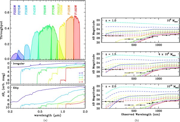
Figure 1. (a) Top panel: the full panchromatic HST/WFC3 and ACS filter set used in the ERS imaging of the GOODS-South field. Plotted is the overall system throughput, or the HST Optical Telescope Assembly throughput OTA × filter transmission T × detector QE. Middle and bottom panels: spectral energy distributions for two single burst model galaxies with ages of 0.1 and 1 Gyr and redshifts of z = 0, 2, 4, 6, and 8 are shown as black, blue, green, yellow, and red curves, respectively. Intergalactic medium absorption shortward of Lyα was applied following Haardt & Madau (1996). The UVIS filters sample the Lyα forest and Lyman continuum breaks, while the near-IR filters probe the 4000 Å and Balmer breaks at these redshifts. Additional photometry is available from ground-based VLT K-band imaging, and Spitzer/IRAC imaging at 3.5, 4.5, 5.6 and 8.5 μm. (b) Mass sensitivity of the WFC3 ERS filters used. The three panels show the depth of the WFC3 ERS images as horizontal bars, compared to evolving galaxy models of different masses at three redshifts. The top panel is for z = 1 and a stellar mass of 109 M☉. The solid lines represent nearly instantaneous bursts, and the dashed lines are for declining star formation with a 1 Gyr e-folding time. The colors refer to ages of 10, 100, 500, 1000, 1400, 2000, and 3000 Myr from cyan to red. The middle panel shows similar models at z = 1.5 for 4 × 10⁹ M☉, while the bottom panel is for z = 2 and masses of 1010 M☉. At z = 1, the WFC3 ERS reaches masses of 0.02 M* for typical star formation histories. Both the flux scale and the wavelength scale are logarithmic, illustrating WFC3's exquisite panchromatic coverage and sensitivity in probing the stellar masses of galaxies through its IR channel, and the star formation in galaxies through its UVIS channel.
Download figure:
Standard image High-resolution imageTable 1. Filters, Exposure Times, and Depths of the WFC3 ERS and GOODS-South ACS Data
| Channel | Filter1 | Filter2 | Filter3 | Filter4 | Grism | Grism | Total Orbits |
|---|---|---|---|---|---|---|---|
| WFC3/UVIS | F225W | F275W | F336W | ⋅⋅⋅ | |||
| Orbits | 2 | 2 | 1 | ⋅⋅⋅ | 5 × 8 = 40 Direct | ||
| Depth (AB) | 26.3 | 26.4 | 26.1 | ⋅⋅⋅ | |||
| nJy | 110 | 100 | 132 | ⋅⋅⋅ | |||
| ACS/WFC | F435W | F606W | F775W | F850LP | G800L | ||
| Orbits | 3 | 3 | 4 | 9 | 80 | 15 × 19 = 285 Direct | |
| Depth (AB) | 27.9 | 28.1 | 27.5 | 27.3 | 27.0 | 2 × 20 = 40 Grism | |
| nJy | 14 | 14 | 27 | 44 | 58 | ||
| WFC3/IR | F098M | F125W | F160W | G102 | G141 | ||
| Orbits | 2 | 2 | 2 | 2 | 2 | 6 × 10 = 60 Direct | |
| Depth (AB) | 27.2 | 27.55 | 27.25 | 25.2 | 25.5 | 1 × 4 = 4 Grism | |
| nJy | 48 | 36 | 48 | 303 | 230 | ||
| Total WFC3 ERS Orbits | (2009 Aug–2009 Oct) | 104 | |||||
| Total ACS GOODS Orbits inside ERS | (2002 Jul–2005 Mar) | 325 | |||||
| Total HST Orbits | (2002 Jul–2009 Oct) | 429 | |||||
Notes. Note 1: the orbital integration times listed are those as achieved for the WFC3 UVIS and IR ERS observations, as well as for the GOODS ACS v2.0 observations. For the ACS grism, 40 out of 200 orbits ACS G800L observations from the HST Cycle 14 PEARS project 10530 (PI: S. Malhotra; Malhotra et al. 2005; Pirzkal et al. 2004, 2005, 2009; Straughn et al. 2008, 2009) that reside inside the ERS mosaic are listed (see Figure 3). Note 2: the listed depth is the 50% completeness limit for 5σ detections in total SExtractor AB magnitudes for typical compact objects at this flux level (circular aperture with 04 radius; 0.50 arcsec2 aperture), as derived from Figure 9. Note 3: for spectral continuum detection in the G102 and G141 grisms, these flux limits are about 2.0–1.8 mag brighter, respectively. Note 4: we note that the pre-flight WFC3 ETC sensitivity values were 0.15–0.2 mag more conservative in both the UVIS and the IR than the in-flight values quoted here in Table 1, as also shown in Figure 2. Note 5: due to the limited observing time available, and its poorer prism performance, UV-prism observations in P280 were not taken as part of the ERS.
Download table as: ASCIITypeset image
Table 2. ERS Filters, PSFs, Zero Points, Sky Background, and Effective Area
| HST- | ERS | Central | Filter | PSF | Zero Point | Sky | Effective |
|---|---|---|---|---|---|---|---|
| Instrument/ | Filter | Lambda | FWHM | FWHM | (AB mag@ | Background | Area |
| Mode | (μm) | (μm) | ('') | 1 e− s−1) | magarcsec−2 | (arcmin2) | |
| WFC3/UVIS | F225W | 0.2341 | 0.0547 | 0.092 | 24.06 | 25.46 | 53.2 |
| WFC3/UVIS | F275W | 0.2715 | 0.0481 | 0.087 | 24.14 | 25.64 | 55.3 |
| WFC3/UVIS | F336W | 0.3361 | 0.0554 | 0.080 | 24.64 | 24.82 | 51.6 |
| ACS/WFC | F435W | 0.4297 | 0.1038 | 0.080 | 25.673 | 23.66 | 72.4 |
| ACS/WFC | F606W | 0.5907 | 0.2342 | 0.074 | 26.486 | 22.86 | 79.2 |
| ACS/WFC | F775W | 0.7764 | 0.1528 | 0.077 | 25.654 | 22.64 | 79.3 |
| ACS/WFC | F850LP | 0.9445 | 0.1229 | 0.088 | 24.862 | 22.58 | 80.3 |
| WFC3/IR | F098M | 0.9829 | 0.1695 | 0.129 | 25.68 | 22.61 | 44.8 |
| WFC3/IR | F125W | 1.2459 | 0.3015 | 0.136 | 26.25 | 22.53 | 44.7 |
| WFC3/IR | F160W | 1.5405 | 0.2879 | 0.150 | 25.96 | 22.30 | 44.7 |
Notes. Note 1: the panchromatic PSF FWHM was measured from ERS stars as in Figures 7(a) and (b), and includes the contribution from the OTA and its wavefront errors, the specific instrument pixel sampling or Modulation Transfer Function (MTF). Note 2: the WFC3 zero points are in AB magnitudes for 1.0 e− s−1, taken from http://www.stsci.edu/hst/wfc3/phot_zp_lbn. Note 3: the GOODS BViz sky-background values are from Hathi et al. (2008). Note 4: the effective areas used in this paper are in units of arcminutes squared for the effective number of WFC3 or ACS tiles available and used. Note 5: the GOODS v2.0 BViz data release is from http://archive.stsci.edu/pub/hlsp/goods/v2/h_goods_v2.0_rdm.html. Note 6: the panchromatic effective ERS area was derived from Figures 8(a)–(c) for the WFC3 mosaics and the relevant GOODS tiles, and indicates the total area over which at least half of the total ERS exposure time was available. (Figure 8 shows that ≳80% of the total ERS exposure time was available for 50 arcmin2 in the WFC3 UVIS filters, and for 40 arcmin2 in the WFC3 IR filters.)
Download table as: ASCIITypeset image
The ERS images in the WFC3 UVIS filters F225W, F275W, and F336W are used to identify galaxies at redshifts z ≳ 1.5 from their UV continuum breaks, which between the F225W and F275W filters is sampled at redshifts as low as z≃ 1.5–1.7 (see Figure 1). These filters provide star formation indicators tied directly to both local and z ≳ 3 galaxy populations, which are the ones best observed through their Lyman breaks from the ground at λ ≳ 350 nm. The critical new data that the WFC3 UVIS channel can provide are thus very high resolution, deep images for 0.2 μm ≲ λ ≲ 0.36 μm, as illustrated in Figure 1(a).
The ERS images in the WFC3 near-IR filters F098M, F125W, and F160W are used to probe the Balmer and 4000 Å breaks and stellar mass function well below 109 M☉ for mass-complete samples in the critical redshift range of z≃ 1–3. The unique new data that the WFC3 IR channel can provide are high-resolution, very sensitive near-IR photometry over fields larger than those possible with HST NICMOS, or over wide fields with adaptive optics from the ground (e.g., Steinbring et al. 2004; Melbourne et al. 2005).
2.2. ERS Grisms
In addition to these broadband ERS filters, we used the WFC3 near-IR grisms G102 and G141 to obtain slitless spectroscopy of hundreds of faint galaxies at a spectral resolution of R≃ 210–130, respectively. The WFC3 near-IR grism data can trace the primary indicators of star formation—the Lyα and H-α emission-lines—in principle over the redshift range for z≃ 5–13 and z≃ 0.2–1.7, respectively. WFC3 can also trace the Lyman break and the rest-frame UV continuum slope, as well as the Balmer and 4000 Å breaks over the redshift range z≃ 1–9 and z≃ 0–2.5, respectively. The ERS grism program thus at least covers the peak of the cosmic star formation history at redshifts 1 ≲ z ≲ 2, using some of the most important star formation and post-starburst indicators, while also providing some metallicity-independent reddening indicators. Both IR grism dispersers provide capabilities that cannot be reproduced from the ground: slitless spectroscopy of very faint objects (AB ≃ 25–26 mag) over a contiguous wide spectral range in the near-IR, that is not affected by atmospheric night-sky lines. The ERS grism observations are two orbits in depth each, covering a single WFC3 field, which was also covered in a previous ACS G800L grism survey (Straughn et al. 2009). An example of the ERS G141 and G102 grism spectra is shown in the figures of Appendix B.2. Further details of the ERS grism data reduction and the analysis of the faint emission line galaxies are given in Appendix B.2 and by Straughn et al. (2011).
WFC3 UVIS G280 UV-prism observations were not made as part of the 104 orbit intermediate-redshift ERS program, because of its much lower throughput and the significant overlap of its many spectral orders (Bond & Kim Quijano 2007; Wong et al. 2010). Currently, one Cycle 17 GO program (11594; PI: J. O'Meara) is using the WFC3 G280 prism to carry out a spectroscopic survey of Lyman limit absorbers at redshifts 1.8 ≲ z ≲ 2.5. Readers interested in the WFC3 G280 prism performance should follow the results from that program.
2.3. ERS UVIS Filter Red-leaks and IR Filter Blue-leaks
In the context of the WFC UVIS and IR channel performance for intermediate- to high-redshift early- and late-type galaxies, it is useful to briefly summarize here the possible effects of UVIS channel filter red-leaks and IR channel filter blue-leaks on the measured fluxes of these objects. UVIS red-leaks are defined as the fraction of flux longward of 400 nm of an SED of given effective temperature Teff that makes it erroneously into the UV filter. The IR blue-leaks are defined as the fraction of flux shortward of 830 nm of an SED of given effective temperature Teff that makes it erroneously into the IR filter or grism (for details, see Wong et al. 2010).
The WFC3 UVIS filters were designed with great attention to minimize their red-leaks, which were much larger in the earlier generation WFPC2 UV filters. Similarly, the WFC3 IR filters and grisms were designed to minimize the blue-leaks. For both sets of WFC3 filters, lower out-of-band transmission usually goes at the expense of lower in-band transmission, and vice versa. Hence, both the WFC3 and IR filters were designed and fabricated such that the in-band transmission was optimized as much as possible, while keeping the out-of-band transmission to acceptable or correctable levels for all SEDs expected in the relevant astrophysical situations.
The resulting WFC3 UVIS red-leaks are acceptably small (≲10%) for all zero-redshift SEDs with Teff ≳ 5000 K for the F225W filter, Teff≳ 4000 K for the F275W filter, and Teff ≳ 2000 K for the F336W filter, respectively (Wong et al. 2010). For cooler (Teff ≲ 2000–5000 K) zero-redshift SEDs, some red-leak correction thus has to be applied to the observed F336W, F275, and F225W fluxes, respectively. However, for objects at substantial redshifts (z ≳ 0.75–1), the SED will shift out of the UVIS sensitivity regime quickly enough to significantly reduce the red-leak. Hence, the WFC3 UVIS red-leaks in general only need to be corrected for the reddest (Teff ≲ 5000 K), lower-redshift (z ≲ 0.75) SEDs observed in the bluest UVIS filters (F225W). Further details are given in Rutkowski et al. (2011).
The WFC3 IR blue-leaks are very small (≲0.01%) for all zero-redshift SEDs with Teff ≲ 10,000 K for the F098M, F105W, F125W, and F160W filters, and remains very small (≲0.1%) even for the bluest zero-redshift SEDs with Teff ≃ 30,000–50,000 K (Wong et al. 2010). For higher-redshift SEDs (z ≳ 1) of any Teff, the redshift further reduces the IR blue-leak. Similarly, the G141 grism was made on a glass substrate with no transmission below 750 nm, and is well blocked by its coatings shortward of 1050 nm and long-ward of 1700 nm (Baggett et al. 2007). Hence, it also has acceptably an small blue-leak. The same is true for the higher-resolution G102 grism.
2.4. WFC3 Detectors and Achieved ERS Sensitivities
The WFC3 UV-blue optimized CCDs were chosen specifically to complement those of ACS. They were made by E2V in the UK, and are thinned, backside illuminated, CCD detectors with 2k × 4k 15 μm (00395) pixels, covering the wavelength range 200–1000 nm with Quantum Efficiency QE ≳ 50% throughout (Wong et al. 2010; Kimble et al. 2010). The total WFC3 UVIS field of view with these two CCDs is 162'' × 162''.
The WFC3 near-IR detectors were Teledyne HgCdTe infrared detectors (molecular beam epitaxy-grown and substrate removed) with Si CMOS Hawaii-1R multiplexers and have 1k × 1k 18 μm (0130) pixels, covering the wavelength range 800–1730 nm with QE ≳ 77% throughout (Wong et al. 2010; Kimble et al. 2010). The total WFC3 IR field of view is 123'' × 136''. Further specifications of the WFC3 detectors are listed where relevant below.
Table 1 summarizes the resulting WFC3 sensitivities from our relatively short ERS exposures. The table lists the number of orbits per filter and the 5σ depths in AB magnitudes and Fν units. A net exposure time of 2600–2700 s was available in each HST orbit for on-source ERS observations. In Figure 1(b), the equivalent depths are plotted in physical terms, by comparing with the spectral synthesis models of Bruzual & Charlot (2003) at the three fiducial redshifts, following Ryan et al. (2007, 2008, 2011). Simple stellar populations models with single bursts or exponentially declining star formation rates with an e-folding time of 1 Gyr are plotted. Figure 1(b) shows the predicted SEDs for models with ages ranging from 10 Myr to 3 Gyr, along with the 5σ depths of the WFC3 ERS program. The three panels represent redshifts z = 1.0, 1.5, and 2.0, and models with stellar masses of M = 109, 4 × 10⁹, and 1010 M☉, respectively. These SED tracks illustrate the intended SED and mass sensitivity of the WFC3 ERS observations as a function of cosmic epoch. Galaxies with ongoing star formation, even with fairly large ages, are easily detected in the WFC3 UV observations. At z ≃ 2, a maximally old τ ≃ 1 model with a mass of ∼0.3 M* is detectable above the WFC3 detection threshold in the F336W filter, while at z≃ 1, the WFC3 ERS can detect young star-forming galaxies with masses as low as a few × 107 M☉, or about a M ∼0.01 M* galaxy in that filter.
Table 2 summarizes the HST instrument modes and the ERS filters used, the filter central wavelength λ, its width, and the point-spread function (PSF) FWHM as a function of wavelength, the AB magnitude zero points for all 10 filters for a count rate of 1.0 e− s−1, as well as the zodiacal sky background measured in each ERS filter. The GOODS sky-background values in the F435W, F606W, F775W, and F850LP filters (hereafter BViz) are from Hathi et al. (2008).
Figure 2 shows that on average, the on-orbit WFC3 UVIS sensitivity is 6%–18% higher than the predicted pre-launch sensitivity from the ground-based thermal vacuum test (left panel), and the on-orbit WFC3 IR sensitivity is 9%–18% higher (right panel). The red lines are best fits to the in-flight/pre-launch sensitivity ratio. For the UVIS data, this is just a parabolic fit, as the in-flight/pre-launch excess does not seem to follow the CCD sensitivity curve (Kalirai et al. 2009a). For the IR data, a polynomial fit was folded with the IR detector sensitivity curve, since the in-flight/pre-launch does somewhat resemble the IR detector sensitivity curve (Kalirai et al. 2009b). The true cause of this beneficial, but significant discrepancy is unknown. It possibly results from uncertainties in the absolute calibration procedure of the optical stimulus used in the thermal vacuum tests of WFC3 (Kimble et al. 2010), and/or perhaps from slow temporal changes in the HST Optical Telescope Assembly (OTA) itself (Kalirai et al. 2009a, 2009b). The cause of this discrepancy is currently being investigated, and lessons learned will be applied to the upcoming ground-based calibrations of the James Webb Space Telescope (JWST) thermal vacuum absolute throughput measurements.

Figure 2. Ratio of on-orbit count rate to that obtained in ground-based thermal vacuum tests for various WFC3 filters in the UVIS (left panel) and IR (right panel), respectively. On-orbit rates are significantly higher than in ground tests. See the text for details.
Download figure:
Standard image High-resolution image3. THE ERS DATA COLLECTION STRATEGY
The GOODS-South field was chosen for the ERS pointings, because of the large body of existing and publicly available data. Besides the deep, four-color ACS BViz imaging (Giavalisco et al. 2004; Dickinson et al. 2004), there are low-resolution (R ∼ 100) ACS slitless G800L grism spectra covering the wavelength range ∼0.55–0.95 μm (cf. Pirzkal et al. 2004; Malhotra et al. 2005; Ferreras et al. 2009; Rhoads et al. 2009; Straughn et al. 2008, 2009). There is also a wealth of ground- and space-based data, such as deep U + R-band VLT/VIMOS imaging (Nonino et al. 2009), deep VLT/ISAAC JHKs-band imaging (Retzlaff et al. 2010), a very large number of Very Large Telescope (VLT) spectra (Vanzella et al. 2005, 2009; Popesso et al. 2009; Balestra et al. 2010), deep Chandra X-ray images (Giacconi et al. 2002; 2 Msec by Luo et al. 2010; 4Msec by Luo et al. 2011), deep XMM X-ray observations (4 Msec by Comastri et al. 2011), GALEX UV data (Burgarella et al. 2006), Spitzer photometry with IRAC and MIPS (Papovich et al. 2005; Yan et al. 2004, 2005), Herschel FIR images at 70, 110, and 160 μm (Gruppioni et al. 2010; Lutz et al. 2011), and deep ATCA and Very Large Array radio images (cf. Afonso et al. 2006; Kellermann et al. 2008), respectively.
Given the constraint on the total amount of time available in the allotted 104 HST orbits, the ERS program could survey one 4 × 2 WFC3 mosaic covering 10' × 5' or roughly 50 arcmin2 to 5σ depths of AB ≃ 26.0 mag in the three bluest wide-band UVIS filters, and one 5 × 2 WFC3 mosaic covering 10' × 4' or roughly 40 arcmin2 to 5σ depths of AB ≃ 27.0 mag in the three near-IR filters. This angular coverage probes comoving scales of roughly 5–10 Mpc and provides a sample of 2000–7000 galaxies to AB ≃ 26–27 mag in the panchromatic ERS images. The IR images were dithered to maximally match the UVIS field of view.
Figure 3 shows the ACS z'-band (F850LP) mosaic of the entire GOODS-South field, and the outline of the acquired WFC3 pointings, as well as the locations of the ACS images taken in parallel to the WFC3 ERS pointings. The ACS parallels were taken with the ACS/WFC filters F814W and F658N to search for high-redshift Lyα emitters at z = 4.415 ± 0.03, of which several were known spectroscopically in the GOODS-South field (Vanzella et al. 2005; Finkelstein et al. 2011). The WFC3 ERS mosaic pointings cover the Northern ∼30% of the GOODS-South field (Figure 3). The eight ERS pointings are contiguous with a tiling that can be easily extended to the South in future WFC3 GO programs (see, e.g., the Faber, Ferguson et al. Multi Cycle Treasury HST programs 12060–12064).

Figure 3. Layout of the GOODS-South field and its WFC3 ERS visits footprint. The light-gray area indicates the part covered by GOODS v2.0 data, and the numbered gray tiles are those of the GOODS-South survey. The green tiles indicate the GOODS-South area with ACS G800L grism data from the PEARS survey. The 4 × 2 ERS UVIS mosaic is superposed in blue, and the 5 × 2 ERS IR mosaic is superposed in red. The UVIS fields are numbered from left to right, with UVIS fields 1–4 in the top row and UVIS fields 5–8 in the bottom row. The IR fields are numbered from left to right, with IR fields 1–5 in the top row and UVIS fields 6–10 in the bottom row. The dashed blue and red boxes indicate the location of the ACS parallels to the ERS WFC3 images (Finkelstein et al. 2011). The ERS IR G102 and G141 grism field is shown by the purple box (see Figures 15(a)–(d)) and overlaps with the northern most of the PEARS ACS G800L grism fields in the GOODS-South region. The black boxes show the ACS Hubble Ultra Deep Field pointings in the GOODS-South field. The ERS program was designed to image the Northern ∼30% of the GOODS-South field in six new WFC3 filters: F225W, F275W, and F336W in the UVIS channel, and F098M, F125W, and F160W in its IR channel. Further details are given in Tables 1 and 2. The exact pointings coordinates and observing parameters for all pointings in HST ERS program 11359 can be obtained from www.stsci.edu/observing/phase2-public/11359.pro.
Download figure:
Standard image High-resolution imageThe orbital F225W and F275W ERS observations were designed to minimize possible Earth limb contamination. To guarantee the lowest possible UV sky background in the WFC3 images, one 1200 s F275W and one 1200 s F225W exposure was obtained in each orbit. All F225W exposures were taken at the end of each orbit, in contrast with the common practice of observing all exposures in the same filter in rapid succession in subsequent orbits. All three 800 s F336W exposures were obtained during the same single orbit for a given ERS pointing. This manner of scheduling indeed minimized the on-orbit UV sky background away from the Earth's limb (see Table 2), but it somewhat complicated the subsequent MultiDrizzle procedure (see Section 4.2), since no "same-orbit" cosmic ray rejection could be applied to the F225W and F275W images in order to find a first slate of bright objects for image alignment. Further details on the image alignment are given in Section 4 and Appendix A.
In the WFC3 IR channel, six exposures of 800–900 s were taken in each of the F098M, F125W, and F160W filters, using two orbits for each filter, but staying away from the Earth's limb at the end of each orbit in order to keep the near-IR sky background as low as possible (see Table 2). In total, 9 or 10 Fowler samples in each IR channel integration provided good CR rejection, while the six dithered exposures providing the capability to properly drizzle the IR images, and so more properly sample the IR PSF (see Section 4.3.3).
HST scheduling required that this ERS program be split into several visits. Simple raster patterns were used to fill out the WFC3 IR mosaic, and to improve sky background plus residual dark-current removal. Only mild constraints were applied to the original HST roll angle (ORIENT) to maximize overlap between the northern part of the GOODS-South field, and to allow HST scheduling in the permitted observing interval for the ERS (2009 mid-September–mid-October). The IR and UVIS images were constrained to have the same ORIENT, to ensure that a uniform WFC3 mosaic could be produced at all wavelengths. The slight misalignment of the Northern edge of the existing ACS GOODS-South mosaics and the new WFC3 ERS mosaics in Figure 3 was due to the fact that the HST ORIENT constraints had to be slightly changed in the late summer of 2009, since the ERS observations needed be postponed by several weeks due to a change in the HST scheduling constraints. Since finding good guide stars for all 19 ERS pointing was very hard, it was necessary to only slightly change the mosaic ORIENT angles at that point, but not the actual image pointing coordinates. The ERS mosaics would have otherwise become unschedulable.
The area of overlap between the individual WFC ERS mosaic pointings is too small to identify transient objects (e.g., SNe and variable AGNs), since only about 1%–2% of all faint field objects show point-source variability (Cohen et al. 2006). However, it is useful in the subsequent analysis to verify the positions of objects, and so verify the instrument geometric distortion corrections (GDCs) used, as discussed in Section 4 and Appendix A.
4. WFC3 UVIS AND IR DATA PROCESSING
The WFC3 ERS data processing was carried out with the STScI pipeline calwf3. The WFC3 ERS data set also provided tests of the STSDAS pipeline under realistic conditions. This process was started well before the SM4 launch in the summer of 2008 with pre-flight WFC3 thermal vacuum calibration data, and continued through the late summer and fall of 2009, when the first ERS data arrived. The raw WFC3 data was made public immediately, and the "On-The-Fly" pipe-lined calibrated and MultiDrizzled WFC3 mosaics will be made public via MAST at STScI when the final flight calibrations—as detailed below—have been applied. The specific pipeline corrections that were applied to the WFC3 ERS images are detailed here. Unless otherwise noted below, the latest reference files from the WFC3 Calibration Web site were used in all cases and are available on the Web.26
4.1. The Main WFC3 Pipeline Corrections
4.1.1. WFC3 UVIS
All raw WFC3 UVIS data were run through the standard STSDAS calwf3 calibration program as follows.
- 1.The best WFC3 UVIS super bias that was available at the time of processing (090611120_bia.fits) was subtracted from all images. This is an on-orbit super bias created from 120 UVIS bias frames, each of which was unbinned, and used all four on-chip amplifiers27. The measured on-orbit UVIS read-noise levels are 3.1e− in Amp A, 3.2 e− in Amp B, 3.1 e− in Amp C, and 3.2 e− in Amp D, respectively, or on average about 3.15 e− per pixel across the entire UVIS CCD array.
- 2.A null dark frame was applied, since the only available darks at the time were from the ground-based thermal vacuum testing in 2007–2008, and these were not found to reduce the noise in the output ERS frames. Hence, the subtraction of actual on-orbit two-dimensional dark frames was omitted until better, high signal-to-noise ratio (S/N) on-orbit dark frames have been accumulated in Cycle 17 and beyond. Instead, a constant dark level of 1.5 e− pix−1 hr−1 was subtracted from all the images, as measured from the average dark-current level in the few on-orbit dark frames available thus far. This dark level is about 5 × higher than the ground-based thermal vacuum tests had suggested, but still quite low enough to not add significant image noise in an average 1200 s UVIS exposure.
- 3.A bad pixel file (tb41828mi_bpx.fits) was created (by H. Bushouse) and updated over the one available in the "Office of Space Sciences Payload Data Processing Unified System" or "OPUS" pipeline at the time, and applied to all the UVIS images.
- 4.All flat-fields came from the 2007–2008 WFC3 thermal vacuum ground tests and had high S/N. We used these flats, since the WFC3 data base is not yet large enough to make a reliable set of on-board sky superflats. (As in the case for the WFPC2 Medium-Deep Survey, this can and will be done during subsequent years of WFC3 usage.) These thermal vacuum flats left some large-scale gradients in the flat-fielded data, due to the illumination difference between the thermal vacuum optical stimulus and the real on-orbit WFC3 illumination by the zodiacal sky background. For each passband, the mean UV sky background was removed from the individual ERS images (as part of MultiDrizzle), and the resulting images were combined into a median image in each UV filter. The large-scale gradients from this illumination difference correspond to a level of about ∼5%–10% of the on-orbit zodiacal sky background and have very low spatial frequency. This situation will be remedied with on-orbit internal flats and sky flats, that will be accumulated during Cycle 17 and beyond. Since the UV sky background is very low to begin with (∼25.5 mag arcsec−2; see Table 2 and Windhorst et al. 2002), these residual 1%–2% sky gradients affect the object photometry only at the level of AB ≳ 27–28 mag, i.e., well below the UVIS catalog completeness limits discussed in Section 5.4. Also, the spatial scales of these gradients are much larger than ∼100 pixels, and faint objects are small (see Section 5.5 and figures therein; see also Windhorst et al. 2008), so that these gradients do not affect the faint object finding procedure, catalog reliability and completeness significantly (see Sections 5.1–5.4).
We suspect, but have at this stage not been able to prove with the currently available data, that this remaining low-level sky gradient is of multiplicative and not of additive nature. Once we have been able to demonstrate this with a full suite of sky flats, we will reprocess all the UVIS data again, and remove these low-level gradients accordingly. For now, these gradients are not visible in the high quality, high contrast color reproductions of Figures 5(a) and (b). Hence, they do not significantly affect the subsequent object-finding and their surrounding sky-subtraction procedures, which assume linear remaining sky gradients. This is corroborated by the quality of the panchromatic object counts discussed below, and consistency with the counts from other authors in the flux range where these surveys overlap. In other words, any remaining low-level sky gradients do not significantly affect the UVIS object catalogs generated for the current science purposes to AB ≃ 25.5–26.0 mag.
We also checked for CCD window ghosts or filter ghosts next to the brightest stars. These are in general very faint, or of very low surface brightness (SB) and much larger than the galaxies we are studying here. Such window ghosts do not affect the WFC IR images. In the WFC 3UVIS images, they only amount to 0.4% of the stellar peak flux in the F225W filter, and are much dimmer in the redder UVIS filters (Wong et al. 2010). No obvious filter ghost-like objects were found by the SExtractor object finder (Bertin & Arnouts 1996) surrounding the bright stars in the ERS.
4.1.2. WFC3 IR
The reduction of the ERS WFC3 IR data largely followed the procedures as described in Yan et al. (2011b). We used the calwf3 task included in the STSDAS package to process the raw WFC3 IR images, using the latest reference files indicated by the relevant FITS header keywords. Additional corrections to the calibrated images were applied as follows.
- 1.We removed residual DC offsets between the four detector quadrants, which was caused by an error in the application of the quadrant-dependent gain values in calwf3 and documented in the WFC3 STAN (2009 September issue28; see also Wong et al. 2010). Specifically, multiplicative gain correction factors were applied to each image quadrant using g = 1.004 for Quadrant 1 (upper left), g = 0.992 for Quadrant 2 (lower left), g = 1.017 for Quadrant 3 (lower right), and g = 0.987 for Quadrant 4 (upper right quadrant). Note that this quadrant issue was fixed in calwf3v1.8 and later.
- 2.For each passband, the mean near-IR sky background was removed from the individual ERS images, and the resulting images were combined into a median image in each near-IR filter.
- 3.A smooth background gradient still persisted in the median image. This gradient was fitted by a five-order Spline function, and was then subtracted from the individual near-IR images. This sky gradient is of order 1%–2% of the zodiacal sky background. Since the near-IR zodiacal sky background is about 22.61, 22.53, and 22.30 mag arcsec−2 in YsJH (see Table 2), respectively, these remaining WFC3 IR gradients do not affect the large-scale object finding and catalog generation at levels brighter than AB ≃ 27.0 mag.
We checked for persistence in the IR images left over from saturated objects in previous exposures. Since the WFC3 IR observations just before the WFC3 ERS IR observations did not contain many highly saturated bright stars, very few obvious persistence problems were found. Since the ERS filters were taken in the order F125, F160W, F098M, persistence would have been most obvious in the highest throughput F125W filter, leading possibly to objects with unusually high J-band fluxes compared to H- and Ys band. Only very few such objects were found, and where persistence was suspected, they were removed from the SExtractor catalogs.
4.2. WFC3 Astrometry and MultiDrizzle Procedures
4.2.1. WFC3 UVIS Astrometry
The calibrated, flat-fielded WFC3 UVIS exposures were aligned to achieve astrometric registration with the existing GOODS ACS reference frame (Giavalisco et al. 2004; GOODS v2.029 from Grogin et al. 2009). To generate accurate SExtractor (Bertin & Arnouts 1996) object catalogs in the F225W, F275W, and F336W filters, the higher-S/N GOODS ACS B-band images were used as the detection image. This also provided an astrometric reference frame that was matched as closely as possible to the wavelengths of the UVIS filters used in these observations. Because the GOODS B-band images reach AB ≲ 27.9 mag and so go much deeper than the ERS UVIS images, they help optimally locate the objects in the ERS UVIS mosaics (see Section 5.1).
The F225W and F275W ERS exposures taken separately in successive orbits (see Section 3) needed to be aligned with each other individually, in addition to their overall alignment onto the GOODS reference frame. For each ERS filter, the relative alignment between exposures was achieved iteratively, starting with an initial partial run of MultiDrizzle (Koekemoer et al. 2002) to place each exposure onto a rectified pixel grid. These images were then cross-correlated with each other, after median filtering each UVIS exposure and subtracting this smooth exposure to reduce the impact of cosmic rays and to identify the brighter real objects. This ensured a relative alignment between the sequential orbital ERS exposures to the sub-pixel level, correcting for offsets that were introduced by the guide-star acquisitions and re-acquisitions at the start of each successive ERS orbit.
4.2.2. The WFC3 UVIS MultiDrizzle Procedure
These first-pass aligned images were then run through a full combination with MultiDrizzle (Koekemoer et al. 2002), which produced a mask of cosmic rays for each exposure, together with a cleaned image of the field. The cosmic ray mask was used to create a cleaner version of each exposure, by substituting pixels from the clean, combined image. These were then rerun through the cross-correlation routine to refine the relative shifts between the exposures, achieving an ultimate relative alignment between exposures with an accuracy of ≲2–5 mas. This process was limited primarily by the on-orbit cosmic ray density, and the available flux in the faint UV objects visible in each individual UVIS exposure. In the end, about 3 independent input pixels from four exposures contributed to one MultiDrizzle UVIS output pixel. Of these, typically ≲1%–2% were rejected in the cosmic ray rejection, leaving on average three independent UVIS measurements contributing to one MultiDrizzle output pixel in both the F225W and F275W filters. In F336W, about 2.3 independent input pixels from the three F336W exposures contributed to one output pixel during the MultiDrizzle process.
After this relative alignment between exposures was successfully achieved, each set of exposures needed to be aligned to the absolute GOODS astrometric reference frame. This was achieved by generating catalogs from the cleaned, combined images for each of the three ERS UVIS filters F225W, F275W, and F336W, and matching them to the GOODS B-band catalog (Giavalisco et al. 2004; Grogin et al. 2009). This was done by solving for linear terms (shifts and rotations) using typically ∼30–50 objects matched in each pointing, depending on the UVIS filter used. This procedure successfully removed the mean shift and rotational offsets for each visit relative to the GOODS astrometric frame. MultiDrizzle also produced "weight" maps (Koekemoer et al. 2002), which are essential for the subsequent object detection (Section 5.1), and for the computation of the effective area, which is needed for the object counts (see the figures in Sections 6 and 7).
In order to perform matched aperture photometry (see Section 5.2), our approach was to create images at all wavelengths at the same pixel scale. Since the IR data was necessarily created at 0090 per pixel (see Appendix A), we created UVIS mosaics at that same pixel size. This essentially "smoothed" over the remaining issue of the geometric distortion solution (see Appendix A), and created a sufficient data product for the purpose of producing matched aperture photometric catalogs, reliable total magnitudes in all 10 ERS filters, performing z ≃ 1–3 dropout searches, and many other "total magnitude applications." The performance of the panchromatic ERS images for photometric redshift estimates is described by Cohen et al. (2011). Further details on the remaining uncertainties from the UV geometric distortion and its corrections are given in Appendix A and in Figures 4(a) and (b).

Figure 4. (a) ERS star imaged in the overlap region between UVIS visit 25 (upper panel) and visit 29 (middle panel) in the F336W filter. While the star is properly processed by MultiDrizzle in these individual visits (i.e., its images are round in the upper and middle panels), it is clearly displaced by (0061, 0301) in its WCS location between these two visits, as shown in the combined image (bottom panel). This is due to the wavelength-dependent geometric distortion correction (GDC). The GDC causes this star—and other objects in the mosaic border regions—to be elongated by approximately this amount when a MultiDrizzle is done of all available pointings, as can be seen in the bottom panel. A full wavelength-dependent GDC will make the images in the border regions round as well across the full MultiDrizzle mosaic. A proper measurement and continued monitoring of the wavelength-dependent GDC is scheduled for Cycle 18 and beyond. (b) Astrometric residuals for four of our ERS pointings in the F336W filter, defined as the differences between visits 25, 26, 29, or 30 and the image mosaic that was Multidrizzled using these four visits. Note that all four visits show similar bimodal residuals, suggesting that this is a systematic error. We suspect that this is due to the wavelength-dependent geometric distortion in the UV, since the only currently available distortion solution was measured in the F606W filter. Since two distinct groups of points occur in similar locations in all four panels, the MultiDrizzle images of objects seen in only one pointing—which includes 80%–90% of the total ERS area (see Figures 3 and 8(a))—are round at 0090 pixel sampling. However, the images of the brighter objects in the overlap areas between mosaic pointings—10%–20% of the total area—are not always round, as can be seen in Figure 4(a). (We confirmed this by visual inspection of the F225W and F275W mosaics, where this trend is seen at lower S/N (see Appendix A), since faint stars are red (see Section 4.3.2).) (c) Measured residual astrometric offsets in (R.A., decl.) for all 4614 ERS objects in our WFC3 IR H-band object catalogs relative to our object catalogs based on the GOODS ACS/WFC v2.0 z'-band images. The 4511 ERS objects classified as galaxies are shown as small black dots, and the 103 ERS objects classified as stellar are shown as red or green asterisks. Histograms normalized to unity are also shown in each coordinate: black histograms indicate ERS galaxies and red histograms ERS stellar objects. Best-fit Gaussians are also shown for each of these histograms. Objects classified as ERS galaxies have a nearly Gaussian error distribution centered around (ΔR.A., Δdecl.) = (0, 0), while objects classified as ERS stars have on average (red asterisks)—and in a significant number of individual cases (green asterisks)—significant evidence for proper motion at the ≳3σ level. Further details are given in Sections 4.3.2 and 5.6.
Download figure:
Standard image High-resolution imageThe current 0090 per pixel UVIS image mosaic is referred to as "ERS version v0.7." In the future, when the UV GDC is well measured, and better on-orbit WFC3 flat fields or sky flats become available, we will make higher-resolution images (0030 per pixel) for applications such as high-resolution faint-galaxy morphology, structure, half-light radii, and other high-precision small-scale measurements of faint galaxies, and make these end-products available to the community.
4.2.3. IR Astrometry and MultiDrizzle Procedure
The WFC3 IR images processed as described in Section 3 were first corrected for the instrument geometric distortion and then projected to a pre-specified astrometric reference grid according to the World Coordinate System (WCS) information populated in the image headers. This was done by using the MultiDrizzle software (Koekemoer et al. 2002) distributed in the STSDAS.DITHER package. Similar to the processing of the UVIS images in Section 4.2.1, the GOODS version 2.0 ACS mosaics were used as the astrometric reference. The only difference is that the GOODS ACS mosaics were 3 × 3 rebinned for comparison with the ERS IR data, giving a spatial resolution of 0090 per pixel for all ERS images.
As usual, the projected ERS IR images show non-negligible positional offsets, which is mainly caused by the intrinsic astrometric inaccuracies of the guide stars used in the different HST visits. Following Yan et al. (2011b), about 6–12 common objects were manually identified in each ERS IR input image and in the reference ACS z850 image. We subsequently solved for X–Y shift, rotation, and plate scale between the two. These transformations were then input to MultiDrizzle, and the drizzling process was rerun to put each input image onto the pre-specified grid. We set the drizzling scale (pixfrac) to 0.8, so that in the IR about 5 input pixels from four exposures, or 20 independent measurements contributed to 1 MultiDrizzle output pixel. Of these, typically ≲10% or 2 pixels were rejected in the cosmic ray rejection, leaving on average 18 independent measurements contributing to one MultiDrizzle output pixel.
4.3. Resulting ERS Mosaics and their Properties
4.3.1. The Panchromatic 10-band ERS Mosaics
Figure 5(a) shows the panchromatic 10-band color image of the entire ERS mosaic in the GOODS-South field. All 10 ERS filters in Figures 5, 6, 13, and 14 are shown at the 0090 pixel sampling discussed in Section 4. All RGB color images of the 10-band ERS data were made as follows. First, the mosaics in all 10 filters were registered to the common WCS of the ACS GOODS v2.0 reference frame to well within one pixel. Second, all images were rescaled to Fν units of Jy per pixel using the AB zero points of Table 2. Next, the blue gun of the RGB images was assigned to a weighted version of the UVIS images in the F225W, F275W, and F336W filters and the ACS F435W filter. The green gun was assigned to a weighted version of the ACS F606W and F775W images, which had the highest S/N of all available images. The red gun was assigned to a weighted version of the ACS z-band (F850LP) and WFC3 IR F098M, F125W, and F160W images. All weighting was done with the typical image sky S/N, sometimes adjusted so as to not overemphasize the deepest multi-epoch GOODS v2.0 images in the V and i filters. This procedure thus also rebalanced the different sensitivities per unit time in these filters, as shown in Figures 1(a) and (b), and corrected for the fact that some filters have their central FWHM-range overlap somewhat in wavelength, so they are not completely independent (see Table 2). This is especially noticeable for the ACS z-band filter F850LP—which at the long wavelength side is cutoff by the sharp decline in the QE-curve of silicon—and the IR F098M filter, which does not have this problem at its blue side, but overlaps with F850LP for about 40% of its OTA × T × QE integral, where OTA is the net OTA reflectivity, T in the product of the WFC3 optics reflectivities and filter + window transmissions, and QE is the detector Quantum Efficiency as a function of wavelength. (When the QE of the HgCdTe detectors produced by Teledyne increased from ∼10%–20% in 2001 to ≳80% after 2005, the F098M filter thus became almost a replacement of the ACS z band).

Figure 5. (a) Panchromatic 10-band color image of the entire ERS mosaic in the GOODS-South field. Shown are the common cross sections between the 4 × 2 ERS UVIS mosaics, the GOODS v2.0 ACS BViz, and the 5 × 2 ERS IR mosaics. The total image shown is 6500 × 3000 pixels, or 9 75 × 45. We used color weighting of the 10 ERS filters as described in the text, and log(log) stretch. (For best display, please zoom in on the full-resolution version of this image, which is available on http://www.asu.edu/clas/hst/www/wfc3ers/ERS2_loglog_levay.tif.) Note that in these color images the reddest objects are not necessarily at z>7, due to the way the colors were combined. (b) Enlargement of the panchromatic 10-band ERS color image in the GOODS-South field (see Figure 5(a)). (For best display, please zoom in on the full-resolution version of this image, which is available on http://www.asu.edu/clas/hst/www/wfc3ers/ERS2_gxysv4ln.tif.)
Download figure:
Standard image High-resolution image
Download figure:
Standard image High-resolution image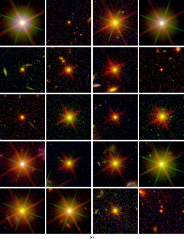
Figure 6. (a) log(log) color reproduction of a bright but unsaturated star image in the 10-band ERS color images in the GOODS-South field, using the same color balance prescription as in Figures 5(a) and (b). (b) Same for a "double" star. These images give a qualitative impression of the significant dynamic range in both intensity and wavelength that is present in these panchromatic ERS images. (c) log(log) color reproduction of the 20 ERS stars with the highest (≳3σ) proper motion, as discussed in Section 4.3.2 and Figure 4(c). Each image is 85 × 85 pixels or 765 × 765 on the side. The images used a similar color balance as in Figures 5(a) and (b), except that only the 2009 WFC3 UVIS filters F225W, F275W, and F336 are now in the blue gun, all the 2003 ACS BViz filters F438W, F606W, F775W, and F850LP are in the green gun, and the 2009 WFC3 IR filters F098M, F125W, and F160W are in the red gun. The RGB colors were further adjusted such that the proper motion between the Green 2003 ACS colors and the Blue+Red (or violet) 2009 WFC3 colors were maximally contrasted. In many cases, the proper motion is visible as an offset between the centroids of the Green and the Red+Blue images. For details, see the text.
Download figure:
Standard image High-resolution imageIn Figures 5(a) and (b), we used a log(log) stretch to optimally display the enormous dynamic range of the full resolution ERS color TIFF images. Figure 5(a) only displays the overlap between the 4 × 2 ERS UVIS mosaics, the GOODS v2.0 ACS BViz mosaics, and the 5 × 2 ERS IR mosaics. Each of the ERS mosaics are 8079 × 5540 pixels in total, but only about 6500 × 3000 pixels or 975 × 45 or 43.875 arcmin2 is in common between the UVIS and IR mosaics and shown in Figures 5(a) and (b). The area of the individual UVIS mosaics used in each of the UV–optical galaxy counts of Section 7 is substantially larger than this, but the total usable area of the IR mosaics is comparable to the area shown in Figure 5(a).
Figure 5(b) (see Appendix B.1) shows a zoom of the 10-band ERS color image, illustrating the high resolution available over a factor of 10 in wavelength, the very large dynamic range in color, and the significant sensitivity of these few orbit panchromatic images. Further noteworthy objects in the images are discussed in Appendix B.1 below.
4.3.2. Astrometric Quality of the ERS Mosaics
To compare the astrometry of our WFC3 ERS catalogs to our catalogs derived from the GOODS ACS v2.0 images, we selected the WFC3 H band, because the geometrical distortion correction (GDC) was measured thus far in the F160W filter only (see Appendix A). Amongst the GOODS ACS v2.0 images, we select the z'-band filter as the closest in wavelength to compare the ERS F160W images to astrometrically, and because most faint ERS stars are expected to be red (see Section 5.5). The GDC of the ACS/WFC has been well measured and calibrated over time and as a function of wavelength (Maybhate et al. 2010; Anderson 2002, 2003, 2007), and so is not a major source of uncertainty in this astrometric comparison. The exposure-time averaged effective epochs of the GOODS v2.0 ACS/WFC mosaics are: 2002.7796 in F435W, 2002.9755 in F606W, 2003.6083 in F775W and 2003.7634 in F850LP, respectively. Due to a continued GOODS high-z SN search that lasted from mid 2002 through early 2005, the spread on these numbers is about one year, yielding possibly somewhat elongated ACS images for very high proper motion stars in each of the GOODS v2.0 image stacks. The effective time-averaged epoch for the WFC UVIS ERS data is JD 2009.6918 in F225W, F275W, and F336W with a spread of 2 days, while for the WFC3 IR channel images the effective epoch is 2009.7370 in F098M, F125W, and F160W with a spread of about one week. For the WFC3 ERS images, image elongation for high proper motion stars is thus not a concern. The effective (WFC ERS–GOODS v2.0) epoch difference to be used for proper motions derived from this comparison is thus (2009.7370–2003.7634) = 5.97 ± 1 years, where the dispersion is dominated by the GOODS ACS z'-band image spread of about one year.
Figure 4(c) shows the measured residual astrometric offsets in (R.A., decl.) for all 4614 ERS objects matched between our WFC3 H-band object catalog and our GOODS ACS/WFC v2.0 z'-band catalog, as well as their histograms in both coordinates for 4511 matched ERS objects classified as galaxies (black) and 103 ERS objects classified as stars (red). Best-fit Gaussians are also shown for each of the histograms. As discussed in Section 4.2, the WCS coordinate system in the FITS headers of the WFC3 ERS images was by definition brought onto the well established GOODS ACS v2.0 WCS. This was done by applying WCS offsets averaged over all ERS objects to the WFC3 FITS headers. The histograms and curves in Figure 4(c) show that this could be done with an accuracy of 0.32 ± 0.46 (m.e.) mas in R.A., and 0.10 ± 0.41 (m.e.) mas in decl., respectively, i.e., in general to within 0.5 mas both randomly and systematically. While residual errors in the WFC3 GDC are large (see Section 4.2 and Appendix A), for a large number of objects spread over all the ERS images these errors apparently average out well enough to establish the overall WCS coordinate system of both the ERS UVIS and IR mosaics onto the GOODS v2.0 ACS/WFC mosaics to within 0.4–0.5 mas on average.
For the 4511 ERS galaxies alone, Figure 4(c) shows that the residual WFC3 offsets compared to GOODS ACS v2.0 are ΔR.A. = –0.64 ± 0.47 (m.e.) mas and Δdecl. = +0.38 ± 0.42 (m.e.) mas, or at the 1.4 and 0.9σ level in R.A. and decl., respectively. For the galaxies, these ERS offsets are indeed statistically insignificant, although they are not exactly equal to zero, because the matching onto the ACS WCS was done including the ERS stars as well—before it was known what the optimal star–galaxy separation method would be. (Because the residual offsets for all ERS galaxies alone are within the 0.4–0.5 mas errors quoted above, no second iteration was done in bringing the WFC3 WCS system on top of the GOODS ACS v2.0 WCS system.)
In total, 21 out of the 103 ERS stellar candidates show proper motion at the ⩾3σ level in R.A. or decl., respectively, as shown by the green asterisks in Figure 4(c). In total, 37 out of the 103 ERS stellar candidates show proper motion at the ⩾2σ level, also shown in Figure 4(c). Only about five stars are expected at ⩾2σ for a random Gaussian distribution, and so the stellar (ΔR.A., Δdecl.) offsets have a non-Gaussian distribution, as shown by the histograms in Figure 4(c). Hence, proper motion allows us to confirm statistically about 32 out of the 103 stellar candidates in the ERS. As a consequence, ERS proper motions alone cannot prove that all our ERS objects classified as stellar are in fact Galactic stars. For this reason, we will also consider object colors in Section 5.5 as confirmation of the stellar classifications.
Statistically, proper motions do cause significant offsets in the average (ΔR.A., Δdecl.) distribution of the 103 ERS objects classified as stars (Figure 4(c)). For these stellar candidates, we find on average that ΔR.A. = 13.71 ± 3.34 (m.e.) mas, or 2.30 ± 0.56 mas yr−1, and Δdecl. = −12.04 ± 2.09 (m.e.) mas, or 2.02 ± 0.35 mas yr−1. These constitute 4.1σ and 5.8σ detections of the statistical proper motion of all 103 ERS stellar candidates. The KS probability that the stellar ΔR.A. values are drawn from same distribution as the ERS galaxy population is 9.8 × 10⁻⁵, while for the stellar Δdecl. values this probability is 11 × 10−5. Hence, average stellar proper motion is detected at high significance level for the sample of 103 ERS stellar candidates. This is a significant result, since the star–galaxy separation of Section 5.5 was done completely independent of any proper motion information. A further discussion of this result is given in Sections 5.6 and 6.
Figure 6(c) shows a log(log) color reproduction of the 20 ERS stars with the highest (≳3σ) proper motion (green symbols in Figure 4(c)). The images used a similar color balance as in Figures 5(a) and (b), except that only the 2009 WFC3 UVIS filters are shown in the blue gun, all the 2003 ACS BViz filters were used in the green gun, and all the 2009 WFC3 IR filters in the red gun. The proper motion of these stars is best visible as significant centroid-displacements between the Green 2003 ACS colors and the Blue+Red (or violet) 2009 WFC3 colors (one has to magnify the PDF figure to best see the significant central green-to-white-to-orange displacement).
4.3.3. The Panchromatic ERS PSFs
Figure 6(a) shows a full color reproduction of a stellar image in the 10-band ERS color images in the GOODS-South field, and Figure 6(b) shows a "double" star. These images give a qualitative impression of the significant dynamic range in both intensity and wavelength that is present in the ERS images. Figure 7(a) shows images in all 10 ERS filters of an isolated bright star that was unsaturated in all filters, and Figure 7(b) shows its 10-band stellar light profiles. Table 2 lists the stellar PSF FWHM values in the 10 ERS bands. These include the contribution form the OTA and its wavefront errors and the specific instrument pixel sampling.

Figure 7. (a) Stellar images, and (b) Stellar light profiles in the individual 10-band images. Note the progression of the PSF size with wavelength, as discussed in Section 4.3.2.
Download figure:
Standard image High-resolution imageTable 2 and Figure 7(b) show the progression of the HST PSF (λ/D) with wavelength in the 10 ERS filters. Table 2 implies that the larger pixel values used in the multidrizzling of Section 4.2.2 indeed add to the effective PSF diameter. Table 2 also shows that that HST is diffraction limited in V band and longward, while shortward of V band, the PSF FWHM starts to increase again due to mirror micro-roughness in the ultraviolet. At wavelengths shorter than the V band, HST is no longer diffraction limited, resulting in wider image wings, and a somewhat larger fraction of the stellar flux visible outside the PSF core. The "red halo" at λ ≳ 0.8 μm is due to noticeable Airy rings in the stellar images in the WFC3 IR channel, and the well known red halo in the ACS z band (Maybhate et al. 2010) has an additional component from light scattered off the CCD substrate. Details of the on-orbit characterization of the WFC3 UVIS and IR PSFs are given by Hartig (2009a, 2009b).
4.3.4. The 10-band ERS Area and Depth
Table 1 summarizes the exposure times and the actual achieved depth in each of the observed ERS filters, while Table 2 also lists the effective area covered in each filter mosaic at the quoted depth.
The histograms of Figures 8(a)–(c) give the cumulative distribution of the maximum pixel area that possesses a specified fraction of total orbital exposure time. These effective areas must be quantified in order to properly do the object counts in Sections 6 and 7. After Multidrizzling the ERS mosaics in the UV and IR, these effective areas were computed from the weight maps, which include the total exposure time, and the effects from CR rejection, dithering, and drizzling. Figure 8(a) shows that about 50 arcmin2 of the UV mosaics has ∼80% of the UVIS exposure time, or ∼90% of the intended UV sensitivity. For reference, one 0090 pixel could be composed of 5.2 native WFC3 UVIS pixels times the number of exposures on that portion of sky. Due to overlapping dithers (see Figure 3), some pixels have more than the total orbital exposure time contributing to their flux measurement. The histograms of Figure 8(b) give the same information as Figure 8(a), but for the six GOODS v2.0 mosaic tiles in BViz that overlap with the ERS. Figure 8(c) gives the same information as Figure 8(a), but for the ERS mosaics in the IR. About 40 arcmin2 has ∼80% of the exposure time in the ERS IR mosaics, or ∼90% of the intended IR sensitivity. The overall WFC3 UVIS–IR sensitivity is 9%–18% better than predicted from the ground-based thermal vacuum tests (see Section 2.4 and Figure 2), and so in essence 100% of the intended ERS exposure time was achieved over the 50 arcmin2 UVIS images and the 40 arcmin2 IR images.

Figure 8. (a) Cumulative distribution of the maximum pixel area that has the specified fraction of total orbital exposure time in each ERS UVIS mosaic. These effective areas must be quantified in order to properly do the object counts in Figure 11(a). (b) Same as Figure 8(a), but for the GOODS v2.0 mosaics in BViz. (c) Same as Figure 8(a), but for the ERS mosaics in the WFC3 IR filters.
Download figure:
Standard image High-resolution image5. CATALOG GENERATION FROM THE 10-BAND ERS MOSAICS
5.1. Object Finding and Detection
All initial catalogs were generated using SExtractor version 2.5.0 (Bertin & Arnouts 1996). In general, these catalogs were generated SExtractor's single image mode for each ERS filter separately, so that the object finding could be done using the total object flux from each ERS filter independently, as is required when determining the star counts (Section 6) and the galaxy counts (Section 7). SExtractor was only used in its dual image mode to generate the additional catalogs that were used exclusively to make the color–color diagrams in Section 5.6 to confirm our star–galaxy separation procedure, using the H band as the detection image. As stated in Section 4.2.1, the ACS B-band image was used as the detection image to get an optimal object definition in the UVIS filters for reasons explained in detail here.
It was necessary to change the parameters in SExtractor to handle the UVIS images slightly differently than the ACS/WFC and WFC3/IR ones. This is due to several factors, both cosmetic and physical. The major difference is that galaxies appear much smoother in the IR and more clumpy in the UV, which occurs due to the specific distribution of their young and old stellar populations as well as their dust (see Windhorst et al. 2002 for a discussion of this effect for all Hubble types). Hence, star-forming regions in well-resolved galaxies can be deblended into separate objects by SExtractor if the deblending is overly aggressive. Fortunately, most of these intermediate-redshift galaxies are not bright in the observed UV, causing the UVIS fields to appear rather sparse, and making deblending a minor issue.
The UVIS images have a less uniform background (∼10%–15% of sky), which as discussed in Section 4.1.1 can possibly be improved, when accurate on-orbit UVIS sky flats have been accumulated over time. For these reasons, we adopted a seemingly low threshold for object detection with SExtractor, requiring 4 connected pixels that are 0.75σ above the background in the UV. Due to the clumpy nature of the ERS objects in the UV, we convolved the UVIS image with a Gaussian kernel of FWHM of 6.0 pixels for the object detection phase only. The deblending parameter, DEBLEND_MINCONT, was set to 0.1, to assure that real objects were not overdeblended. It should be emphasized that object crowding is not an issue in these medium depth UV images (e.g., Windhorst et al. 2008), so that the use of a larger SExtractor convolution filter, a lower SB-detection threshold, and less object deblending is fully justified. The 6.0 pixel Gaussian convolution kernel improves the SB sensitivity by ∼2 mag, given that the low-level UV sky gradients occur over much larger spatial scales than the typical faint galaxy sizes (see Sections 4.1 and 5.5). Together with the fact that the UVIS catalogs were made with SExtractor in dual image mode—using the much deeper ACS B-band image as the detection image, as described above—avoids excessive deblending of the very clumpy UV objects, which limits the number of spurious UV objects detected, as shown in the discussion of the ERS catalog reliability in Section 5.3.
The SExtractor input parameters for the ACS images and WFC3/IR images were the same. The detection threshold was set to 1.5σ, again requiring 4 connected pixels above the threshold for catalog inclusion. The convolution filter was a Gaussian with FWHM of 3.0 pixels, and DEBLEND_MINCONT was set to 0.06. For all 10 bands, the appropriate weight maps (see Section 4.2.2) were used in order to correctly account for image borders (Figure 3), as well as to properly characterize the photometric uncertainties and the effective areas for each mosaic (see Figures 8(a)–(c)).
5.2. Object Extraction
Two post-processing steps were taken to clean the catalogs of residual artifacts. First, due to the relatively small number of exposures per ERS filter, there were residual cosmic rays at the borders of the dither patterns, and in the chip gaps. These were cleaned by masking out all objects in regions where the number of exposures was less than three. Therefore, the total area coverage in each filter (Table 2 and Figures 8(a)–(c)) is slightly different. Second, SExtractor will detect the diffraction spikes of bright point sources. These are removed by searching for bright objects with FWHM near the size of the PSF and searching for surrounding objects in the catalog that are both highly elongated and oriented radially outward in sets of four from that compact object. Since the number of bright stars is not large (see Section 4.3.2 and figures therein, Sections 5.5 and 6.1), this is only a minor correction to the catalog, and only a few dozen diffraction spikes were found by SExtractor and removed in this way.
Magnitudes were all measured on the AB scale using the most current zero points available on the WFC3 Web site, which are listed in Table 2. Both Petrosian (1976) magnitudes were measured using a Petrosian factor of 2.0, and Kron (1980) magnitudes were measured using a Kron factor of 2.5 (SExtractor parameter MAG_AUTO). For the galaxy counts in Section 7.2, Kron magnitudes were used, because the correction to total magnitude—preferably using a Sersic extrapolation—is less than that typically required for a Petrosian magnitude. Within the errors, the Kron and Sersic based number counts are indistinguishable (Hill et al. 2011). The total magnitude errors in the ERS as a function of total AB magnitude were determined from the SExtractor errors in each filter, which are a combination of the MultiDrizzle RMS-map errors and the image shot noise.
5.3. ERS Catalog Reliability
To test the reliability of ERS object catalogs, we performed the negative image test (cf. Yan & Windhorst 2004). In brief, all 10 ERS mosaics were multiplied by –1.0, and then SExtractor was run with exactly the same parameters as the object finding procedure in Sections 5.1 and 5.2. This test showed that our ERS catalog generation was conservative due to the combination of several factors. These include drizzled the larger mosaic pixel size of 0090, the requirement of four connected pixels above the detection threshold, and the sizes of the Gaussian filters applied in the object detection phase. The choice of the SExtractor parameters listed in Sections 5.1 and 5.2 were determined by trial and error to create the most reliable catalogs at each wavelength.
In fact, these SExtractor parameter settings yielded no plausible spurious detections when it was run on the 10 negative ERS images. In total, only six negative "objects" were found, but these were all on the image borders, and the real ERS object catalogs were similar cleaned of such border defects. If the noise in the ERS images were completely Gaussian, then at the ≳5σ detection limit we would expect that 2.9 × 10⁻⁷ of the 6500 × 3000/4 independent ERS pixels (see Figure 5(a)) would yield a bogus object, or ∼1.4 bogus object in the combined 10-band catalog (the grand union) of 22,000 ERS objects. This is consistent with no convincing bogus objects found in the 10 negative ERS images after discarding the image borders. This exercise shows that at the 5σ 50% completeness level (see also Figure 9 below), our ERS object catalogs are ≳99.97% reliable. In astrophysical data samples, a compromise always has to be sought between sample reliability and sample completeness, while ideally maximizing the sum of the two (Windhorst et al. 1984a). The reason we choose here to have essentially 100% reliable catalogs—at the expense of some catalog incompleteness below—is the existence of the deeper optical–near-IR ACS and WFC3 images in the HUDF (Beckwith et al. 2006; Bouwens et al. 2010b; Yan et al. 2011b) in the BVizYsJH filters. These images made digging deeper into the ERS image noise unnecessary. Instead, the faint end of the galaxy counts at AB ≳ 26–27 mag in Section 7 will be derived in BVizYsJH from these HUDF images, which is in roughly the same direction of the sky.

Figure 9. Panchromatic completeness functions of the number counts in the panchromatic ERS images at the 5σ (red) and 10σ (blue) detection levels of total object magnitudes. These were derived by Monte Carlo insertion of faint point-like objects into the ERS images, and plotting the object recovery ratio as a function of total magnitude. At the ≳5σ level, the ERS is more than 50% complete at levels fainter than AB ∼ 26 mag for the WFC3 UVIS images, fainter than AB ∼ 27 mag for the WFC3 IR images, and substantially fainter than AB ∼ 27 mag for the deeper multi-year GOODS ACS v2.0 images (see Table 1).
Download figure:
Standard image High-resolution image5.4. ERS Catalog Completeness
Figure 9 shows the sample completeness functions of the 10-band ERS images. These were derived by Monte Carlo insertion of faint point sources into the ERS images, and plotting the object recovery ratio as a function of total magnitude. Most faint galaxies observed by HST are slightly resolved at the HST diffraction limit (e.g., Cohen et al. 2003; Hathi et al. 2008; Windhorst et al. 2008), so that for faint galaxies these limits are slightly brighter than for point sources, as discussed in Section 7.2 and shown in Figure 10(a).
In summary, the WFC3 UVIS images are ∼50% complete for point-like objects with ≳5σ detections in total flux for AB ≃ 26.3 mag in F225W, AB ≃ 26.4 mag in F275W, and AB ≃ 26.1 mag in F336W. The WFC3 IR images are ∼50% complete to AB ≃ 27.2 mag in F098M, AB ≃ 27.5 mag in F125W, and AB ≃ 27.2 mag in F160W, as listed in Table 1. The multi-year GOODS ASC/WFC v2.0 images in BViz are substantially deeper than this, and reach AB ≳ 27.5 mag in general. The actual star counts in Section 6 appear indeed complete to roughly these limits in the UV, but to slightly brighter limits in the IR due to the increasing object confusion of red stars with faint red background galaxies (see the figure in Section 5.5).
The actual UV galaxy counts in Section 7.2 turn over at a level rather close to the above UVIS point-source sensitivity limits. This is due to the generally more compact nature of the ERS objects, and the extremely faint zodiacal sky background in the UV. In the IR, the galaxy counts turn over at levels a little brighter than the 5σ point-source sensitivity limits listed in Table 2. This is due to the higher zodiacal sky-background values in the near-IR (see Table 2), combined with their somewhat larger sizes at the longer wavelengths (Section 5.5 and figures therein; see also Windhorst et al. 2002), even though faint red field galaxies selected in YsJH are in general still rather compact. Object confusion at these flux levels is relatively modest, especially at the HST diffraction limit, although natural confusion—which due to the intrinsic object sizes and not the instrumental PSF FWHM—becomes increasingly important at fainter fluxes (AB ≳ 25 mag; e.g., Windhorst et al. 2008).
In summary, the point-source sensitivity of our ERS catalogs is described by the simulations in Figure 9. The corresponding 50% point-source completeness limits are listed in Table 1. The actual observed panchromatic star counts (Section 6.1 and figures therein) are complete to roughly the 5σ limits of Figure 9 in the WFC3 UVIS filters, and to the 10σ limits of Figure 9 in the ACS BViz and WFC3 IR filters.
Rather than repeating the object simulations of Figure 9 to assess the actual completeness limits for the slightly extended galaxies (see Section 5.5 and figures therein), in Section 7 below we take a different and more empirical approach of determining the ERS incompleteness for faint galaxies by directly comparing the panchromatic ERS galaxy counts to AB ≲ 25.5–27 mag to the galaxy counts in the much deeper, but adjacent HUDF field. Since the effects of cosmic variance are relatively small over the 4' separation between the ERS and HUDF fields (see Section 7 and Figure 3), this comparison directly shows that the ERS catalogs are approximately ≳50% complete for samples of compact galaxies (see Section 5.5) to flux levels that are approximately 0.5–1.0 mag brighter (from the UVIS to the IR) than the ERS stellar samples in the same filters.
5.5. Star–Galaxy Separation in the ERS Mosaics
Stars and galaxies were separated as follows. In each filter, the stellar locus was defined as shown in the usual plot of the object FWHM versus total AB magnitude (e.g., Cohen et al. 2003). Figure 10(a) illustrates our star–galaxy separation procedure used for the 10-band ERS images. Objects with FWHM < PSF FWHM (from Table 2) are image defects, bad pixels, and some remaining CRs. Hence, objects to the left of the black vertical lines plotted at FWHM ≃ 007–015 are smaller than the PSF, and are discarded. Objects in the thin vertical filaments immediately larger than this are stars (plotted as thin reds dots in Figure 10(a)), and they in general have PSF FWHM ≲ FWHM ≲ (1+ ) × PSF FWHM, where 0 ≲ <1. Figure 10(a) shows that ERS stars straddle the instrumental PSF FWHM to AB ≃ 27 mag. Objects to the right of the black dashed slanted lines are galaxies, and they in general have FWHM ≳ (1+) × PSF FWHM, where "1+" is a weak function of total S/N, as shown by the two solid slanted lines in each of the panels in Figure 10(a).

Figure 10. (a) Panchromatic star–galaxy separation in the 10-filter ERS images. Plotted are object total AB magnitude vs. SExtractor image diameter FWHM (FWHM ≃ twice its half-light radius). Objects with image diameter ≲0.9 × PSF FWHM—where the PSF FWHM (≃007–015) is from Table 2—are image defects (black dots). Objects in the thin vertical filaments (red dots) immediately larger than this are classified as stars. ERS stars were defined to be those objects that resided in this red area in at least 3 out of 10 ERS filters. Objects to the right of the full-drawn slanted lines are galaxies (black dots). The star–galaxy separation becomes less reliable for fluxes fainter than AB ≃ 26–27 mag in UVBVizYsJH, respectively. Details are discussed in the text. (For best display, please zoom in on the full-resolution version of this image, which is available on http://www.asu.edu/clas/hst/www/wfc3ers/ERS2_gxysv4ln.tif.) (b) The (i − z) vs. (B − V) color–color diagram in the GOODS BViz filters for all ERS galaxies (black dots) and stars (red and green asterisks). These are compared to the Pickles (1998) model stellar SED library (blue squares), which range in spectral type from O5V to M7V, and also show the giant branch models up to type M7III. The observed ERS stellar colors are shown with their 1σ error bars. Only stars with combined color errors along each axis ≲0.5 mag are plotted. Green asterisks mark ERS stars with proper motion established at the ⩾2σ level.
Download figure:
Standard image High-resolution imageNext, all 10 independent ERS object catalogs—each with their independent star–galaxy separation and photometry—were merged by astrometric cross-matching. In order to maximize the 10-band information, we considered an object to be a star if it was classified as stellar in at least 3 out of 10 ERS filters. This provides robust stellar classifications, perhaps to fainter limits than can be done in single filter alone.
From Figure 10(a), we can see that the stars separate out well from the galaxies to about AB ≃ 25.5–26.0 mag, and somewhat fainter in the ACS BViz filters and the WFC3 IR filters. To these flux levels, the star counts follow a power law rather well, as shown in Section 6.1. The choice to require an object to be classified as a star in three filters—as opposed to all 10 filters—was made because stars can be either very red or sometimes very blue, and so stars are often not detected in all 10 ERS filters. Also, we are merging the data from three different HST instruments and detectors (WFC3 UVIS CCD, ACS/WFC CCD, and the WFC3 IR detector), so subtle PSF and sampling differences between these instruments can lead to the misclassification of a faint star in some of the 10 ERS filters, depending on its color. Since brighter stars are always seen at least in three (adjacent) ERS filters, we require all of the fainter stars to be classified as stellar in at least three of the ERS filters as well.
5.6. Confirmation of Star–Galaxy Separation: Proper Motion and Stellar Colors
As shown in Section 4.3.2 and Figure 4(c), all ERS objects together—which are ≳97.8% galaxies—allowed us to bring the WFC3 UVIS and IR coordinate system on average on top of the ACS WFC WCS to within 0.4–0.5 mas in both R.A. and decl. After having done this, the 4511 ERS objects classified as galaxies show indeed no significant residual motion over 5.97 years. However, for all 103 ERS objects classified as stars, an average proper motion of 2.30–2.02 mas yr−1 was detected at the 4.1σ–5.8σ level in R.A. and decl., respectively (see Section 4.3.2). For at least 32 out of the 103 ERS stars, this proper motion was discovered individually at the ⩾3σ level (see Figure 4(c)). The total average proper motion of all 103 ERS stars on the sky is 3.06 mas yr−1, summed in quadrature over the R.A. and decl. proper motions. The mean error is 0.66 mas yr−1, which amounts to a 4.6σ detection of the overall ERS stellar proper motion. The dispersion on this number in Figure 4(c) is 6.70 mas yr−1. We will interpret these numbers in more detail below. In conclusion, while ERS proper motions alone cannot confirm that all our ERS objects classified as stellar are in fact Galactic stars, average stellar proper motion is detected at high significance level for the entire sample of 103 ERS stellar candidates, making it in retrospect likely that most of these are in fact Galactic stars.
The ERS colors in Figure 10(b) are more conclusive in supporting our ERS star–galaxy separation procedure a posteriori. Figure 10(b) shows the (i − z) versus (B − V) color–color diagram in the GOODS filters, where all ERS objects have the highest S/N (see Figure 9). ERS objects classified as galaxies as shown as black dots, and ERS objects classified as stars with green or red asterisks. Green asterisks mark ERS objects that show proper motion at the ⩾3σ level in Figure 4(c) (see Section 4.3.2). The (i − z) versus (B − V) colors are compared to the Pickles (1998) model library SEDs (blue squares), which range in spectral type from O5V–M7V, and also show giant branch models up to M7III. The observed ERS stellar colors are shown with their 1σ error bars. Only stars with combined color errors along each axis ≲0.5 mag are plotted. It is clear that within the errors, most stellar ERS objects have colors of K–M type main-sequence stars, although there are a few ERS stars with color as blue as BV–GV types.
There are about 20 ERS stars in the color range 0 ≲ (B − V) ≲ 1.4 mag with (i − z) colors ≳0.3 mag redder than the Pickles (1998) main sequence. At least eight of these also have significant proper motion at the ≳3σ level, and are thus real Galactic stars. All 20 objects significantly redder than the Pickles (1998) main sequence were inspected by eye and correlated with other data. Three have VLT redshifts: one is a Seyfert galaxy at z = 1.031 in a group with similar spectroscopic redshifts, the other a compact elliptical at z = 0.251 next to a very faint stellar object, and the third is a stellar object next to an object at z = 2.217 with a neighbor at a similar redshift. The latter two stellar objects also have significant proper motion, and are likely real Galactic stars that are very close to an extragalactic object whose VLT redshift was actually measured.
Thus at least 17—and likely 19—of these 20 ERS stars with colors significantly redder than the Pickles (1998) main sequence have either significant proper motion and/or clear stellar morphology. Many of these appear to be stars that were unavoidably saturated in the ERS images. Because both their colors are ≳0.0 mag—they have higher ADU in i band than in z band, and in V band than in B band—given the ACS/WFC QE curve. Hence, their measured (i − z) flux will be too red, and their (B − V) color slightly too blue. Since these stars are saturated in nearly every ACS exposure, more accurate colors cannot be determined with the current mosaics, and their appearance above the Pickles (1998) main sequence does thus not rule them out as stars. Some of the reddest stars well away from the Pickles (1998) main sequence could be asymptotic giant branch stars with surrounding dust shells that could considerably redden their (B − V) and (i − z) colors significantly.
We also need to address how many of the stellar objects that are within the errors consistent with the Pickles (1998) stellar main sequence could be compact background galaxies. Figure 10(b) shows that the (i − z) versus (B − V) color space of zero-redshift stellar SEDs overlaps somewhat with the colors of intermediate-redshift galaxies, which largely occupy the region (B − V) ≲ 1 mag and (i − z) ≳ 0.15 mag. This is a limitation of the current color confirmation of the stellar ERS candidates. Only multi-parameter 10-band SED fitting of all ERS objects can address this issue more fully, which we will address in a future paper (Cohen et al. 2011). However, the available VLT spectra can give us some idea.
Among the 103 objects classified as ERS stars, many would have been bright enough to have been included in the VLT redshift survey, which is complete to AB ≲ 24 mag, but covered objects as faint as AB ≲ 25 mag. Among the 103 stellar ERS objects, 11 appear to be compact extragalactic objects confirmed to have VLT redshifts z>0. One of these is a quasar with an underlying early-type galaxy at z = 0.734.
In summary, this detailed study in Figure 10(b) confirms that at least 90–92 of the 103 stellar ERS objects have either significant proper motions (Figure 4(c)), stellar colors consistent with the Pickles (1998) main sequence (Figure 10(b)), and/or are not extragalactic objects with VLT redshifts z>0. Conservatively, we can thus conclude that our ERS stellar objects are indeed Galactic stars with ≳87% reliability. This provides a posteriori confirmation that our ERS star–galaxy separation method of Section 5.5—which was based on measured effective image diameters only (Figure 10(a))—is indeed valid. This then also means that we may consider the statistical proper motions of all ERS stars in Figure 4(c), to investigate if the implied average proper motion shows us something interesting about Galactic structure of very faint stars at high Galactic latitude (the GOODS-South field has bII = −54°). We discuss this in Section 6 in more detail.
As a final remark, ideally one would like the star–galaxy separation procedure to also include accurate fits of a library of (redshifted) SEDs to the 10-band ERS object photometry, and so help decide whether an object is most likely a zero-redshift star or a redshifted galaxy. This is beyond the scope of the current paper, and is pursued by Cohen et al. (2011) for the ERS stars and galaxies separately. This paper will also attempt to do a stellar + power-law AGN SED fits to all ERS objects, including on a pixel-to-pixel basis. This procedure will also provide better estimate of the AGN contamination of the ERS sample, rather than relying on the presence of weak point-like components in the ERS images alone. Suffice to say here that in Figure 10(b) most ERS stars have colors consistent with the stellar main sequence, so that contamination of our stellar ERS objects by weak AGN or other compact extragalactic objects is likely small. This is confirmed by the high proper motion stars in Figure 10(b), which have statistically the same color distribution as the stellar ERS objects without measurable proper motion.
6. RESULTS ON ERS STARS
6.1. The Panchromatic ERS Star Counts to AB ≃ 26 mag
Figure 11(a) shows the differential panchromatic star counts in the 10-band ERS images. The star–galaxy separation breaks down at fluxes AB ≳ 26 mag in BVizYsJH. However, for AB ≳ 22 mag galaxies outnumber stars by a large margin, so the more uncertain star–galaxy separation for AB ≳ 26 mag will not affect the quality of the galaxy counts. The star counts, of course, become correspondingly harder to do for AB ≳ 25 mag, and so in Section 6.2 and Figure 10(b) additional criteria such as colors and proper motion were used to confirm faint stars at higher confidence.

Figure 11. (a) Differential panchromatic star counts (red asterisks) and differential panchromatic galaxy number counts in the ERS images (black dots), with the optimized star–galaxy separation from Figure 10(a). All 10 ERS filters are shown in units of object numbers per 0.5 mag deg−2, but in the three bluest filters (F225W, F275W, and F336W) some of the brightest bins were doubled to 1.0 mag in width to improve statistics. The solid black line in the F850LP panel are the spectroscopic star counts from the HST PEARS ACS grism surveys of Pirzkal et al. (2009), which are in good agreement with our F850LP star counts. (b) ERS Star count slope (filled circles) versus observed wavelength in the flux ranges AB ≃ 19–25.5 mag for the three UV WFC3 filters, AB ≃ 16–26 mag for the GOODS/ACS BViz filters, and AB ≃ 15–25 mag for the three WFC3 IR filters, respectively. The faint end of the Galactic star count slope is remarkably flat at all wavelengths from the mid-UV to the near-IR, with best-fit power-law slopes in general of order 0.03–0.20 dex mag−1. The two bluest points at 153 and 231 nm are from the GALEX star counts of Xu et al. (2005; open squares), which cover AB = 17–23 mag. The ERS counts at the shortest wavelength suffer from small number statistics and so are less reliable (see Figures 10(a) and 11(a)). For further details, see the text. (c) ERS Galaxy count slope (filled circles) vs. observed wavelength in the flux ranges AB ≃ 19–25 mag for the three UV WFC3 filters, AB ≃ 18–26 mag for the GOODS/ACS BViz filters, and AB ≃ 17–25 mag for the three WFC3 IR filters, respectively. The two bluest points at 153 and 231 nm are from the GALEX galaxy counts of Xu et al. (2005; open squares), which cover AB = 17–23 mag. The galaxy counts show the well known trend of a steepening of the best-fit power-law slope at the bluer wavelengths, which is caused by a combination of the more significant K-correction and the shape of the galaxy redshift distribution at the selection wavelength.
Download figure:
Standard image High-resolution imageThe solid black line in the F850LP panel of Figure 11(a) represents the spectroscopic star counts to AB ≃ 25 mag from the HST Cycle 14 ACS grism survey "PEARS" (Probing Evolution And Reionization Spectroscopically) of Pirzkal et al. (2009). Since for these objects we can use the low-resolution ACS G800L spectroscopic data as independent confirmation of their stellar nature, they have higher accuracy than the image-based star counts alone. The southern PEARS ACS grism survey was done over a similar sized area to the ERS, covering an overlapping portion of GOODS-S. Hence, it is encouraging that the Pirzkal et al. (2009) grism star counts, which are for spectral types of M0 and later, have the same slope as our direct-imaging ERS star counts in F850LP. The slightly different star count amplitude for the flux range 18 mag ≲ AB ≲ 25 mag is likely due to the fact that the spectroscopic sample was limited to later spectral types, where those grism classifications were most reliable. The good agreement in star counts between the two different survey methods confirms that—as far as faint stars are concerned—our star–galaxy separation is accurate to about AB ≃ 25 mag.
Figure 11(b) shows the ERS star count slope versus observed wavelength in the flux ranges AB ≃ 19–25.5 mag for the three UV WFC3 filters, AB ≃ 16–26 mag for the GOODS/ACS BViz filters, and AB ≃ 15–25 mag for the three WFC3 IR filters, respectively. The GALEX FUV and NUV points of Xu et al. (2005) are also plotted at 153 and 231 nm, and cover the flux range AB ≃ 17–23 mag, using primary color criteria to accomplish star–galaxy separation at the 4''–66'' FWHM GALEX resolution. The statistics of the star counts in the three bluest ERS filters (F225W, F275W, and F336W) are rather sparse (Figure 11(a)). As a consequence, our three bluest best-fit ERS power-law slope values are rather uncertain, as indicated by the larger error bars in Figure 11(b). The GALEX FUV and NUV star count points of Xu et al. (2005) are complete to somewhat brighter levels (AB ≃ 23–24 mag), but have much better statistics. As a consequence, the GALEX FUV and NUV star count slope points in Figure 11(b) have smaller error bars, and at the common wavelength of ∼230 nm they therefore carry larger weight than the ERS star count slope in the mid-UV.
Given these uncertainties, the Galactic star count slope at the faint end is remarkably flat at all wavelengths from the Balmer break to the near-IR, although it is rather poorly determined from the ERS data alone below the Balmer break. The values of the best-fit ERS power-law star count slope is in general of order 0.03–0.05 dex mag−1. Including the more accurate GALEX star count slope values at 150 and 230 nm, the panchromatic faint end of the star-count slope appears to be always in the range 0.03–0.20, i.e., at all ERS wavelengths the faint star-count slope remains well below Euclidean value of 0.6 dex mag−1. This shows that to a depth of AB ≃ 25–26 mag at all wavelengths in the range 0.2–2 μm, the ERS images readily penetrate through most of the thick disk of our Galaxy at these latitudes (bII ≃ −54°) in the direction of the Galactic anti-center (lII = 224°; Ryan et al. 2005; Beckwith et al. 2006). This trend was also seen in the red ACS imaging parallels of Ryan et al. (2005), and the red ACS GRAPES and PEARS grism observations of Pirzkal et al. (2005, 2009), respectively, each of which constrained the scale height of Galactic L and T dwarfs to about 300–400 pc.
In the bluest three WFC3 filters F225W, F275W, and F336W, the WFC3 ERS finds only 22, 18, and 27 faint stellar candidates, respectively. Most of the full sample of ERS stars have 10-band colors red enough to indicate Galactic halo K–M type stars and possibly a few L and T dwarfs, but a few of the faint stars are blue (see Section 5.6 and Figure 10(b)). The latter could be faint Galactic white dwarfs, though there were no UV detected stars that were not also seen in the ACS B band. The effective ERS UV stellar detection limit of AB ≃ 25 mag could trace a T = 2 × 10⁴ K white dwarf with an absolute magnitude in the range Mbol ≃ +15 to +10 mag (Harris et al. 2006) out to a distance of 1–10 kpc, respectively, assuming modest bolometric corrections. The faint stellar objects in the 10-band ERS data are obviously of great interest by themselves and will be studied in more detail in a future paper. An important lesson learned for UV observations of high-latitude fields is that there are so few UV bright stars, that one has to ensure that individual exposures are long enough in order to align and drizzle (or stack) them using faint galaxies. In the ERS UV images we did this using the cross-correlation technique, as explained in more detail in Appendix A.
6.2. The Nature of Faint ERS Stars from Proper Motion and Stellar Colors
Figure 10(b) suggests that the majority of ERS stars have red colors characteristic of faint red main-sequence stars. Their typical spectral type is in the range K0V–M5V with an average spectral type of ∼K5V. For these stars, the expected MV ranges from +5.8 to +12.3 mag with an average of MV ∼+8 mag. With the flat ERS star count slope of Figure 11(a), the average ERS star has an AB magnitude of ∼23 mag, while the ERS stellar detection limit is AB ≲ 26 mag. Hence, the average faint red ERS star will be at a distance of about R ≃ 10 kpc from the Sun. The direction of the GOODS-South field at R.A. = 03h32m39s, decl. = −27°47'291 is in the Southern Galactic hemisphere, about 54° below the plane of the Milky Way, and in the general direction of the Galactic anti-center. Stars in this direction at ∼10 kpc distance from the Sun will thus be bulge and disk stars ∼8 kpc below the Galactic plane, i.e., well below the outer Orion arm of the Galaxy. At this distance, the above average ERS proper motion of 3.06 ± 0.66 mas yr−1 amounts to an average stellar tangential velocity of ≲145 ± 31 km s−1 (m.e.). These stellar velocities and their dispersion are in part due to the projected solar motion in the sky—compared to the Galactic Local Standard of Rest—and in part due to the true space velocities of ERS stars in the Galactic bulge and disk. While a detailed discussion of the proper motion of ERS stars and its implication for Galactic structure is beyond the scope of the current paper, we will here briefly discuss how our ERS proper motion results compare to previous proper motion and radial velocity observations of the Galactic bulge and disk at intermediate to high Galactic latitude.
A proper motion study to V ≲ 22.5 mag at the North Galactic Pole by Majewski (1992) shows a systemic velocity of −120 km s−1 at the edge of the thick disk (z ≳ 5.5 kpc). Clarkson et al. (2008) show similar proper motion values at R∼ 5 kpc, but in Baade's window from multi-epoch HST/ACS images that are effectively complete to about I ≲ 21 mag given the more crowded images at low Galactic latitudes. Kinman et al. (2007) find that Galactic Blue Horizontal Branch stars with an average distance to the Galactic plane of z ≲ 8 kpc have zero galactic rotation and roughly isotropic velocity dispersions of 93–81 km s−1 in the tangential and z directions, respectively, or ∼123 km s−1 in the plane of the sky. Theoretical disk+bulge+halo models (Battaglia et al. 2005; Klypin et al. 2002) predict velocity dispersions at R∼ 5–10 kpc of 150 km s−1 for the Galactic bulge+thick disk components.
These values are very similar to the 145 km s−1 value implied from the average proper motion observed for our faint red ERS stars at relatively high Galactic latitude (bII = −54°). In other words, the Galactic (thick disk+bulge) velocity dispersion implied from our faint red ERS stellar proper motions is consistent with these previous observations and theoretical model predictions. It is worth noting, however, that these previous observations are based on high-resolution radial velocities and proper motions of Galactic stars with V ≲ 16 mag, or proper motions alone for stars with V ≲ 22.5 mag. Our ERS observations push this substantially fainter for proper motions at high Galactic latitudes, to flux levels (AB ≲ 25–26 mag) where high resolution spectroscopy cannot be done with current ground based facilities. Systematic proper motion studies of very faint stars at HST resolution at high Galactic latitudes thus have the potential to sample part of Galactic structure that is otherwise not easily accessible. This topic will be studied in further detail in a subsequent paper.
7. RESULTS ON GALAXIES IN THE ERS
7.1. The Panchromatic ERS Galaxy Counts to AB ≃ 26–27 mag
Figure 11(a) also shows the differential panchromatic galaxy number counts in the 10-band ERS images. No completeness corrections—as implied by Figures 9 and 10(a)—were applied to the faint end of the panchromatic ERS galaxy counts in Figure 11(a). Instead, to be conservative, the data points are not plotted in all panels of Figure 12 at the flux level where the counts clearly start to deviate from a best-fit faint-end power law (see Figures 11(a) and (c)) by more than 50%. This in general occurs 0.5–1.0 mag brighter than the 50% point-source completeness limits listed in Table 1, as derived from Figure 9.
Figure 11(c) shows the ERS galaxy count slope versus observed wavelength in the flux ranges AB ≃ 19–25 mag for the three UV WFC3 filters, AB ≃ 18–26 mag for the GOODS/ACS BViz filters, and AB ≃ 17–25 mag for the three WFC3 IR filters, respectively. The GALEX FUV and NUV points of Xu et al. (2005) are also plotted at 153 and 231 nm, and cover AB = 17–23 mag, again using primary color criteria to accomplish star–galaxy separation at the 4''–6'' FWHM GALEX resolution. The statistics of the galaxy counts in the three bluest ERS filters (F225W, F275W and F336W) are sparse (Figure 11(a)), and at the bright-end the ERS object definition and deblending is more complex given the sizes of the brighter objects (Figure 10(a)). As a consequence, the best-fit ERS galaxy count power-law slope values become somewhat more uncertain at the bluer ERS wavelengths (Figure 11(c)). The GALEX FUV and NUV galaxy counts of Xu et al. (2005) are complete to somewhat brighter levels (AB ≃ 25 mag), but have much better statistics than the ERS. Given the much larger size of the GALEX beam (4''–6'' FWHM), they do however suffer from more uncertain star–galaxy separation, which for GALEX needed to be done by using multi-color information as well (Baldry et al. 2010). At the longer GALEX wavelength, it may be harder to separate Galactic stars from low-redshift older galaxies using colors alone. As a consequence, the GALEX NUV count slope point in Figure 11(c) has a somewhat larger error bar at the common wavelength of ∼230 nm.
Given the above uncertainties in the GALEX and ERS UV galaxy count slopes, the galaxy counts show the well known trend of a steepening of the best-fit power-law slope at the bluer wavelengths, which is caused by a combination of the more significant K-correction and the shape of the galaxy redshift distribution at the selection wavelength. The galaxy count slope changes significantly from a ≳ 0.44 dex mag−1 at 0.23 μm wavelength to a ≃ 0.26 dex mag−1 at 1.55 μm wavelength. Hence, the galaxy counts have a slope flatter than the Euclidean value of a ≃ 0.6 dex mag−1. However, at wavelengths below 0.4 μm the UV galaxy counts are steeper than the a⩽ 0.4 dex mag−1 value required for their sky brightness integral to converge to a finite value, if they were to continue with this power-law slope for AB ≳ 27 mag. That is, the UV galaxy counts will have to turn over with a slope flatter than ⩽0.4 dex mag−1 for AB ≳ 27 mag. In Section 7.3 we will confirm that they indeed do so.
7.2. The Panchromatic Galaxy Counts for 10 mag ≲ AB ≲ 30 mag
Figures 12(a)–(j) show the galaxy number counts in the 10-band ERS images compared to a number of other panchromatic surveys at the bright end and at the faint end. At the bright end, we added the counts from the GAMA survey (Driver et al. 2009) in NUV+ugrizYJH, which cover AB = 10–21 mag (Xu et al. 2005; Hill et al. 2010). Details on the ground-based data obtained in the GAMA survey are given by Driver et al. (2009) and Hill et al. (2010). The GAMA survey also uses matched aperture Kron magnitudes, which are comparable to our total magnitudes used for the ERS.

Download figure:
Standard image High-resolution image
Download figure:
Standard image High-resolution image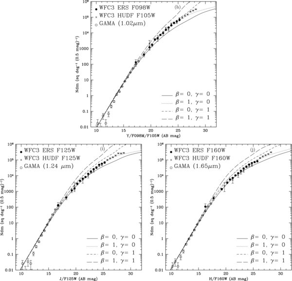
Figure 12. (a)–(c) Differential galaxy number counts for the entire flux range AB = 10–30 mag in the F225W (a), F275 (b), and F336W (c) filters. For comparison at the bright end, we added to the ERS number counts from Figure 11(a) the panchromatic GAMA survey (Driver et al. 2009) counts in NUV+ugrizYJH, which cover AB = 10–21 mag (Xu et al. 2005; Hill et al. 2010). At the faint end, we added the WHT U band and HDF-North and South F300W counts of Metcalfe et al. (2001), the deep LBT U-band counts of Grazian et al. (2009), as well as the deep HST STIS counts of Gardner et al. (2000). Best-fit luminosity and number density evolution models cover AB ≃ 10–30 mag (see Driver et al. 1998; Hill et al. 2010). (d)–(g) Differential galaxy number counts for the entire flux range AB = 10–30 mag in the F435W (d), F606W (e), F775W (f), and F850LP (g) filters. Further details are given in the caption of Figures 12(a)–(c) At the faint end, we also added the HUDF counts in BViz from Beckwith et al. (2006), which cover AB = 23–30 mag. (h)–(j) Differential galaxy number counts for the entire flux range AB = 10–30 mag in the F098M/F105W (h), F125W (i) and F160W (j) filters. Further details are given in the caption of Figures 12(a)–(c). At the faint end, we also added the HUDF counts from the Bouwens et al. (2010b) YJH data, as compiled by Yan et al. (2011b), which cover AB = 24–30 mag.
Download figure:
Standard image High-resolution imageThe GAMA star–galaxy separation procedure is quite different than for the ERS, since there is a significant potential for contamination by stars which dominate the number counts at brighter magnitudes (Figure 11(a)). The GAMA star–galaxy separation therefore uses the (rPSF–rmodel) parameter to determine how extended an object is, and also uses the well-defined stellar locus in the (g − i) versus (J − K) color–color diagram. Details of the star–galaxy separation methods used in the GAMA survey are given by Baldry et al. (2010).
At the faint end in Figures 12(d)–(j), we added the HUDF counts in BViz from Beckwith et al. (2006), which cover AB = 24–30 mag, and the HUDF counts from the Bouwens et al. (2010b) data in the F105W, F125W, and F160W filters (hereafter YJH), as compiled by Yan et al. (2011b), which cover AB = 24–30 mag. In the UV, we added the William Herschel Telescope (WHT) U-band counts and the HDF-North and South F300W counts as compiled by Metcalfe et al. (2001), the deep Large Binocular Telescope (LBT) U-band counts of Grazian et al. (2009), as well as the deep HST STIS UV counts of Gardner et al. (2000).
We note that the filter systems in the comparisons in each of Figures 12(a)–(j) are not quite identical, although they were chosen in every case to be as close as possible in wavelength (typically to within 0.1 dex). Hence where necessary, small but appropriate AB-mag offsets or color transformations were made between the filters and models used in each plot, following Metcalfe et al. (2001) or Windhorst et al. (1991). These corrections generally contain some color dependence. When applying them as a single AB-flux scale correction to a given survey can introduce uncertainties of order 0.1 mag in the flux scale used. Over the entire AB = 10–30 mag range shown in Figures 12(a)–(j), such ∼0.1 mag offsets would not be noticeable. However, for a detailed set of modeling in subsequent work, more subtle flux and color dependent corrections may need to be applied. This will be the subject of a future paper.
The error bars in each of the counts in Figures 12(a)–(j) are Poisson, and therefore do not include effects from cosmic variance. To increase the statistics where necessary at the bright end of each survey, bins were combined logarithmically using the local slope of the galaxy counts, following the prescription of Windhorst et al. (1984b). At the faint end, the counts are not plotted in Figures 12(a)–(j) fainter than the flux level where these are deemed complete. Based on Figures 9 and 11(a), this occurs in general where the counts turn over significantly within the statistical error bars. Hence, in principle, the panchromatic counts of Figures 12(a)–(j) should be comparable over the entire flux range AB ≃ 10–30 mag, except for the effects of cosmic variance. The latter is small for the panchromatic ∼116 deg2 GAMA survey, but it could be important for the other panchromatic survey areas plotted, such as the ERS and the HUDF which are both (disjoint) parts of GOODS-S, as well as the HDF-North (in GOODS-North) plus the HDF-South and various other ground-based surveys in the U band.
In the flux range where the panchromatic GAMA and HUDF counts in Figures 12(a)–(j) overlap with the panchromatic ERS counts, the agreement is in general quite good, except at the bright end of the ERS, which suffers from cosmic variance, and from the fact that the GOODS/ERS field was chosen to be devoid of objects much brighter than AB = 18 mag. As a consequence, the bright end of the ERS galaxy counts also suffers somewhat from incompleteness. The same is true for the bright end of the HUDF, which suffers similarly from cosmic variance and the avoidance of objects much brighter than AB ∼ 21–22 mag when that field was selected in early 2003 for the ultradeep HST survey. The HUDF is adjacent to, but does not overlap with the ERS area (see Figure 3). The HUDF galaxy counts in BVizYsJH are in good agreement with the ERS galaxy counts to the flux levels where the panchromatic ERS counts are considered complete (AB ≃ 26–27 mag in Figure 11(a)).
The good agreement between these various surveys also implies that the flux scales of the panchromatic ERS counts are approximately correct. Had one of the ERS filter zero points been off significantly (e.g., by more than 0.1–0.2 mag), we would have noticed this as a significant offset between the counts. Note this argument only holds for the counts at AB ≳ 20 mag, as these cover the same general area of sky in the GOODS-South field. Hence, cosmic variance likely affects these counts similarly over such scales (≲ 30%; Somerville et al. 2004).
7.3. Modeling the Panchromatic Galaxy Counts for 10 mag ≲ AB ≲ 30 mag
Figures 12(a)–(j) overplot simple galaxy evolution models by Driver et al. (1995, 1998), which have been updated for the current comparison with the ERS. Driver et al. (1995, 1998) and Cohen et al. (2003) provide further details of these models. In short, they use the best available local LF as a function of galaxy type, and K-corrections from the Bruzual & Charlot (2003) spectral evolution models, also as a function of galaxy type. The local galaxy LF then gets integrated with the WMAP year 7 (Komatsu et al. 2011) cosmological volume element to predict the number density of galaxies observed to the total-flux limit in each ERS filter. These models also include internal reddening as a function of galaxy type.
These models have been updated with the best available local panchromatic LFs in ugrizYJHK from the Millennium Galaxy Catalog survey by Hill et al. (2011), and in the UV they use the GALEX LFs of Robotham & Driver (2011). These LFs will be updated in future work with GAMA redshifts from the three-year Anglo-Australian Telescope survey that was concluded in 2010. Robotham et al. (2010) provide further details on the GAMA redshift survey. This GAMA data set is currently 99% redshift complete for rPetro ≃ 19.4 mag, and provides high-fidelity, matched-volume panchromatic LFs, which are essential to interpret the higher-redshift panchromatic ERS work.
Evolution of the faint-end LF slope is not yet included in these simple models, but the panchromatic local GAMA LFs automatically includes the well-known steepening of the local LF toward shorter rest-frame wavelengths, where the local LF is dominated by the more rapidly star-forming late-type galaxies (see Driver et al. 1998; Robotham & Driver 2011; Hill et al. 2011). The epoch-dependent galaxy redshift distribution is also not an input to these models, but can instead be inferred from the local LF as a function of type (e.g., Driver et al. 1996), the total constraints provided by the panchromatic galaxy counts (Figures 12(a)–(j)), the adopted K-corrections as a function of galaxy type, and the adopted evolutionary model parameters. These simple evolution models used are either a pure luminosity evolution (PLE) model with e(z) = 2.5 log[(1+z)β] and PLE exponent β, or a number density evolution (NDE) model with n(z) = no [(1 + z)γ] and NDE exponent γ, or a combination thereof.
Based on the currently available, best panchromatic local GAMA LFs, Figures 12(a)–(j) show for AB = 10–30 mag the PLE model prediction with PLE exponent β = 1 (dotted lines), the NDE model prediction with NDE exponent γ = 1 (short-dashed lines), or a combination of both models indicated by both parameters β = γ = 1 (long-dashed lines). The solid lines show in all cases the non-evolving model (β = γ = 0).
Over the entire flux range AB ≃ 10–30 mag, Figures 12(a)–(j) show that no single PLE model fits all the available galaxy count data, since there is not enough volume at high redshift to make any PLE model fit the high observed counts, especially in the visual to near-IR (Figures 12(d)–(j)). This means that one has to invoke NDE as well, i.e., β ≳ 1 and some modest amount of luminosity evolution for γ ≳ 0. The best models using these PLE or pure density evolution (PDE) prescriptions are either the β ≃ 1 or the γ ≃ 1 model. Figures 12(a)–(j) also shows that no single combined PLE+NDE model fits the panchromatic galaxy counts in all 10 bands simultaneously over the entire observed range AB ≃ 10–30 mag, not even with the best available panchromatic local LF from the GAMA survey (Hill et al. 2011).
In particular, Figures 12(d)–(j) show that at the faint end of the galaxy counts in YJH there exists a significant excess in observed object numbers compared to these simple models. This could be due to either an additional population of objects at high redshifts, or—more likely—due to lower luminosity objects at lower redshifts, and/or because some essential aspects are missing in these models. A detailed discussion of these possibilities is beyond the scope of the current paper, but the reader is referred to, e.g., Bouwens et al. (2010b), Yan et al. (2011b), and Wyithe et al. (2011) for a discussion of some of these possibilities.
More realistic galaxy evolution models would be ones in which the faint-end Schechter LF-slope α also evolves with redshift, as has been suggested by, e.g., Ryan et al. (2007) and Khochfar et al. (2007). In particular, the faint-end LF-slope α steepens significantly at higher redshifts, which was suggested by, e.g., Yan & Windhorst (2004), Ryan et al. (2007), Hathi et al. (2010), and Oesch et al. (2010b). One would like to compare our panchromatic ERS galaxy counts from 0.2 to 2 μm over the entire observed range AB = 10–30 mag (Figures 12(a)–(j)) to state-of-the-art hierarchical simulations that reach from z = 8 to z = 0, and properly fold star formation and stellar population evolution models with these ΛCDM simulations. Such models have been made, e.g., by Croton et al. (2006), de Lucia & Blaizot (2007), and Nagamine et al. (2005a, 2005b), and are discussed in further detail by, e.g., Kitzbichler & White (2007), Monaco et al. (2007), and Nagamine (2006). It is difficult for such models to predict reliable panchromatic galaxy counts from 0.2 to 2 μm that cover the entire observed range AB = 10–30 mag, because such simulations take a very large amount of computing time to cover the low-redshift regime (z ≲ 3), to cover the entire galaxy LF, and to let and them run all the way to z = 0. In addition, such models need to include increasingly complex physics with cosmic time, such as hierarchical merging and/or downsizing, feedback processes from SNe and AGNs, and how these processes changed the faint end and bright end of the galaxy LF, respectively, over cosmic time, as well as include the physics of dust. This will be the subject of a future paper that compares the observed panchromatic galaxy counts from 0.2 to 2 μm over the entire flux range AB = 10–30 mag to available hierarchical models.
For now, we conclude that the simple PLE+PDE models with the best available observed panchromatic local LF from GAMA can explain each of the 10-band counts for 10 mag ≲ AB ≲ 30 mag individually, but no single one of the simple PLE+NDE models can explain the counts over this entire flux range in all 10 filters simultaneously.
8. SUMMARY AND CONCLUSIONS
In this paper, we presented the new HST WFC3 ERS observations in the GOODS-South field. We presented the scientific rationale of this ERS survey and its data, the data taking plus data reduction procedures of the panchromatic 10-band ERS mosaics. We described in detail the procedure of generating object catalogs across the 10 different ERS filters.
The new WFC3 ERS data provide calibrated, drizzled mosaics in the UV filters F225W, F275W, and F336W, as well as in the near-IR filters F098M (Ys), F125W (J), and F160W (H) in 1–2 HST orbits per filter. Together with the existing HST Advanced Camera for Surveys (ACS) GOODS-South mosaics in the BViz filters, these panchromatic 10-band ERS data cover 40–50 arcmin2 at 007–015 FWHM resolution and 0090 Multidrizzled pixels to depths of AB ≃ 26.0–27.0 mag (5σ) for point sources and AB ≃ 25.5–26.5 mag for compact galaxies. The galaxy samples are ≳50% complete to these limits, and ≳99.97% reliable.
We also described the high quality star–galaxy separation made possible by the superb resolution of HST/WFC3 and ACS over a factor of 10 in wavelength to AB ≃ 25–26 mag from the UV to the near-IR, respectively, using proper motion and BViz colors to confirm the star–galaxy separation procedure, which has an overall reliability of ≳87% for stars. Our main science results are as follows.
- 1.We present the resulting Galactic star counts and galaxy counts in 10 different filters. From the ERS data, these could be accurately determined from AB ≃ 19 mag to AB ≃ 26 mag over a full factor of 10 in wavelength from the mid-UV to the near-IR.
- 2.Both the Galactic star counts and the galaxy counts show mild but significant trends of decreasing count slopes from the mid-UV to the near-IR over a factor of 10 in wavelength.
- 3.The galaxy count slope changes significantly from a ≃ 0.44 dex mag−1 at 0.23 μm wavelength to a ≃ 0.26 dex mag−1 at 1.55 μm wavelength, showing the well known trend of a steepening of the best-fit power-law slope at the bluer wavelengths. This is caused by a combination of the more significant K-correction and the shape of the galaxy redshift distribution at the selection wavelength.
- 4.We combine the 10-band ERS counts with the panchromatic GAMA counts at the bright end (10 mag ≲ AB ≲ 20 mag), and with the ultradeep HUDF counts in BVizYsJH and other available HST UV counts at the faint end (24 mag ≲ AB ≲ 30 mag). The galaxy counts are now well measured over the entire flux range 10 mag ≲ AB ≲ 30 mag over nearly a factor of 10 in wavelength.
- 5.We fit simple galaxy evolution models to these panchromatic galaxy counts over this entire flux range 10 mag ≲ AB ≲ 30 mag, using the best available 10-band local galaxy LFs from the GAMA survey (Hill et al. 2010), as well as simple prescriptions of luminosity and/or density evolution. While these models can explain each of the 10-band counts for 10 mag ≲ AB ≲ 30 mag individually, no single one of the simple PLE+NDE models can explain the counts over this entire flux range in all 10 filters simultaneously. Any more sophisticated models of galaxy assembly, including hierarchical merging and/or downsizing with or without feedback, need to at least reproduce the overall constraints provided by the current panchromatic galaxy counts for 10 mag ≲ AB ≲ 30 mag over a factor of 10 in wavelength.These surveys also emphasize the need for extending this work to levels fainter than AB ≳ 30 mag and at longer wavelengths, which the JWST will do for wavelengths in the range 0.6–28 μm after its launch after 2015. The unique abilities of WFC3 to do deep UV imaging will need to be explored fully before that time.
- 6.We show examples of interesting panchromatic faint galaxy structure in intermediate-redshift objects, including early-type galaxies with nuclear star-forming rings and bars, and/or weak AGN activity, and some objects of other unusual appearance.
The panchromatic ERS database is very rich in structural information at all rest-frame wavelengths where young or older stars shine during the peak epoch in the cosmic star formation rate (z ≃ 1–2) and constitutes a unique new HST data base for the community to explore in the future.
This paper is based on Early Release Science observations made by the WFC3 Scientific Oversight Committee. We are grateful to the Director of the Space Telescope Science Institute, Dr. Matt Mountain, for generously awarding Director's Discretionary time for this program. We thank Drs. Neill Reid, Ken Sembach, Ms. Tricia Royle, and the STScI OPUS staff for making it possible to have the ERS data optimally scheduled. We also thank WFC3 IPT and the GSFC WFC3 Project for their very hard dedicated work since 1998 to make this wonderful instrument work, and for their timely delivery of the essential hardware and software to make the acquisition and reduction of the new WFC3 data possible. We also thank the entire GOODS team and in particular Drs. Norman Grogin and Mauro Giavalisco for making the exquisite GOODS v2.0 mosaics available. We thank Drs. Norman Grogin and Paul Schmidtke for helpful discussions. We thank the referee for very thoughtful suggestions, which helped improve the presentation of this paper, and for prompting a more detailed study of the ERS stellar proper motions and colors, which we believe illustrates the multi-faceted promise of the ERS data.
Support for HST program 11359 was provided by NASA through grant GO-11359 from the Space Telescope Science Institute, which is operated by the Association of Universities for Research in Astronomy, Inc., under NASA contract NAS 5-26555. R.A.W. also acknowledges support from NASA JWST Interdisciplinary Scientist grant NAG5-12460 from GSFC. H.Y. is supported by the long-term fellowship program of the Center for Cosmology and AstroParticle Physics (CCAPP) at The Ohio State University.
We thank the STS-125 astronauts for risking their lives during the Shuttle Servicing Missions SM4 to Hubble, and for successfully installing WFC3 into HST in 2009 May. We dedicate this paper to the memory of the STS-107 Columbia Shuttle astronauts and of Dr. Rodger Doxsey, who during their lives contributed so much to the Space Shuttle and the Hubble Space Telescope projects.
APPENDIX A: THE WAVELENGTH-DEPENDENT UVIS GEOMETRIC DISTORTION CORRECTION
Given the issues related to the GDC discussed in Section 4.2.2, it was apparent that some astrometric residuals remained—at the level of ≲2–3 Multidrizzled pixels—that were a function of position across both UVIS detectors, after the shifts and rotations had been removed. A worst case is shown in the lower panel of Figure 4(a). These residuals were apparent between the three UVIS filters, as well as relative to the GOODS astrometric frame. At the time of the data reduction, the best available Instrument Distortion Coefficients (IDCtab's; file t982101i_uv_idc.fits)—which are used for the GDC—had been created using the WFC3 SMOV F606W data alone30. This GDC did not yet include any wavelength-dependent distortion terms, though these will be measured during Cycle 18 or beyond31, and distributed to the community by the WFC3 instrument team. Since our WFC3/UVIS data are all taken at wavelengths below 3500 Å, it is likely that the remaining astrometric residuals are indicative of the absence of these color-dependent terms in the currently existing GDC tables. The wavelength-dependent terms of the GDC come from the different index of refraction of the glass optics and filters in the UVIS channel of WFC3. This is in addition to the first- to third-order geometric distortion coefficients, which results from the CCD tilt (which was necessary to minimize internal reflections), and from other reflective optics, and are therefore largely wavelength-independent.
The ultimate goal of the UVIS part of the WFC3/ERS is to create images in F225W, F275W, and F336W filters at the same pixel scale (0030 per pixel) and astrometric grid as the GOODS ACS images (Giavalisco et al. 2004) of the same portion of the GOODS-South field. As discussed in Section 2, the eight ERS UVIS pointings were designed to overlap with each other, in order to achieve the best possible astrometric precision. After the extensive astrometric work described above, it turned out that we had reached the limit of what was possible with the present wavelength-independent geometric distortion solution. We were able to align all UVIS images such that the average object was well aligned with the GOODS B-band image. However, objects near the individual UVIS field edges were not well aligned (lower panel of Figure 4(a)). Figure B.1 of the WFC3 Instrument Handbook (Wong et al. 2010) also suggests that in these locations the geometric distortion is the largest. This was most noticeable on the few stars in the overlap regions between pointings, as Figure 4(a) demonstrated.
Some of these stars also showed significant proper motion between the original 2004–2007 GOODS observations and the 2009 ERS observations, complicating their use as astrometric fiducials (see Sections 4.3.2 and 6). This is quite visible as significant color offsets in some of the ERS bright star images in the very high resolution versions of Figures 5(a) and (b) and 6(c), which are available at the URL given in the figure caption. In attempting to create a 0030 per pixel UVIS mosaic, the stars in the overlap regions of the eight UVIS pointings were somewhat elongated (Figure 4(a)), even though the exposures from the same UVIS orbit were well aligned—i.e., having round stars and astrometric residuals to a fraction of a pixel—and even though each pointing was well matched to the GOODS frame. In other words, even after correcting the WCS in the FITS headers for both the relative and the absolute position deviations, there still remained some astrometric residuals primarily at the field edges, that we suspect are likely due to the uncertain wavelength dependence of the GDC (Figure 4(b)).
Figure 4(b) shows the astrometric residuals for four of our ERS pointings in the F336W filter (visits 25, 26, 29, and 30). Each frame within a visit was registered using the MultiDrizzle scripts of Koekemoer et al. (2002), which CR-cleaned and cross-correlated the images, to revise the flat-fielded (FLT) image WCS header keywords, as described in Section 4.2.1. These images were then drizzled with PIXFRAC = 1.0 to a scale of 0030 per pixel and to a position angle of 0 deg (final_rot = 0). The PA(V3) was 111 deg. Catalogs were then created with SExtractor (Bertin & Arnouts 1996), which were in turn matched in equatorial coordinates to a similar catalog made from the GOODS-South B-band image (GOODS v2.0; Giavalisco et al. 2004; N. Grogin 2009, private communication). Note that all four visits in Figure 4(b) show similar bimodal residuals, suggesting that this is a systematic error. We suspect that this is due to the wavelength-dependent geometric distortion in the UV, since the only distortion solution available at the time of the data processing was measured in the F606W filter. Since two distinct blobs of points occur in similar locations in all four panels of Figure 4(b), the MultiDrizzle images of objects seen in only one pointing—which includes 80%–90% of the total ERS area (see Figures 3 and 8(a))—are round at 0090 pixel sampling. However, the images of the brighter objects in the overlap areas between mosaic pointings—10%–20% of the total area—are not always completely round, as shown in Figure 4(a). (Visual inspection of the F225W and F275W mosaics showed similar trends for bright stars as seen for F336W in Figures 4(a) and (b)—confirming our conjecture that this is due to the GDC only having been calibrated in the F606W filter. However, these trends are seen at lower S/N than in F336W—since faint stars are red, see Section 4.3.2 and figures therein—and so Figures 4(a) and (b) are not reproduced here for F225W and F275W.)
When Multidrizzling the four exposures of each pointing, each individual object is well aligned with itself. However, in the WFC3 field corners, an object can be offset from the GOODS WCS by ±01–02 (Figures 4(a) and (b)). In the area of field overlap, an object in the ERS image corners or at a visit's field edges can thus be misaligned with itself by ∼01–02, and so be elongated (see Figure 4(a)), but still be on average on top of the GOODS v2.0 WCS. In other words, with the current wavelength-independent GDC and MultiDrizzle, we cannot have it both ways for a given object in the image borders of the ERS mosaic, until the wavelength-dependent GDC has been fully measured in the UV, and a sufficient larger number of dither points is available to take full advantage of the full 00.0395 pixel sampling of the WFC3 UVIS images. This is at the moment not the case. Therefore, in this paper we use the total-flux measurements from the UVIS images that were Multidrizzled at 0090 pixel−1, and use large enough apertures that the total flux measurements are reliable.
For the WFC3 IR Channel, the GDC has only been measured in the F160W filter32, and so the GDC in the other two ERS IR filters F098M and F125W is correspondingly more uncertain. However, because the WFC3 IR Channel GDC is much smaller to begin with (see Wong et al. 2010)—due to the IR Channel design—and because of the larger IR channel pixels, the wavelength dependence of the IR Channel GDC is much less of an issue than for the WFC3 UVIS channel. As for the WFC3 UVIS channel, the wavelength dependence of the IR Channel GDC will be measured in more detail in Cycle 17 and beyond, and will be applied to a future version of the ERS data release and discussed in subsequent ERS papers.
APPENDIX B: OTHER APPLICATIONS OF THE ERS DATA
B.1. Interesting Classes of Objects in the Panchromatic ERS Mosaics
Figure 13 shows several panchromatic postage stamps of lower-redshift early-type galaxies in the ERS with nuclear star-forming rings, bars, or other interesting nuclear structure. Each postage stamp is displayed at a slightly different color stretch, that best brings out the UV nuclear structure. Rutkowski et al. (2011) present examples of ellipticals at z≃ 0.3–1.5 with various amounts of UV-excess flux. These galaxies are red and relatively featureless in the optical, but show considerable emission in the UV, which is not all point-like. Hathi et al. (2010) and Ryan et al. (2011) present ERS samples of faint UV-dropouts and very high redshift red galaxies, respectively. Many more such studies can be done with the ERS data.
Figure 13. Panchromatic postage stamps of early-type galaxies in the ERS with nuclear star-forming rings, bars, or other interesting nuclear structure. Each postage stamp is displayed at a slightly different color stretch that best brings out the UV nuclear structure. For further details, see Rutkowski et al. (2011).
Download figure:
Standard image High-resolution imageFigure 14 shows panchromatic postage stamps of objects with interesting morphological structure in the 10-band ERS color images of the GOODS-South field, yielding high-S/N detections of galaxies resembling the main cosmological parameters H0, Ω, ρo, w, and Λ, respectively. The panchromatic galaxy morphology and structure in the ERS images is so rich that a patient investigator can find galaxies of nearly any appearance in the epoch z≃ 1–3. This is because galaxy merging was in full swing in this epoch.

Figure 14. Panchromatic postage stamps of objects with interesting morphological structure in the 10-band ERS color images of the GOODS-South field: from left to right, high signal-to-noise detections of ERS galaxies resembling the main cosmological parameters H0, Ω, ρo, w, and Λ, respectively. These images illustrate the rich and unique morphological information available in the 10-band panchromatic ERS data set.
Download figure:
Standard image High-resolution imageB.2. Examples of Uses and Future Potential of WFC3 IR Grism Data
Figures 15(a)–(d) display the WFC3 G102 and G141 grism images of the same region in the GOODS-South field (green box in Figure 3), together with short finder exposures in the WFC3 grism continuum filters F098M and F140W. For a detailed discussion of the ACS G800L and WFC ERS G102 and G141 grism spectra, please see Straughn et al. (2009, 2011). All brighter object WFC3 grism spectra in Figures 15(a)–(d) show a zeroth-order image to their left, displaced by about twice the spectral image length, which should not be confused with real emission lines. When one zooms in on the full-resolution version of this image (see the caption of Figures 15(a)–(d)), many faint object spectra are visible to a continuum flux as faint as AB ∼ 25–25.5 mag in two HST orbits, including many faint emission line galaxies.

Download figure:
Standard image High-resolution image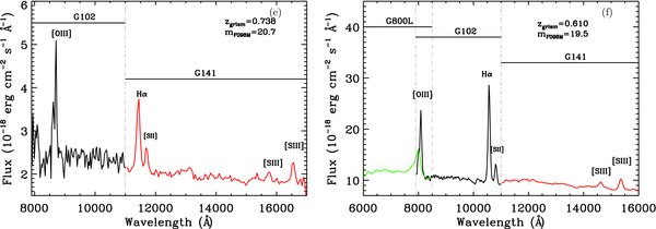
Figure 15. (a)–(d) 4212 s WFC3 G102 (top right) and G141 (bottom right) grism exposures of a single WFC3 pointing in the GOODS-South field (green box in Figure 3), together with their 1612 s finder images in F098M (top left) and G141 (bottom left), respectively. Each image is a 4-point dithered mosaic. (For best display, please zoom in on the full-resolution PDF version of this image.) All brighter object grism spectra show a zeroth-order image to their left, displaced by about twice the spectral image length, which should not be confused with real emission lines. Many faint object spectra are visible to a continuum flux of AB ≲ 25–25.5 mag, including many faint emission line galaxies. For details, see Straughn et al. (2009, 2011). (e) and (f) Examples of WFC3 G102 and G141 spectra of emission line galaxies extracted from the ERS grism images ((a)–(d)). The left panel shows an emission line galaxy at z = 0.738 and the right panel at z = 0.610. The latter also shows the available lower-resolution ACS G800L grism spectrum (green). The WFC3 G102 and G141 spectra allow for low-resolution faint object spectroscopy over the entire 0.80–1.70 μm range unimpeded by the ground-based OH-forest. For further details, see Straughn et al. (2009, 2011).
Download figure:
Standard image High-resolution image
Figures 15(e) and (f) show examples of some specific WFC3 G102 and G141 spectra for emission line galaxies in the ERS at z = 0.738 and z = 0.610. For the emission line galaxy at z = 0.610, the available lower-resolution ACS G800L grism spectrum is also shown in green. For further details, see Straughn et al. (2011). Figure 15(f) shows that WFC3 near-IR grisms G102 and G141 have a spectral resolution of R ≃ 210 and R≃ 130, respectively, while the ACS G800L has a lower resolution of R≃ 100. It is clear from Figure 15(f) that R ≳ 200 is far superior for faint emission-line (and by implication also for weak absorption feature) detection than an R ∼ 100 grism. This should be a critical consideration for the design of the JDEM/WFIRST missions that are now being planned (Blandford et al. 2010) to carry out wide-field near-infrared imaging and grism spectroscopy from space for this coming decade.
In conclusion, the WFC3 broadband IR filters and its G102 and G141 grisms provide low-resolution imaging and faint object spectroscopy over the entire 0.80–1.70 μm range, unimpeded by the ground-based OH forest. They have shown the tremendous power of the WFC3 IR grism data above Earth's atmosphere, which are now used by a number of different WFC3 GO programs in HST Cycle 17 and beyond. They also illustrate the discovery power of the new frontier that will be opened up by the near- to mid-infrared 6.5 m JWST after its launch in 2015 (Gardner et al. 2006; Windhorst et al. 2006), and by future wide-field near-infrared space missions such as JDEM/WFIRST and Euclid.
Footnotes
- *
Based on observations made with the NASA/ESA Hubble Space Telescope, which is operated by the Association of Universities for Research in Astronomy, Inc., under NASA contract NAS 5-26555.
- 25
- 26
- 27
- 28
- 29
- 30
- 31
- 32