


ABSTRACT
We report a spectral-line survey of the extreme carbon star IRC+10216 carried out between 293.9 and 354.8 GHz with the Submillimeter Array. A total of 442 lines were detected, more than 200 for the first time; 149 are unassigned. Maps at an angular resolution of ∼3'' were obtained for each line. A substantial new population of narrow lines with an expansion velocity of ∼4 km s−1 (i.e., ≈30% of the terminal velocity) was detected. Most of these are attributed to rotational transitions within vibrationally excited states, emitted from energy levels above the v = 0, J = 0 ground state with excitation energy of 1000–3000 K. Emission from these lines appears to be centered on the star with an angular extent of <1''. We use multiple transitions detected in several molecules to derive physical conditions in this inner envelope of IRC+10216.
Export citation and abstract BibTeX RIS
1. INTRODUCTION
Understanding the formation of complex molecules and dust grains in space is a major problem in modern astrophysics. Stars on the asymptotic giant branch (AGB) efficiently produce C, N, O, and s-process elements. Mass loss leads to the formation of expanding circumstellar envelopes (CSEs) whose molecules and dust grains are major sources of replenishment of the interstellar medium (Herwig 2005; Busso et al. 1999). The radius of the C/O core, after the exhaustion of core He burning, is Rc ≈ 109 cm, and the temperature is ∼108 K. He burning continues in a shell around the core and the size of the stellar photosphere expands to R* ≈ 1013 cm. During the phase of intermittent burning of H and He (in the so-called thermal pulse), products of nuclear burning are dredged up by convection and brought to the stellar surface. The zone within a few stellar radii is dynamically important for mass loss; in this zone molecules produced in the stellar atmosphere are moved to a region away from the star that is cool enough (∼1000 K) so that dust grains can condense. Radiation pressure on the grains drives the CSE's expansion. The outer circumstellar region is comparatively less dense by several orders of magnitude and richer in molecular gas, steadily expanding outward with velocities ∼10 km s−1. The chemistry in the outermost part of the circumstellar shell is driven by the interstellar UV radiation (Glassgold 1996). Due to the clumpy nature of the shell, photochemistry may be important in the inner regions as well (Decin et al. 2010).
IRC+10216 (CW Leo) is a well-known AGB carbon star ([C] > [O] and the presence of s-process elements) with a high mass-loss rate (several ×10−5 M☉ yr−1) at a distance of 150 pc (e.g., Young et al. 1993; Crosas & Menten 1997). Owing to its closeness to the Sun, it has been possible to study the physical and chemical processes in its large CSE in great detail (e.g., Olofsson 1999). There are nearly 60 molecules observed in the circumstellar shell of IRC+10216 as a result of previous single-dish line surveys (Kawaguchi et al. 1995; Cernicharo et al. 2000; Avery et al. 1992; Groesbeck et al. 1994; He et al. 2008; Ziurys et al. 2002; Cernicharo et al. 2010; Tenenbaum et al. 2010).
Mapping the spatial distribution of molecules in the CSE of IRC+10216 is important for several reasons: (1) molecular (and isotopic) abundances can be accurately determined, since the excitation temperature can be inferred from the spatial location of the molecules in the envelope; (2) such data can be readily and quantitatively compared with chemical models predicting abundances as a function of radial distance from the star; (3) parent molecules can be distinguished from product molecules given their distribution in the envelopes; (4) molecules important for the creation of dust can be identified (e.g., the distributions of SiO, SiS, SiN, and silicon carbides appear to be centrally concentrated near the region of dust formation and probably are dominant constituents of grains forming in this region, their abundance decreases with distance from the star); and (5) multiple transitions of the same molecule allow mapping of physical conditions (e.g., temperature) in the envelope.
Interferometric maps of NaCN, SiO, SiS, CS, HC5N, SiCC, NaCl, MgNC, CN, HNC, C2H, C3H, and C4H have been presented by Guélin et al. (1996) and Dayal & Bieging (1995). Except for the SiO J = 5–4 line at 217 GHz (Schöier et al. 2006) and the CS J = 14–13 line at 685 GHz (Young et al. 2004) mapped with the Submillimeter Array7 (SMA), all the other maps were obtained using the IRAM Plateau de Bure Interferometer (PdBI) or the Berkeley–Illinois–Maryland Array (BIMA) at around 100 GHz.
We selected the 345 GHz band for our survey primarily because very little data exist in this frequency range, and it contains transitions from many astrochemically important molecules, including various salts, the cyanopolyyne HC3N, and cyclic molecules such as C3H2. Two line surveys in the 345 GHz band have been published by Avery et al. (1992) in the frequency range of 339.6–364.6 GHz with a sensitivity of 0.3 K rms made with the 15 m diameter James Clerk-Maxwell Telescope (JCMT) and by Groesbeck et al. (1994), in the frequency range of 330.2–358.1 GHz, with the Caltech Submillimeter Observatory (CSO) 10.4 m telescope with an rms noise level of 65 mK (4.6 Jy). Our frequency range goes well beyond these surveys, including the range of 300–330 GHz, which is almost unexplored.
2. OBSERVATIONS AND DATA REDUCTION
The SMA observations of IRC+10216 were done in two periods, each about one week long. The first was 2007 January and February and the second 2009 February. All observations were made with the array in the subcompact configuration, with baselines from 9.5 m to 69.1 m. The typical synthesized beam size was 3'' × 2''. Table 1 summarizes the observational parameters for all observations. The duration of each track was from 7 to 9 hr. The phase center was at α(2000) = 09h47m57 38, δ(2000) = +13°16'43
 70 for all observations. All tracks in the first phase of observation (in 2007) were carried out in mosaiced mode, with five pointings with offsets in right ascension and declination of (0, ''0'') and (±12, '' ± 12''). The 2009 epoch observations were done with a single pointing toward IRC+10216. The u–v coverage and synthesized beam in one of the single-pointing tracks are shown in Figure 1. Titan and the quasars 0851+202 and 1055+018 were observed every 20 minutes for gain calibration. The spectral bandpass was calibrated by observations of Mars and Jupiter. Absolute flux calibration was determined by observations of Titan and Ganymede.

Figure 1. UV coverage and beam pattern. Emission extended over angular scales greater than 15'' is expected to get resolved out significantly.
Download figure:
Standard image High-resolution imageTable 1. Summary of Observations
| Date | LSB | USB | Synthesized | τ225 GHza | Tsysb |
|---|---|---|---|---|---|
| Coverage | Coverage | Beam | (SSB, K) | ||
| 2007 Jan 25 | 338.9–340.9 | 348.9–350.9 | 30 × 20, P.A. = −4° |
0.08 | 180–270 |
| 2007 Feb 5 | 338.4–340.1 | 348.7–350.0 | 30 × 20, P.A. = −4° |
0.08 | 180–270 |
| 2007 Feb 7 | 298.1–300.1 | 308.1–310.1 | 32 × 24, P.A. = −4° |
0.08 | 180–270 |
| 2007 Feb 8 | 300.1–302.1 | 310.1–312.1 | 33 × 24, P.A. = −6° |
0.09 | 160–230 |
| 2007 Feb 9 | 336.4–338.4 | 346.5–348.4 | 30 × 24, P.A. = −8° |
0.08 | 180–350 |
| 2007 Feb 10 | 334.5–336.4 | 344.5–346.4 | 30 × 24, P.A. = −8° |
0.08 | 180–350 |
| 2007 Feb 12 | 332.5–334.5 | 342.5–344.5 | 30 × 24, P.A. = −8° |
0.08 | 180–350 |
| 2009 Jan 22 | 302.0–306.0 | 313.9–317.9 | 33 × 23, P.A. = −24° |
0.05 | 100–200 |
| 2009 Jan 23 | 312.0–316.0 | 323.9–327.9 | 27 × 21, P.A. = −13° |
0.05 | 200–500 |
| 2009 Jan 26 | 315.9–319.9 | 327.9–331.9 | 27 × 21, P.A. = −13° |
0.08 | 200–400 |
| 2009 Jan 30 | 338.9–342.9 | 350.8–354.8 | 30 × 22, P.A. = −2° |
0.06 | 150–300 |
| 2009 Jan 31 | 319.9–323.9 | 331.9–335.8 | 30 × 24, P.A. = −6° |
0.08 | 280–700 |
| 2009 Feb 2 | 293.9–297.9 | 305.9–309.9 | 59 × 30, P.A. = 38° |
0.06 | 100–240 |
Notes. aZenith optical depth measured at 225 GHz with the CSO's radiometer. bTsys range is over all antennas and over the range of elevations covered during the observations of IRC+10216.
Download table as: ASCIITypeset image
The visibility data were calibrated with the Miriad package (Sault et al. 1995). For the 2007 data, the mosaiced images were de-convolved using the Miriad task mossdi; the resulting synthesized beams are summarized in Table 1. The single-pointing 2009 data were calibrated with the MIR-IDL package8 and imaged in Miriad using the standard tasks invert, clean, and restor. Maps of continuum emission show the peak to have a position offset of (Δα, Δδ) ≈ (07, 02) from the phase center position. The absolute position measurements for the continuum emission are estimated to be accurate to ∼01. Taking into account the proper motion of IRC+10216 of ( mas yr−1 determined by Menten et al. (2006), our position is consistent with theirs. The continuum emission was unresolved at the highest angular resolution of ∼08. The integrated continuum flux density was ∼650 mJy at 300 GHz and ∼1 Jy at 350 GHz, with an uncertainty of about 15% in the absolute flux calibration. The frequency resolution was 0.812 MHz per channel.
3. RESULTS
We detected a total of 442 lines. Of these, 297 could be assigned to known molecular transitions. Table 2 summarizes all detections, with fitted parameters and molecular assignments.
Table 2. Parameters of the Lines Detected in IRC+10216 in the SMA Line Survey
| No. | Species | Vib. State | Transition | νobs | σ | νcat | Δν | Vexp | σ | Peak | σ | Iint | θx | θy | P.A. |
|---|---|---|---|---|---|---|---|---|---|---|---|---|---|---|---|
| (MHz) | (MHz) | (MHz) | (MHz) | (km s−1) | (km s−1) | (Jy beam−1 km s−1) | (Jy) | (Jy km s−1) | ('') | ('') | (°) | ||||
| 1 | U | 293972.6 | 0.8 | 5.3 | 0.8 | 3.1 | 0.6 | 3.4 | ... | ... | ... | ||||
| 2 | CH3CN | 16(7)–15(7) | 294024.8 | 3.0 | 294024.8 | 0.0 | 14.2 | 4.8 | 4.0 | 0.2 | 4.7 | 2.4 | 0.7 | −2.2 | |
| 3 | U | 294056.3 | 0.8 | 2.1 | 0.8 | 3.1 | 0.1 | 3.1 | ... | ... | ... | ||||
| 4 | CH3CN | 16(6)–15(6) | 294099.7 | 2.5 | 294098.9 | 0.8 | 14.7 | 4.1 | 8.2 | 0.3 | 12.7 | 3.2 | 2.5 | −16.6 | |
| 5 | HCN | v2 + v3 | 36–36 | 294121.3 | 5.8 | 294121.3 | 0.0 | 5.4 | 3.9 | 2.1 | 0.3 | 1.7 | 0.0 | 0.0 | 0.0 |
| 6 | CH3CN | 16(5)–15(5) | 294162.1 | 2.7 | 294162.1 | 0.0 | 13.5 | 6.0 | 6.6 | 0.3 | 11.0 | 3.7 | 2.6 | −14.5 | |
| 7 | CH3CN | 16(4)–15(4) | 294213.0 | 1.6 | 294211.9 | 1.1 | 13.5 | 2.3 | 9.1 | 0.2 | 14.8 | 3.2 | 3.1 | −2.3 | |
| 8 | CH3CN | 16(3)–15(3) | 294252.8 | 0.5 | 294252.9 | −0.1 | 14.3 | 0.9 | 30.3 | 0.7 | 61.0 | 4.3 | 3.9 | 11.5 | |
| 9 | CH3CN | 16(0)–15(0) | 294299.2 | 0.6 | 294300.8 | −1.6 | 16.6 | 0.8 | 42.3 | 0.7 | 88.8 | 4.5 | 4.0 | 22.9 | |
| 10 | CH3CN | v8 = 1 | 16(13)–15(13) | 294383.7 | 1.3 | 294382.6 | 1.1 | 2.8 | 1.3 | 1.0 | 0.0 | 0.9 | 0.0 | 0.0 | 0.0 |
| 11 | 29Si34S | 17–16 | 294404.2 | 1.3 | 294403.3 | 0.9 | 14.1 | 1.3 | 7.0 | 0.2 | 10.5 | 3.0 | 2.5 | −9.1 | |
| 12 | CH3CN | v8 = 1 | 16(12)–15(12) | 294513.0 | 1.8 | 294512.9 | 0.1 | 4.3 | 0.3 | ... | ... | ... | ... | ... | ... |
| 13 | CH3CN | v8 = 1 | 16(11)–15(11) | 294630.1 | 1.0 | 294631.7 | −1.6 | 5.4 | 2.0 | 5.6 | 0.2 | 6.4 | 2.2 | 1.1 | 12.5 |
| 14 | NaCN ? | 19(9, 11)–18(9, 10) | 294671.3 | 3.4 | 294671.4 | −0.1 | 14.6 | 3.5 | 3.3 | 0.4 | 5.8 | 4.2 | 3.2 | 49.8 | |
| 15 | 30SiS | v = 2 | 17–16 | 294727.9 | 0.8 | 294727.1 | 0.8 | 2.3 | 0.1 | ... | ... | ... | ... | ... | ... |
| 16 | C4H | N = 31–30, J = 63/2–61/2 | 294915.8 | 1.0 | 294914.9 | 0.9 | ... | ... | ... | ... | ... | ... | ... | ... | |
| 17 | C4H | N = 31–30, J = 61/2–59/2 | 294953.3 | 0.4 | 294953.0 | 0.3 | ... | ... | ... | ... | ... | ... | ... | ... | |
| 18 | 29SiCC | 13(2, 12)–12(2, 11) | 295240.6 | 0.1 | 295237.5 | 3.1 | 13.9 | 0.1 | 11.6 | 0.6 | 24.7 | 4.6 | 4.0 | 72.6 | |
| 19 | U | 295401.2 | 0.3 | 4.0 | 0.2 | ... | ... | ... | ... | ... | ... | ||||
| 20 | U | 295450.1 | 0.3 | 4.9 | 0.4 | 1.4 | 0.1 | 1.6 | 2.5 | 0.8 | 24.7 | ||||
| 21 | U | 295519.3 | 0.4 | 4.1 | 0.4 | 1.1 | 0.2 | 1.9 | 3.8 | 2.1 | −62.5 | ||||
| 22 | U | 295542.6 | 0.5 | 4.4 | 0.1 | 0.7 | 0.0 | 0.6 | ... | ... | ... | ||||
| 23 | U | 295582.6 | 0.3 | 15.5 | 0.3 | 2.3 | 0.2 | 10.1 | 8.4 | 6.7 | 2.1 | ||||
| 24 | U | 295607.7 | 0.6 | 5.0 | 1.1 | 0.9 | 0.2 | 1.2 | 3.5 | 1.8 | 66.2 | ||||
| 25 | Si13CC | 13(11, 2)–12(11, 1) | 295699.9 | 0.4 | 295700.8 | −0.9 | 2.3 | 0.6 | 0.7 | 0.0 | 1.2 | 3.6 | 3.0 | 71.9 | |
| 26 | U | 295721.9 | 0.6 | 4.1 | 0.8 | 0.6 | 0.1 | 1.9 | 8.7 | 4.2 | 47.5 | ||||
| 27 | Si34S | v = 3 | 17–16 | 295753.6 | 0.1 | 295748.6 | 5.0 | 6.2 | 0.1 | 2.9 | 0.2 | 4.1 | 2.7 | 2.3 | −86.6 |
| 28 | U | 295772.0 | 1.4 | ... | ... | 5.1 | 0.3 | 10.9 | 4.6 | 4.0 | 7.4 | ||||
| 29 | NaCN ? | 19(7, 13)–18(7, 12) | 295792.0 | 1.4 | 295791.8 | 0.2 | ... | ... | 4.6 | 0.3 | 9.5 | 4.4 | 3.8 | −40.5 | |
| 30 | 30SiCC | 14(0, 14)–13(0, 13) | 295960.9 | 1.2 | 295965.6 | −4.7 | 14.3 | 1.1 | 5.9 | 0.3 | 13.0 | 4.8 | 4.0 | −73.9 | |
| 31 | 30SiS | v = 1 | 17–16 | 296150.9 | 2.1 | 296149.7 | 1.2 | 6.0 | 1.2 | 3.5 | 0.1 | 3.9 | 2.1 | 0.2 | 6.1 |
| 32 | NaCN | 19(6, 14)–18(6, 13) | 296340.7 | 4.0 | 296342.5 | −1.8 | 13.0 | 4.6 | 3.5 | 0.2 | 5.3 | 3.3 | 2.0 | −66.0 | |
| 33 | U | 296465.6 | 2.7 | 4.6 | 1.9 | 1.8 | 0.2 | 2.1 | 2.2 | 1.6 | 36.6 | ||||
| 34 | SiCC | v3 = 1 | 13(9, 4)–12(9, 3) | 296491.7 | 3.7 | 296489.9 | 1.8 | 9.4 | 6.8 | 8.4 | 0.3 | 10.1 | 2.1 | 1.6 | 3.0 |
| 35 | U | 296528.6 | 2.6 | 13.9 | 2.6 | 2.6 | 0.1 | 11.3 | 8.0 | 7.4 | 64.0 | ||||
| 36 | 30SiO | 7–6 | 296575.7 | 0.1 | 296575.7 | 0.0 | 13.9 | 0.1 | 91.8 | 2.1 | 165.6 | 3.9 | 3.5 | 31.6 | |
| 37 | SiCC | v3 = 1 | 14(1, 14)–13(1, 13) | 296658.6 | 2.8 | 296657.7 | 0.9 | 12.4 | 4.8 | 13.1 | 0.3 | 15.4 | 1.9 | 1.3 | −14.0 |
| 38 | AlF | 9–8 | 296699.0 | 0.3 | 296698.9 | 0.1 | 14.0 | 0.2 | 31.8 | 1.3 | 88.8 | 5.6 | 5.5 | 61.1 | |
| 39 | U | 296909.6 | 0.6 | 3.1 | 0.6 | 1.2 | 0.2 | 1.5 | 3.0 | 0.7 | 72.3 | ||||
| 40 | NaCN | 19(5, 14)–18(5, 13) | 296951.4 | 1.1 | 296955.1 | −3.7 | 11.2 | 1.2 | 3.3 | 0.2 | 5.4 | 3.6 | 2.1 | −57.6 | |
| 41 | 29SiS | v = 4 | 17–16 | 297007.7 | 2.3 | 297006.5 | 1.2 | 5.0 | 1.2 | 0.9 | 0.0 | 1.0 | 2.2 | 0.6 | 32.3 |
| 42 | 29Si33S | v = 1 | 17–16 | 297068.8 | 1.1 | 297063.4 | 5.4 | 12.3 | 1.2 | 1.3 | 0.1 | 1.9 | 3.3 | 2.0 | −43.9 |
| 43 | U | 297119.6 | 2.5 | 3.6 | 4.8 | ... | ... | ... | ... | ... | ... | ||||
| 44 | U | 297155.5 | 1.0 | 14.3 | 1.0 | 4.6 | 0.4 | 11.6 | 5.4 | 4.8 | 24.2 | ||||
| 45 | Si34S | v = 2 | 17–16 | 297190.7 | 1.0 | 297189.4 | 1.3 | 3.3 | 0.2 | 1.2 | 0.0 | 1.0 | ... | ... | ... |
| 46 | KCl | v = 1 | 39–38 | 297262.5 | 1.1 | 297261.8 | 0.8 | 11.1 | 1.1 | 1.3 | 0.2 | 4.2 | 7.1 | 4.9 | −29.0 |
| 47 | 13CCS ? | N = 31–30, J = 30–30 | 297467.4 | 2.4 | 297465.7 | 1.7 | 15.1 | 2.4 | 4.8 | 0.3 | 7.3 | 3.2 | 2.7 | 64.0 | |
| 48 | U | 297527.8 | 2.6 | 14.0 | 2.9 | 1.9 | 0.2 | 10.6 | 10.0 | 8.2 | −3.1 | ||||
| 49 | 30SiS | 17–16 | 297572.6 | 0.0 | 297572.2 | 0.4 | 13.8 | 0.0 | 124.9 | 3.1 | 217.4 | 3.7 | 3.3 | 21.5 | |
| 50 | U | 297602.2 | 2.0 | 7.8 | 2.3 | 3.9 | 0.1 | 5.5 | 2.8 | 2.2 | 3.2 | ||||
| 51 | NaCN | 19(4, 16)–18(4, 15) | 297630.9 | 5.1 | 297631.7 | −0.8 | 14.6 | 5.8 | 1.5 | 0.1 | 2.3 | 2.9 | 2.6 | −22.4 | |
| 52 | SiCC | 12(2, 10)–11(2, 9) | 297687.6 | 0.0 | 297687.7 | −0.1 | 14.5 | 0.1 | 156.3 | 5.0 | 456.3 | 5.9 | 5.6 | 47.1 | |
| 53 | Si34S | v = 1 | 17–16 | 298630.4 | 0.7 | 298630.0 | 0.4 | 4.4 | 4.0 | 1.88 | 0.1 | 2.17 | 1.16 | 0.98 | −9 |
| 54 | Al37Cl | 21–20 | 298670.9 | 0.2 | 298670.8 | 0.1 | 13.8 | 0.2 | 9.85 | 0.623 | 17.7 | 2.81 | 2.02 | −48 | |
| 55 | KCl | 39–38 | 299103.7 | 0.3 | 299100.9 | 2.8 | 9.6 | 1.2 | 5.05 | 0.633 | 5.58 | ... | ... | ... | |
| 56 | NaCl | 23–22 | 299145.1 | 0.3 | 299145.7 | −0.6 | 12.3 | 0.5 | 13.3 | 0.857 | 18.9 | 2.07 | 1.55 | −18 | |
| 57 | SiCC | 13(2, 12)–12(2, 11) | 299277.4 | 0.0 | 299277.0 | 0.4 | 14.2 | 0.0 | 94.8 | 2.70 | 229 | 3.30 | 3.16 | 85 | |
| 58 | SiCC | v3 = 2 | 13(4, 9)–12(4, 8) | 299403.0 | 0.2 | 299400.2 | 2.8 | 7.2 | 5.9 | 1.68 | 0.259 | 3.65 | 4.96 | 1.47 | −10 |
| 59 | SiS | v = 6 | 17–16 | 299503.2 | 0.1 | 299502.2 | 1.0 | 3.1 | 2.0 | 0.533 | 0.122 | 3.38 | 8.54 | 4.66 | −20 |
| 60 | 29SiCC | 14(0, 14)–13(0, 13) | 299546.6 | 0.2 | 299546.5 | 0.1 | 14.7 | 1.1 | 1.44 | 0.253 | 9.29 | 7.18 | 5.70 | 33 | |
| 61 | 29SiO | 7–6 | 300120.4 | 0.1 | 300121.1 | −0.7 | 14.1 | 0.2 | 78.5 | 1.26 | 162 | 2.99 | 2.73 | 47 | |
| 62 | HC3N | 33–32 | 300159.9 | 0.6 | 300159.7 | 0.2 | 14.4 | 0.2 | 11.7 | 0.415 | 29.2 | 3.79 | 3.08 | −10 | |
| 63 | HC3N | v5 + 3v7 | 33–32 | 300348.3 | 1.8 | 300347.3 | 1.0 | 4.3 | 6.7 | 2.58 | 0.430 | 4.61 | 3.53 | 1.42 | −40 |
| 64 | U | 300619.0 | 0.1 | 5.3 | 4.5 | ... | ... | ... | ... | ... | ... | ||||
| 65 | 29SiCC | 13(8, 6)–12(8, 5) | 300756.5 | 0.4 | 300750.8 | 5.7 | 7.5 | 4.1 | 3.10 | 0.707 | 9.59 | 5.45 | 2.50 | −75 | |
| 66 | 29SiS | v = 1 | 17–16 | 301390.4 | 0.3 | 301388.9 | 1.5 | 4.8 | 3.2 | 3.49 | 0.447 | 4.84 | 2.59 | 0.98 | −19 |
| 67 | SiCC | 13(12, 1)–12(12, 0) | 301550.1 | 0.3 | 301549.9 | 0.2 | 15.3 | 7.2 | 3.09 | 0.232 | 5.69 | 3.29 | 1.96 | −2 | |
| 68 | SiO | v = 1 | 7–6 | 301816.7 | 0.4 | 301814.3 | 2.4 | 9.5 | 3.4 | 4.96 | 0.685 | 7.68 | 2.70 | 1.48 | −28 |
| 69 | U | 302069.7 | 1.1 | 6.1 | 1.3 | ... | ... | ... | ... | ... | ... | ||||
| 70 | HC3N | v5 + v6 + v7 | 33–32 | 302118.6 | 1.4 | 302120.6 | −2.0 | 14.3 | 1.1 | ... | ... | ... | ... | ... | ... |
| l = −1, 1, 1 | - | ||||||||||||||
| 71 | SiCC | v3 = 1 | 13(5, 9)–12(5, 8) | 302184.5 | 0.7 | 302182.3 | 2.2 | 7.5 | 0.0 | 6.2 | 1.3 | 9.3 | ... | ... | ... |
| 72 | SiCC | v3 = 1 | 13(5, 8)–12(5, 7) | 302238.6 | 0.9 | 302237.7 | 0.9 | 11.1 | 0.9 | 7.3 | 0.8 | 8.7 | ... | ... | ... |
| 73 | U | 302531.5 | 0.7 | 3.8 | 0.8 | 2.5 | 0.6 | 2.6 | ... | ... | ... | ||||
| 74 | SiCC | v3 = 1 | 13(1, 12)–12(1, 11) | 302583.2 | 1.1 | 302579.0 | 4.2 | 9.1 | 0.1 | 9.5 | 2.2 | 21.0 | 5.6 | 2.5 | −54.6 |
| 75 | HC3N | v5 + v6 + 2v7 | 33–32 | 302696.4 | 1.9 | 302694.8 | 1.6 | 10.4 | 2.7 | 1.7 | 0.1 | 1.7 | ... | ... | ... |
| l = −1, 1, 2 | |||||||||||||||
| 76 | HC3N | v5 + v6 + 2v7 | 33–32 | 302763.0 | 0.5 | 302768.7 | −5.7 | 4.0 | 0.5 | ... | ... | ... | ... | ... | ... |
| l = 1, 1, − 2 | |||||||||||||||
| 77 | 29SiS | 17–16 | 302850.8 | 0.3 | 302849.5 | 1.3 | 14.0 | 0.1 | 266.4 | 10.4 | 439.9 | 3.7 | 2.6 | −24.6 | |
| 78 | CH3C15N | 17(5)–16(5) | 303137.0 | 2.4 | 303136.4 | 0.6 | 7.0 | 2.4 | ... | ... | ... | ... | ... | ... | |
| 79 | SiCC | 14(0, 14)–13(0, 13) | 303373.9 | 0.1 | 303373.2 | 0.7 | 14.0 | 0.1 | ... | ... | ... | ... | ... | ... | |
| 80 | SiCC | 13(10, 3)–12(10, 2) | 303441.0 | 0.8 | 303440.3 | 0.7 | 14.3 | 0.8 | 51.8 | 4.6 | 81.0 | 3.6 | 1.6 | −33.8 | |
| 81 | U | 303512.7 | 0.2 | 4.3 | 0.2 | ... | ... | ... | ... | ... | ... | ||||
| 82 | U | 303842.9 | 0.6 | 12.7 | 0.6 | ... | ... | ... | ... | ... | ... | ||||
| 83 | SiO | 7–6 | 303927.7 | 0.0 | 303926.8 | 0.9 | 13.5 | 0.1 | ... | ... | ... | ... | ... | ... | |
| 84 | U | 303980.9 | 1.7 | 5.8 | ... | ... | ... | ... | ... | ... | |||||
| 85 | SiS | v = 3 | 17–16 | 304008.4 | 0.7 | 304010.3 | −1.9 | 7.6 | 2.7 | 8.3 | 1.3 | 8.6 | |||
| 86 | Si33S | 17–16 | 304160.0 | 0.1 | 304159.2 | 0.8 | 14.2 | 0.1 | 32.1 | 1.0 | 67.1 | 3.0 | 2.9 | 77.3 | |
| 87 | U | 304189.3 | 0.8 | 3.3 | 1.5 | 1.7 | 0.3 | 2.9 | 3.8 | 1.4 | −37.5 | ||||
| 88 | U | 304247.7 | 0.7 | 5.0 | 1.3 | 3.5 | 0.5 | 4.5 | 2.4 | 1.0 | −27.9 | ||||
| 89 | U | 304279.8 | 1.0 | 3.1 | 1.1 | 1.3 | 0.3 | 3.1 | 4.4 | 1.9 | 36.9 | ||||
| 90 | HC3N | 2v6 + 3v7 | 33–32 | 304308.0 | 2.0 | 304307.1 | 0.9 | 13.3 | 2.2 | ... | ... | ... | ... | ... | ... |
| l = 0, 2, 3f | |||||||||||||||
| 91 | C4H | N = 32–31 | 304423.8 | 2.0 | 304422.0 | 1.8 | 13.8 | 1.0 | ... | ... | ... | ... | ... | ... | |
| J = 65/2–63/2 | |||||||||||||||
| 92 | C4H | N = 32–31 | 304460.0 | 1.0 | 304459.9 | 0.1 | 14.7 | 1.0 | ... | ... | ... | ... | ... | ... | |
| J = 63/2–61/2 | |||||||||||||||
| 93 | U | 304547.2 | 2.1 | 19.9 | 2.0 | ... | ... | ... | ... | ... | ... | ||||
| 94 | HC3N | v5 + 4v7 | 33–32 | 304603.7 | 0.7 | 8.3 | 2.6 | ... | ... | ... | ... | ... | ... | ||
| l = 1, 0, 0e | |||||||||||||||
| 95 | 29SiCC | 13(4, 10)–12(4, 9) | 304683.0 | 0.2 | 304681.8 | 1.2 | 14.6 | 1.6 | ... | ... | ... | ... | ... | ... | |
| 96 | U | 304770.0 | 0.2 | 11.9 | 0.0 | ... | ... | ... | ... | ... | ... | ||||
| 97 | U | 305134.9 | 0.6 | 4.8 | 1.3 | 2.4 | 0.2 | 4.2 | 3.8 | 1.5 | −27.6 | ||||
| 98 | SiCC | 13(8, 5)–12(8, 4) | 305197.5 | 0.1 | 305196.7 | 0.8 | 14.6 | 0.1 | 71.1 | 2.9 | 196.9 | 4.0 | 3.6 | 34.4 | |
| 99 | SiN | N = 7–6 | 305286.9 | 0.0 | 305286.9 | 0.0 | ... | ... | ... | ... | ... | ... | ... | ... | |
| J = 13/2–11/2 | |||||||||||||||
| 100 | K37Cl | 41–40 | 305445.2 | 1.6 | 305442.3 | 2.9 | 14.1 | 7.0 | 11.9 | 0.7 | 16.7 | 1.8 | 1.8 | −72.5 | |
| 101 | SiS | v = 2 | 17–16 | 305513.7 | 0.9 | 305512.4 | 1.3 | 6.6 | 1.8 | 13.1 | 0.7 | 13.6 | 0.7 | 0.4 | −76.8 |
| 102 | U | 305578.7 | 1.6 | 4.8 | 3.2 | 2.3 | 0.3 | 3.1 | 2.0 | 1.3 | 7.9 | ||||
| 103 | 29SiCC | 13(4, 9)–12(4, 8) | 305702.1 | 1.2 | 305700.9 | 1.2 | 14.2 | 0.4 | 8.5 | 0.6 | 18.7 | 3.3 | 2.9 | −83.1 | |
| 104 | SiN | N = 7–6 | 305792.2 | 0.0 | 305792.2 | 0.0 | ... | ... | ... | ... | ... | ... | ... | ... | |
| J = 15/2–13/2 | |||||||||||||||
| 105 | AlCl | 21–20 | 305849.8 | 0.2 | 305850.6 | −0.8 | 14.0 | 0.4 | 45.8 | 1.6 | 93.0 | 3.0 | 2.8 | 39.0 | |
| 106 | 30Si34S | 18–17 | 306120.0 | 0.4 | 306119.9 | 0.1 | 15.5 | 0.2 | 8.6 | 0.3 | 13.3 | 3.2 | 2.6 | 49.6 | |
| 107 | CH2NH | 5(1, 5)–4(1, 4) | 306172.6 | 0.2 | 306172.2 | 0.4 | 14.1 | 0.2 | 4.0 | 0.2 | 15.5 | 7.2 | 6.3 | 80.1 | |
| 108 | U | 306226.7 | 0.3 | 3.2 | 0.2 | 2.1 | 0.1 | 2.9 | 2.4 | 2.1 | −84.1 | ||||
| 109 | U | 306282.4 | 0.6 | 3.6 | 0.6 | 1.0 | 0.1 | 1.3 | 2.8 | 1.1 | −4.4 | ||||
| 110 | U | 306316.5 | 0.6 | 7.3 | 0.8 | 2.4 | 0.3 | 3.1 | 2.0 | 1.8 | −51.9 | ||||
| 111 | U | 306449.4 | 0.5 | 4.2 | 0.7 | 1.2 | 0.1 | 1.4 | 2.3 | 1.5 | 36.0 | ||||
| 112 | SiCC | 16(2, 15)–16(0, 16) | 306485.7 | 0.3 | 306487.5 | −1.8 | 16.0 | 0.3 | 2.7 | 0.2 | 5.7 | 4.9 | 3.4 | 6.4 | |
| 113 | U | 306698.0 | 0.9 | 4.2 | 1.3 | 0.8 | 0.1 | 0.8 | ... | ... | ... | ||||
| 114 | KCl | 40–39 | 306729.5 | 0.4 | 306728.9 | 0.6 | 13.8 | 0.4 | 7.6 | 0.4 | 9.2 | 1.9 | 0.8 | −59.2 | |
| 115 | U | 306924.6 | 0.1 | 10.2 | 0.1 | 1.9 | 0.3 | 3.1 | 4.2 | 1.9 | 7.2 | ||||
| 116 | SiCC | 13(6, 7)–12(6, 6) | 307008.9 | 0.0 | 307009.3 | −0.4 | 14.4 | 0.0 | 206.9 | 7.5 | 448.1 | 4.5 | 4.0 | 28.9 | |
| 117 | SiCC | 20(2, 18)–20(2, 19) | 307056.8 | 0.7 | 307058.0 | −1.2 | 13.7 | 0.8 | 1.7 | 0.1 | 4.0 | 5.5 | 4.0 | 24.2 | |
| 118 | U | 307147.4 | 0.7 | 4.7 | 0.1 | 1.2 | 0.0 | 1.3 | 2.9 | 0.4 | 54.5 | ||||
| 119 | H3O+ | 1(1, 1)–2(1, 2) | 307199.5 | 0.3 | 307192.4 | 7.1 | 4.4 | 0.0 | 1.8 | 0.1 | 2.0 | ... | ... | ... | |
| 120 | U | 307304.7 | 0.3 | 13.8 | 0.3 | 1.3 | 0.2 | 12.7 | 14.0 | 10.4 | 32.0 | ||||
| 121 | U | 307471.0 | 0.5 | 4.2 | 0.6 | 1.2 | 0.1 | 1.2 | ... | ... | ... | ||||
| 122 | U | 307520.6 | 0.2 | 6.7 | 0.2 | 4.3 | 0.3 | 4.5 | 0.9 | 0.7 | −77.7 | ||||
| 123 | U | 307693.4 | 0.2 | 18.1 | 0.1 | 1.6 | 0.4 | 5.0 | 6.1 | 5.1 | −49.0 | ||||
| 124 | U | 307735.5 | 0.2 | 2.9 | 0.4 | 0.8 | 0.2 | 0.7 | ... | ... | ... | ||||
| 125 | U | 308024.5 | 0.2 | 2.5 | 0.2 | 0.8 | 0.0 | 0.8 | ... | ... | ... | ||||
| 126 | U | 308038.0 | 0.2 | 2.7 | 0.2 | 1.3 | 0.1 | 1.4 | 2.9 | 0.5 | 37.3 | ||||
| 127 | U | 308217.6 | 0.2 | 8.4 | 0.1 | 3.4 | 0.2 | 4.0 | 2.1 | 1.3 | 13.3 | ||||
| 128 | U | 308337.1 | 1.7 | 3.9 | 0.5 | 0.4 | 0.1 | 2.2 | 15.5 | 3.4 | −64.0 | ||||
| 129 | NaCN | 21(0, 21)–20(1, 20) | 308368.6 | 0.2 | 308373.4 | −4.8 | 3.4 | 0.2 | 1.0 | 0.2 | 1.8 | 3.4 | 3.1 | −10.5 | |
| 130 | SiS | 17–16 | 308517.5 | 0.0 | 308516.1 | 1.4 | 14.6 | 0.0 | 1605.0 | 37.4 | 3714.0 | 4.6 | 4.3 | 23.0 | |
| 131 | U | 309201.4 | 3.2 | 3.2 | 2.7 | 0.9 | 0.1 | 1.0 | ... | ... | ... | ||||
| 132 | U | 309223.4 | 3.0 | 6.0 | 0.7 | 4.6 | 0.3 | 5.0 | ... | ... | ... | ||||
| 133 | HC3N | 34–33 | 309251.7 | 0.5 | 309250.4 | 1.3 | 13.9 | 0.5 | 23.5 | 0.6 | 50.3 | 4.4 | 3.9 | 6.2 | |
| 134 | SiCC | 13(4, 10)–12(4, 9) | 309287.2 | 0.0 | 309286.5 | 0.7 | 14.2 | 0.0 | 137.0 | 5.3 | 343.8 | 5.0 | 4.6 | 35.6 | |
| 135 | U | 309360.6 | 3.7 | 6.8 | 0.6 | 4.2 | 0.2 | 4.7 | ... | ... | ... | ||||
| 136 | U | 309726.8 | 0.1 | 15.5 | 0.1 | 2.6 | 0.2 | 5.3 | 4.3 | 3.7 | 19.9 | ||||
| 137 | HCC13CN | 34–33 | 309793.2 | 0.4 | 309790.7 | 2.5 | 4.7 | 0.6 | 2.0 | 0.1 | 2.3 | ... | ... | ... | |
| 138 | SiCC | v3 = 2 | 14(2, 13)–13(2, 12) | 309849.2 | 0.2 | 309846.2 | 3.0 | 7.9 | 0.3 | 5.6 | 0.3 | 6.5 | 2.2 | 1.1 | 56.5 |
| 139 | U | 310368.3 | 7.3 | 10.7 | 0.1 | ... | ... | ... | ... | ... | ... | ||||
| 140 | SiCC | 13(4,9)–12(4,8) | 310439.0 | 0.0 | 310438.8 | 0.2 | 14.2 | 0.0 | 88.4 | 2.86 | 204 | 3.17 | 2.93 | 68 | |
| 141 | HCN | v2 = 1 | 37–37 | 310472.6 | 6.8 | 310471.8 | 0.8 | 3.6 | 0.3 | 0.932 | 1.4E-02 | 1.11 | 1.49 | 0.92 | −4 |
| 142 | KCN ? | 33(8, 26)–32(8, 25) | 310543.7 | 7.4 | 310544.2 | −0.5 | 2.2 | 0.5 | 0.854 | 7.4E-02 | 1.52 | 3.90 | 1.18 | −3 | |
| 143 | U | 310548.7 | 5.3 | 2.4 | 0.7 | 0.787 | 0.177 | 4.07 | 9.06 | 3.12 | 15 | ||||
| 144 | SiCC | v3 = 2 | 15(0, 15)–14(0, 14) | 310930.3 | 0.9 | 310931.0 | −0.7 | 9.4 | 0.2 | 2.73 | 0.267 | 3.70 | 1.98 | 1.25 | 22 |
| 145 | NaCN ? | 20(7, 14)–19(7, 13) | 311362.6 | 0.4 | 311363.2 | −0.6 | 13.2 | 0.5 | 1.20 | 9.5E-02 | 2.68 | 5.18 | 0.64 | −47 | |
| 146 | 29Si34S | 18–17 | 311708.0 | 0.1 | 311707.6 | 0.4 | 14.0 | 0.6 | 1.30 | 0.197 | 16.1 | 9.92 | 8.27 | 68 | |
| 147 | U | 311960.8 | 1.3 | 12.9 | 0.2 | ... | ... | ... | ... | ... | ... | ||||
| 148 | U | 312042.3 | 1.0 | 9.3 | 0.9 | 4.3 | 0.2 | 6.1 | 4.4 | 1.5 | 41.7 | ||||
| 149 | NaCl | 24–23 | 312109.9 | 0.3 | 312109.9 | 0.0 | 13.0 | 0.8 | 21.7 | 0.9 | 28.0 | 2.0 | 1.8 | 68.7 | |
| 150 | U | 312165.7 | 1.5 | 6.2 | 0.4 | 3.2 | 0.5 | 5.7 | 5.1 | 1.5 | 64.4 | ||||
| 151 | SiCC | v3 = 1 | 13(3, 10)–12(3, 9) | 312341.7 | 0.3 | 312338.8 | 2.9 | 10.8 | 0.4 | 6.6 | 0.8 | 9.4 | 2.6 | 2.0 | 4.5 |
| 152 | H2C4 | 35(0, 35)–34(0, 34) | 312419.4 | 1.1 | 312418.5 | 0.9 | 10.6 | 5.5 | 2.1 | 0.4 | 3.5 | 6.0 | 1.7 | 30.6 | |
| 153 | CH3CN | 17(6)–16(6) | 312472.7 | 0.5 | 312472.6 | 0.1 | 14.6 | 1.2 | 9.6 | 0.7 | 16.0 | 3.8 | 2.5 | 39.0 | |
| 154 | U | 312541.7 | 0.8 | 14.2 | 1.6 | 5.4 | 0.5 | 16.3 | 5.7 | 4.6 | −80.5 | ||||
| 155 | CH3CN | 17(3)–16(3) | 312634.3 | 0.2 | 312633.7 | 0.6 | 13.2 | 0.2 | 25.1 | 1.3 | 49.2 | 4.0 | 3.3 | 32.7 | |
| 156 | CH3CN | 17(1)–16(1) | 312684.2 | 0.2 | 312683.3 | 0.9 | 17.1 | 0.2 | 38.4 | 1.6 | 83.9 | 4.7 | 3.6 | 23.8 | |
| 157 | SiCC | v3 = 2 | 13(2, 11)–12(2, 10) | 312728.8 | 0.4 | 312730.1 | −1.3 | 3.5 | 0.5 | 4.1 | 0.1 | 4.2 | ... | ... | ... |
| 158 | 30SiCC | 14(2, 13)–13(2, 12) | 312817.3 | 1.0 | 312815.7 | 1.6 | 15.2 | 1.4 | 3.4 | 0.4 | 13.5 | 8.4 | 5.3 | 38.5 | |
| 159 | Al37Cl | 22–21 | 312867.0 | 0.3 | 312865.0 | 2.0 | 14.4 | 0.3 | 24.2 | 1.8 | 38.3 | 3.3 | 2.5 | 38.0 | |
| 160 | H2C4 | 35(2, 33)–34(2, 32) | 313570.5 | 0.9 | 313572.2 | −1.7 | 13.9 | 1.0 | 5.4 | 0.4 | 5.3 | ... | ... | ... | |
| 161 | H2C4 | 35(1, 34)–34(1, 33) | 313788.1 | 0.5 | 313792.3 | −4.2 | 6.5 | 0.5 | 3.1 | 0.1 | 3.2 | ... | ... | ... | |
| 162 | U | 314075.6 | 0.4 | 5.5 | 0.6 | 3.2 | 0.2 | 3.4 | 0.8 | 0.6 | 53.3 | ||||
| 163 | U | 314174.6 | 0.3 | 4.0 | 0.4 | 3.4 | 0.3 | 3.9 | 1.1 | 0.8 | −34.8 | ||||
| 164 | U | 314228.9 | 0.3 | 7.0 | 0.1 | 3.8 | 0.4 | 4.0 | ... | ... | ... | ||||
| 165 | U | 314270.8 | 0.2 | 3.8 | 1.0 | 0.9 | 0.2 | 1.2 | 2.3 | 1.2 | −28.2 | ||||
| 166 | KCN ? | 34(17, 18)–33(17, 17) | 314290.1 | 0.7 | 314289.5 | 0.6 | 4.6 | 0.5 | ... | ... | ... | ... | ... | ... | |
| 167 | KCl | 41–40 | 314354.8 | 0.5 | 314353.8 | 1.0 | 13.6 | 0.5 | 9.1 | 0.5 | 11.2 | 1.7 | 1.0 | −41.9 | |
| 168 | 29SiS | v = 4 | 18–17 | 314463.6 | 0.4 | 314462.9 | 0.7 | 4.8 | 0.3 | 0.6 | 0.0 | 0.9 | ... | ... | ... |
| 169 | U | 314540.8 | 0.2 | 3.2 | 0.1 | 0.7 | 0.0 | 0.7 | ... | ... | ... | ||||
| 170 | U | 314600.9 | 0.4 | 3.6 | 0.3 | 1.2 | 0.0 | 1.1 | ... | ... | ... | ||||
| 171 | U | 314630.1 | 0.5 | 3.3 | 0.6 | 0.7 | 0.0 | 0.7 | ... | ... | ... | ||||
| 172 | Si34S | v = 2 | 18–17 | 314659.0 | 0.2 | 314656.9 | 2.1 | 5.3 | 0.2 | 2.7 | 0.3 | 2.9 | 0.8 | 0.5 | 78.9 |
| 173 | Si13CC | 13(2, 11)–12(2, 10) | 314814.4 | 0.2 | 314814.1 | 0.3 | 14.5 | 0.2 | 2.3 | 0.2 | 10.7 | 6.1 | 4.1 | 59.7 | |
| 174 | 30SiS | 18–17 | 315062.3 | 0.0 | 315062.5 | −0.2 | 14.3 | 0.0 | 110.0 | 3.4 | 220.2 | 2.7 | 2.7 | −44.0 | |
| 175 | SiC | 8–7,Ω = 2 | 315119.9 | 2.1 | 315119.9 | 0.0 | |||||||||
| 176 | NaCN | 20(1, 19)–19(1, 18) | 315215.4 | 4.0 | 315213.6 | 1.8 | 11.6 | 5.5 | 2.7 | 0.3 | 5.7 | 3.0 | 2.7 | −50.6 | |
| 177 | U | 315294.5 | 0.1 | 4.3 | 0.1 | 5.1 | 0.1 | 5.0 | ... | ... | ... | ||||
| 178 | U | 315317.3 | 0.2 | 3.4 | 0.3 | 2.6 | 0.2 | 2.7 | ... | ... | ... | ||||
| 179 | U | 315335.6 | 0.4 | 3.9 | 0.6 | 1.9 | 0.1 | 1.8 | ... | ... | ... | ||||
| 180 | U | 315428.3 | 0.3 | 6.2 | 0.1 | 3.4 | 0.3 | 3.3 | ... | ... | ... | ||||
| 181 | Si13CC | 15(1, 15)–14(1, 14) | 315635.2 | 0.2 | 315635.6 | −0.4 | 14.0 | 0.2 | 2.3 | 0.3 | 5.9 | 4.0 | 2.9 | −48.9 | |
| 182 | SiCC | v3 = 1 | 14(11, 3)–13(11, 2) | 316050.8 | 0.4 | 316048.5 | 2.3 | 4.0 | 0.6 | 6.6 | 0.3 | 10.5 | ... | ... | ... |
| 183 | Si34S | v = 1 | 18–17 | 316183.7 | 0.4 | 316184.6 | −0.9 | 9.1 | 0.5 | 14.7 | 1.4 | 23.1 | 3.1 | 2.4 | −28.4 |
| 184 | 13CS | v = 3 | 7–6 | 316842.7 | 0.6 | 316846.3 | −3.6 | 14.1 | 0.7 | 4.6 | 0.5 | 24.4 | 13.6 | 5.2 | 52.2 |
| 185 | U | 317094.5 | 0.7 | 3.2 | 0.4 | 1.2 | 0.1 | 1.6 | 2.6 | 0.7 | −69.8 | ||||
| 186 | SiCC | v3 = 1 | 15(1, 15)–14(1, 14) | 317153.6 | 0.4 | 317151.7 | 1.9 | 11.0 | 0.1 | 11.0 | 1.4 | 11.2 | ... | ... | ... |
| 187 | 29SiCC | 13(2, 11)–12(2, 10) | 317353.1 | 2.8 | 317350.7 | 2.4 | 14.1 | 2.0 | ... | ... | ... | ... | ... | ... | |
| 188 | U | 317395.1 | 0.4 | 3.5 | 0.4 | ... | ... | ... | ... | ... | ... | ||||
| 189 | U | 317419.6 | 0.4 | 1.5 | 2.2 | ... | ... | ... | ... | ... | ... | ||||
| 190 | 29SiS | v = 2 | 18–17 | 317558.3 | 0.3 | 317558.2 | 0.1 | 6.1 | 0.4 | 5.2 | 0.7 | 5.4 | |||
| 191 | Si34S | 18–17 | 317708.7 | 0.0 | 317707.4 | 1.3 | 14.0 | 0.0 | 191.3 | 7.9 | 313.3 | 3.4 | 1.8 | −37.0 | |
| 192 | HC3N | v4 | 35–34 | 317900.6 | 0.6 | 317894.3 | 6.3 | 3.5 | 1.5 | ... | ... | ... | ... | ... | ... |
| 193 | U | 317935.8 | 1.0 | 7.5 | 0.2 | ... | ... | ... | ... | ... | ... | ||||
| 194 | U | 318027.0 | 0.9 | 4.4 | 0.3 | 0.6 | 0.2 | 2.9 | 8.3 | 2.0 | −74.4 | ||||
| 195 | Na37Cl | 25–24 | 318127.5 | 0.4 | 318127.7 | −0.2 | 12.3 | 0.2 | 6.4 | 0.6 | 9.6 | 2.1 | 1.6 | −27.8 | |
| 196 | 13C34S | 7–6 | 318197.8 | 0.2 | 318197.5 | 0.3 | 13.6 | 0.4 | 6.0 | 0.4 | 11.1 | 2.6 | 2.2 | −44.8 | |
| 197 | U | 318286.7 | 1.1 | 19.7 | 2.2 | 5.3 | 0.7 | 10.6 | 3.6 | 1.7 | −25.8 | ||||
| 198 | HC3N | 35–34 | 318340.5 | 0.1 | 318340.8 | −0.3 | 13.7 | 0.2 | 13.0 | 0.7 | 41.5 | 4.2 | 3.5 | −4.9 | |
| 199 | U | 318412.5 | 0.7 | 4.1 | 0.5 | 2.0 | 0.6 | 7.0 | 6.6 | 1.9 | 53.1 | ||||
| 200 | 30SiCC | 21(2, 19)–21(2, 20) | 318442.8 | 0.2 | 318444.3 | −1.5 | 5.3 | 0.1 | 1.3 | 0.3 | 3.3 | 5.8 | 1.3 | 19.2 | |
| 201 | c-C3H2 | 8(2, 7)–7(1, 6) | 318483.3 | 0.5 | 318482.3 | 1.0 | 13.9 | 0.3 | 1.6 | 0.2 | 6.9 | 5.7 | 4.0 | −9.2 | |
| 202 | U | 318529.9 | 1.3 | 4.8 | 1.7 | 0.6 | 0.0 | 0.8 | ... | ... | ... | ||||
| 203 | U | 318566.8 | 0.4 | 2.2 | 1.0 | 0.8 | 0.0 | 1.0 | ... | ... | ... | ||||
| 204 | U | 318685.8 | 0.3 | 12.6 | 0.8 | 2.0 | 0.4 | 11.2 | 6.6 | 4.4 | −84.2 | ||||
| 205 | NaCN ? | 21(17, 4)–20(17, 3) | 318918.8 | 0.6 | 318922.3 | −3.5 | 3.1 | 0.3 | 1.6 | 0.1 | 1.6 | ... | ... | ... | |
| 206 | U | 318951.5 | 0.7 | 3.2 | 0.7 | 1.7 | 0.1 | 1.6 | ... | ... | ... | ||||
| 207 | U | 319021.1 | 0.8 | 13.6 | 2.0 | ... | ... | ... | ... | ... | ... | ||||
| 208 | HC3N | 35–34 | 319106.4 | 0.2 | 319112.2 | −5.8 | 8.3 | 0.5 | 3.9 | 0.2 | 4.1 | 0.8 | 0.2 | −58.2 | |
| 209 | SiCC | v3 = 1 | 14(9, 5)–13(9, 4) | 319382.6 | 0.4 | 319381.8 | 0.8 | 8.3 | 0.5 | 7.2 | 0.4 | 8.4 | 1.4 | 0.8 | −5.0 |
| 210 | HCP | 8–7 | 319571.8 | 0.2 | 319572.7 | −0.9 | 15.0 | 0.1 | 8.1 | 1.0 | 24.0 | 4.5 | 2.8 | −46.5 | |
| 211 | U | 319882.6 | 0.5 | 13.1 | 0.5 | 2.5 | 0.4 | 14.5 | 6.7 | 4.8 | −2.5 | ||||
| 212 | 29SiCC | 15(0, 15)–14(0, 14) | 320028.3 | 0.5 | 320027.1 | 1.2 | 13.7 | 0.5 | 7.0 | 0.9 | 19.3 | 5.2 | 3.9 | −45.3 | |
| 213 | NaCN | 21(16, 5)–20(16, 4) | 320133.2 | 1.1 | 320164.6 | −31.4 | 3.7 | 1.8 | 2.3 | 0.1 | 2.7 | ||||
| 214 | K37Cl | 43–42 | 320252.9 | 1.5 | 320253.0 | −0.1 | 7.2 | 1.4 | 1.9 | 0.2 | 3.5 | 3.9 | 2.8 | 46.9 | |
| 215 | SiS | v = 4 | 18–17 | 320288.0 | 0.8 | 320287.4 | 0.6 | 2.3 | 0.8 | 1.6 | 0.2 | 2.5 | 4.4 | 1.6 | 44.3 |
| 216 | AlCl | 22–21 | 320385.5 | 0.1 | 320385.0 | 0.5 | 14.0 | 0.1 | 58.0 | 1.9 | 95.3 | 2.9 | 2.7 | 8.5 | |
| 217 | NaCN | 14(2, 13)–13(1, 12) | 320482.9 | 0.9 | 320494.3 | −11.4 | 3.9 | 1.0 | 1.2 | 0.1 | 1.9 | ... | ... | ... | |
| 218 | U | 320554.2 | 0.6 | 12.0 | 0.6 | 4.2 | 0.9 | 12.2 | 5.7 | 4.3 | −4.0 | ||||
| 219 | 29SiS | 18–17 | 320650.0 | 0.1 | 320649.7 | 0.3 | 14.0 | 0.1 | 197.2 | 5.7 | 356.5 | 3.2 | 3.0 | −1.5 | |
| 220 | U | 320784.7 | 5.1 | 5.7 | 7.7 | 1.5 | 0.2 | 3.2 | 6.0 | 2.4 | 47.8 | ||||
| 221 | SiCC | 14(2, 13)–13(2, 12) | 321133.3 | 0.1 | 321131.8 | 1.5 | 14.3 | 0.1 | 194.8 | 5.7 | 474.8 | 4.5 | 4.1 | 32.2 | |
| 222 | U | 321436.0 | 2.3 | 15.9 | 1.3 | ... | ... | ... | ... | ... | ... | ||||
| 223 | 13CH3CN | 18(2)–17(2) | 321486.9 | 0.3 | 321488.9 | −2.0 | 3.0 | 0.3 | 2.5 | 0.3 | 3.7 | 3.4 | 1.8 | 23.8 | |
| 224 | SiCC | v3 = 2 | 14(4, 11)–13(4, 10) | 321619.2 | 0.4 | 321618.1 | 1.1 | 7.4 | 0.5 | 6.7 | 1.2 | 9.3 | 2.4 | 1.4 | −23.9 |
| 225 | KCl | 42–41 | 321976.7 | 2.0 | 321975.5 | 1.2 | 4.3 | 2.0 | 3.9 | 0.4 | 5.3 | 1.7 | 1.5 | 20.9 | |
| 226 | Si33S | 18–17 | 322036.3 | 0.5 | 322036.4 | −0.1 | 13.6 | 0.6 | 30.3 | 2.1 | 59.1 | 2.7 | 2.5 | 58.8 | |
| 227 | U | 322107.7 | 0.9 | 1.3 | 0.9 | 4.4 | 0.3 | 5.3 | 1.4 | 0.8 | 84.3 | ||||
| 228 | SiCC | 13(2, 11)–12(2, 10) | 322152.1 | 0.0 | 322151.4 | 0.7 | 14.5 | 0.0 | 129.3 | 5.2 | 461.5 | 4.4 | 4.3 | 16.2 | |
| 229 | U | 322227.1 | 4.5 | 5.3 | 4.3 | 1.7 | 0.3 | 11.0 | 9.2 | 4.2 | −32.9 | ||||
| 230 | SiCC | v3 = 1 | 14(7, 8)–13(7, 7) | 322487.8 | 2.2 | 322486.8 | 1.0 | 9.3 | 1.9 | 10.8 | 1.3 | 14.6 | 1.8 | 1.4 | 15.0 |
| 231 | SiCC | v3 = 1 | 14(1, 13)–13(1, 12) | 322845.3 | 1.9 | 322843.5 | 1.8 | 10.3 | 2.7 | 8.6 | 1.9 | 37.2 | 5.4 | 4.5 | 17.2 |
| 232 | SiS | v = 2 | 18–17 | 323468.5 | 2.7 | 323468.7 | −0.2 | 8.7 | 3.0 | ... | ... | ... | ... | ... | ... |
| 233 | NaCN | 21(2, 20)–20(2, 19) | 323537.0 | 2.0 | 323540.7 | −3.7 | 9.0 | 0.5 | ... | ... | ... | ... | ... | ... | |
| 234 | 13CS | 7–6 | 323684.5 | 0.1 | 323685.0 | −0.5 | 13.5 | 0.1 | 133.4 | 6.4 | 343.6 | 3.6 | 3.2 | 3.7 | |
| 235 | SiCC | 15(0, 15)–14(0, 14) | 324125.1 | 0.1 | 324125.1 | 0.0 | 14.3 | 0.1 | 110.3 | 5.4 | 348.3 | 3.9 | 3.2 | 9.4 | |
| 236 | U | 324784.9 | 0.8 | 6.5 | 1.0 | 11.3 | 1.1 | 232.0 | 11.2 | 10.1 | 52.5 | ||||
| 237 | SiS | v = 1 | 18–17 | 325060.7 | 0.4 | 325059.0 | 1.7 | 13.7 | 0.1 | 66.2 | 10.6 | 94.6 | 2.2 | 1.1 | −5.5 |
| 238 | SiS | 18–17 | 326649.7 | 0.0 | 326649.1 | 0.6 | 13.7 | 0.0 | 1624.0 | 73.5 | 3364.0 | 4.1 | 3.0 | −3.3 | |
| 239 | SiCC | 14(10, 5)–13(10, 4) | 326854.4 | 2.9 | 326852.0 | 2.4 | 14.5 | 5.5 | 52.2 | 8.1 | 87.4 | 4.0 | 2.2 | 20.1 | |
| 240 | Al37Cl | 23–22 | 327059.5 | 0.5 | 327057.0 | 2.5 | 13.7 | 0.6 | 14.6 | 2.5 | 32.8 | 6.5 | 2.7 | 28.9 | |
| 241 | HC3N | 36–35 | 327431.4 | 0.3 | 327430.7 | 0.7 | 14.0 | 0.2 | 14.8 | 1.8 | 37.3 | 5.2 | 3.7 | 24.0 | |
| 242 | NaCN | 21(6, 16)–20(6, 15) | 327589.8 | 1.3 | 327586.0 | 3.8 | 9.3 | 1.4 | ... | ... | ... | ... | ... | ... | |
| 243 | Si13CC | 14(4, 10)–13(4, 9) | 327926.4 | 1.3 | 327921.6 | 4.8 | 8.7 | 1.2 | 2.9 | 0.5 | 20.5 | 10.1 | 8.1 | 43.7 | |
| 244 | U | 328027.1 | 0.4 | 5.2 | 0.3 | 3.7 | 0.4 | 4.2 | 1.2 | 0.2 | −87.0 | ||||
| 245 | U | 328094.9 | 0.5 | 5.3 | 0.2 | 1.1 | 0.1 | 12.0 | 11.4 | 4.9 | −69.6 | ||||
| 246 | HC3N | v7 l = 1e | 36–35 | 328230.2 | 0.9 | 328233.2 | −3.0 | 15.5 | 0.9 | 2.4 | 0.6 | 3.2 | ... | ... | ... |
| 247 | U | 328430.6 | 0.7 | 11.3 | 0.1 | ... | ... | ... | ... | ... | ... | ||||
| 248 | U | 328486.7 | 1.0 | 6.3 | 1.3 | 1.9 | 0.2 | 2.7 | 2.4 | 0.8 | −26.0 | ||||
| 249 | U | 328620.8 | 0.4 | 4.2 | 0.4 | 1.7 | 0.3 | 2.6 | 3.0 | 0.8 | −29.3 | ||||
| 250 | SiCC | 14(8, 7)–13(8, 6) | 328802.7 | 0.0 | 328802.0 | 0.7 | 14.2 | 0.0 | 82.3 | 2.6 | 192.5 | 2.9 | 2.8 | 43.1 | |
| 251 | PN | 7–6 | 328889.8 | 2.1 | 328888.0 | 1.8 | 16.5 | 2.7 | ... | ... | ... | ... | ... | ... | |
| 252 | 29Si34S | 19–18 | 329008.4 | 2.6 | 329009.4 | −1.0 | 13.3 | 7.6 | 2.1 | 0.4 | 5.7 | 4.8 | 1.9 | −48.7 | |
| 253 | U | 329086.1 | 1.1 | 4.4 | 1.6 | 1.1 | 0.0 | 1.2 | ... | ... | ... | ||||
| 254 | C18O | 3–2 | 329330.7 | 0.6 | 329330.5 | 0.2 | 14.7 | 0.4 | 6.7 | 0.5 | 42.6 | 6.2 | 5.4 | −33.3 | |
| 255 | U | 329372.7 | 1.8 | 3.3 | 2.0 | ... | ... | ... | ... | ... | ... | ||||
| 256 | CH3CN | v8 = 1 | 26(10)–26(8) | 329597.2 | 1.0 | 329597.1 | 0.1 | 9.4 | 0.2 | 8.0 | 0.2 | 9.1 | 1.0 | 0.9 | −17.5 |
| 257 | AlF | 10–9 | 329641.6 | 0.2 | 329641.6 | 0.0 | 14.4 | 0.0 | 24.9 | 1.3 | 68.3 | 3.3 | 3.2 | −59.5 | |
| 258 | C15N | N = 3–2, J = 7/2–5/2 | 329816.0 | 0.6 | 329815.8 | 0.2 | 12.0 | 0.5 | 5.7 | 0.9 | 6.4 | 1.1 | 0.1 | −54.8 | |
| 259 | 29SiCC | 14(4, 10)–13(4, 9) | 330111.1 | 0.2 | 330108.2 | 2.9 | 14.4 | 0.2 | 5.7 | 0.8 | 14.3 | 4.5 | 2.9 | −31.0 | |
| 260 | Si34S | v = 3 | 19–18 | 330514.9 | 0.5 | 330511.6 | 3.3 | 4.2 | 0.4 | 1.5 | 0.0 | 1.6 | ... | ... | ... |
| 261 | 13CO | 3–2 | 330588.9 | 0.0 | 330588.0 | 0.9 | 13.5 | 0.0 | 237.2 | 7.4 | 1371.0 | 7.9 | 6.7 | −77.2 | |
| 262 | U | 330678.5 | 4.1 | 6.7 | 8.0 | 8.1 | 0.5 | 9.8 | 1.7 | 1.3 | 41.6 | ||||
| 263 | U | 330714.4 | 9.5 | 6.6 | 14.5 | 2.3 | 0.3 | 2.8 | ... | ... | ... | ||||
| 264 | CH3CN | 18(7)–17(7) | 330763.2 | 4.8 | 330761.1 | 2.1 | 10.5 | 4.6 | 10.6 | 0.4 | 13.0 | 1.7 | 1.2 | 6.6 | |
| 265 | CH313CN | 18(4)–17(4) | 330808.1 | 7.7 | 330807.7 | 0.4 | 13.4 | 10.4 | 6.1 | 0.4 | 8.9 | 2.1 | 2.0 | 83.5 | |
| 266 | SiCC | 14(6, 8)–13(6, 7) | 330874.4 | 0.0 | 330874.5 | −0.1 | 15.6 | 0.0 | 191.3 | 5.9 | 397.7 | 3.4 | 3.3 | 58.7 | |
| 267 | U | 330939.2 | 1.8 | 3.3 | 1.6 | 3.3 | 0.6 | 4.5 | 2.3 | 1.1 | 89.1 | ||||
| 268 | 30SiS | v = 1 | 19–18 | 330963.0 | 4.2 | 330960.4 | 2.6 | 9.5 | 1.3 | 12.8 | 1.5 | 19.9 | 2.7 | 1.7 | −15.6 |
| 269 | CH3CN | 18(3)–17(3) | 331018.7 | 1.6 | 331014.3 | 4.4 | 17.5 | 1.5 | 24.6 | 0.9 | 47.4 | 3.3 | 2.3 | −34.4 | |
| 270 | CH3CN | 18(1)–17(1) + 18(0)–17(0) | 331066.9 | 2.2 | 331066.8 | 0.1 | 17.3 | 1.0 | 38.8 | 0.6 | 73.8 | 3.2 | 2.5 | −47.0 | |
| 271 | U | 331210.8 | 2.1 | 8.2 | 1.0 | 1.9 | 0.1 | 2.0 | ... | ... | ... | ||||
| 272 | U | 331418.3 | 0.6 | 4.1 | 0.9 | 0.9 | 0.1 | 0.9 | ... | ... | ... | ||||
| 273 | U | 331503.7 | 0.5 | 6.6 | 0.6 | 4.8 | 0.2 | 4.7 | ... | ... | ... | ||||
| 274 | CH3CN | v8 = 1 | 18(8)–17(8) | 331536.2 | 0.2 | 331536.7 | −0.5 | 4.3 | 0.2 | 4.7 | 0.2 | 5.2 | ... | ... | ... |
| 275 | CH3CN | v8 = 1 | 18(3)–17(3) | 331948.4 | 0.3 | 331948.9 | −0.5 | 4.3 | 0.3 | 4.2 | 0.5 | 5.9 | 1.7 | 1.5 | −45.1 |
| 276 | Si34S | v = 2 | 19–18 | 332122.0 | 0.6 | 332121.9 | 0.1 | 3.5 | 0.8 | 2.0 | 0.1 | 2.1 | ... | ... | ... |
| 277 | U | 332138.8 | 0.3 | 2.8 | 0.3 | 2.5 | 0.2 | 2.9 | ... | ... | ... | ||||
| 278 | 30SiS | 19–18 | 332551.1 | 0.0 | 332550.3 | 0.8 | 14.3 | 0.0 | 122.6 | 3.1 | 243.0 | 2.6 | 2.5 | 22.5 | |
| 279 | U | 332585.6 | 0.8 | 4.0 | 4.2 | 2.2 | 0.4 | 10.9 | 5.4 | 5.0 | −19.9 | ||||
| 280 | U | 332708.8 | 1.6 | 4.3 | 3.0 | 2.9 | 0.2 | 3.2 | 1.4 | 0.3 | −31.6 | ||||
| 281 | U | 332763.4 | 3.2 | 4.2 | 1.6 | 2.0 | 0.1 | 2.1 | ... | ... | ... | ||||
| 282 | U | 333224.3 | 2.0 | 4.3 | 5.5 | 1.6 | 0.2 | 2.9 | 3.6 | 0.9 | −49.9 | ||||
| 283 | SiCC | 14(4, 11)–13(4, 10) | 333386.5 | 0.0 | 333386.1 | 0.4 | 14.5 | 0.0 | 119.5 | 3.8 | 370.6 | 3.9 | 3.6 | 22.0 | |
| 284 | Si34S | v = 1 | 19–18 | 333733.5 | 2.1 | 333732.0 | 1.5 | 6.9 | 4.0 | 5.8 | 0.5 | 5.8 | ... | ... | ... |
| 285 | U | 334008.3 | 0.5 | 14.4 | 0.4 | 6.1 | 0.7 | 12.8 | 3.9 | 3.2 | 23.6 | ||||
| 286 | U | 334294.5 | 0.8 | 7.2 | 0.9 | 2.0 | 0.3 | 6.7 | 6.0 | 4.7 | 30.8 | ||||
| 287 | Si13CC | 15(2, 14)–14(2, 13) | 334417.2 | 0.2 | 334418.9 | −1.7 | 14.7 | 2.0 | 2.4 | 0.3 | 18.8 | 14.4 | 5.6 | 63.0 | |
| 288 | U | 334498.6 | 0.2 | 5.0 | 0.1 | 3.1 | 0.2 | 3.8 | 2.0 | 0.9 | −4.9 | ||||
| 289 | SiCC | v3 = 1 | 15(13, 2)–14(13, 1) | 334710.0 | 0.5 | 334709.1 | 0.9 | 7.3 | 0.4 | 1.9 | 0.3 | 3.0 | 4.2 | 1.6 | 25.8 |
| 290 | AlCl | 23–22 | 334917.3 | 0.4 | 334916.8 | 0.5 | 13.5 | 1.1 | 63.8 | 2.4 | 107.4 | 2.9 | 2.6 | 31.2 | |
| 291 | C34S | v = 1 | 7–6 | 334972.7 | 5.9 | 334971.1 | 1.6 | 3.5 | 3.8 | 3.0 | 0.2 | 3.7 | 1.6 | 1.3 | 65.9 |
| 292 | U | 334995.0 | 9.1 | 5.3 | 8.8 | 3.0 | 0.2 | 2.9 | ... | ... | ... | ||||
| 293 | U | 335054.7 | 2.1 | 9.4 | 6.6 | 2.3 | 0.5 | 3.3 | 2.2 | 1.3 | −34.0 | ||||
| 294 | U | 335188.8 | 10.0 | 8.6 | 14.0 | 5.3 | 0.4 | 6.0 | ... | ... | ... | ||||
| 295 | SiCC | 14(4, 10)–13(4, 9) | 335290.7 | 0.0 | 335289.7 | 1.0 | 14.0 | 0.0 | 155.3 | 4.7 | 371.7 | 4.2 | 3.7 | 37.8 | |
| 296 | Si34S | 19–18 | 335342.6 | 0.1 | 335342.0 | 0.6 | 13.8 | 0.2 | 185.2 | 4.6 | 322.2 | 3.0 | 2.7 | 20.4 | |
| 297 | SiCC | v3 = 1 | 19(3, 17)–19(1, 18) | 335428.1 | 1.6 | 335426.5 | 1.6 | 1.5 | 1.5 | 1.1 | 0.3 | 3.7 | 5.7 | 4.0 | −47.2 |
| 298 | U | 335818.5 | 0.6 | 8.6 | 0.5 | ... | ... | ... | ... | ... | ... | ||||
| 299 | SiCC | v3 = 2 | 14(2, 12)–13(2, 11) | 336026.3 | 0.1 | 336024.2 | 2.0 | 11.7 | 0.9 | ... | ... | ... | ... | ... | ... |
| 300 | 30SiCC | 16(0, 16)–15(0, 15) | 336456.9 | 0.2 | 336456.9 | 0.0 | 4.5 | 0.2 | 1.22 | 3.2E-02 | 2.33 | 2.97 | 2.20 | −32 | |
| 301 | HC3N | 37–36 | 336520.0 | 0.2 | 336520.1 | −0.1 | 13.7 | 0.9 | 8.48 | 0.416 | 21.4 | 3.58 | 2.97 | 55 | |
| 302 | 29SiS | v = 1 | 19–18 | 336819.8 | 0.3 | 336815.0 | 4.8 | 7.5 | 3.3 | 5.17 | 9.4E-02 | 5.24 | ... | ... | ... |
| 303 | U | 336876.8 | 0.5 | 3.0 | 5.9 | 1.37 | 0.286 | 3.93 | 5.04 | 2.31 | 44 | ||||
| 304 | U | 336966.2 | 2.3 | 6.8 | 4.5 | 0.837 | 0.147 | 12.0 | 14.21 | 6.64 | −33 | ||||
| 305 | C17O | 3–2 | 337061.3 | 0.1 | 337061.0 | 0.3 | 14.6 | 0.6 | 5.11 | 0.359 | 37.1 | 6.95 | 6.43 | 80 | |
| 306 | KCl | 44–43 | 337209.1 | 0.7 | 337208.9 | 0.2 | 10.6 | 2.8 | 5.34 | 0.669 | 6.70 | 1.55 | 0.97 | 76 | |
| 307 | HC3N | v6 = 1 | 37–36 | 337334.3 | 7.5 | 337335.3 | −1.0 | 6.9 | 3.0 | 2.54 | 0.463 | 4.31 | 2.53 | 1.86 | 44 |
| 308 | C34S | 7–6 | 337396.2 | 0.0 | 337396.5 | −0.3 | 14.0 | 0.0 | 207. | 6.65 | 450. | 3.10 | 2.72 | −24 | |
| 309 | U | 337506.6 | 3.1 | 10.0 | 10.9 | 1.85 | 0.257 | 15.9 | 9.68 | 5.53 | 32 | ||||
| 310 | SiCC | v3 = 1 | 16(1, 16)–15(1, 15) | 337609.9 | 0.5 | 337612.2 | −2.3 | 12.3 | 0.3 | 14.2 | 1.13 | 19.6 | 1.71 | 1.52 | 50 |
| 311 | U | 337799.8 | 0.7 | 3.7 | 4.8 | 0.867 | 0.129 | 2.71 | 5.62 | 2.48 | −37 | ||||
| 312 | CS | v = 2 | 7–6 | 337913.2 | 0.5 | 337912.2 | 1.0 | 3.9 | 3.4 | 5.76 | 0.613 | 6.36 | 1.28 | 0.40 | 9 |
| 313 | NaCN | 21(2, 19)–20(2, 18) | 337972.7 | 1.6 | 337977.7 | −5.0 | 15.1 | 7.9 | 4.22 | 0.216 | 6.53 | 2.46 | 1.50 | −39 | |
| 314 | NaCl | 26–25 | 338022.4 | 0.5 | 338021.9 | 0.5 | 13.5 | 7.8 | 16.8 | 0.459 | 19.9 | 1.35 | 0.95 | −30 | |
| 315 | SiS | v = 4 | 19–18 | 338066.3 | 1.4 | 338064.3 | 2.0 | 5.3 | 5.2 | 1.87 | 7.6E-02 | 2.35 | 1.70 | 0.94 | −49 |
| 316 | SiCC | v3 = 1 | 14(3, 11)–13(3, 10) | 338259.7 | 0.3 | 338252.9 | 6.8 | 14.2 | 3.1 | 12.3 | 0.644 | 17.3 | 2.34 | 1.08 | −36 |
| 317 | 30SiO | 8–7 | 338929.9 | 0.0 | 338930.0 | −0.1 | 14.1 | 0.0 | 110.6 | 3.0 | 182.6 | 3.3 | 2.6 | 59.6 | |
| 318 | U | 338970.8 | 0.7 | 3.9 | 0.4 | 0.9 | 0.1 | 2.1 | 4.8 | 3.3 | 49.3 | ||||
| 319 | U | 339035.6 | 0.4 | 3.8 | 0.4 | 1.7 | 0.2 | 2.2 | 4.2 | 0.2 | 33.2 | ||||
| 320 | HC3N | v5 + 3v7 | 37–36 | 339182.0 | 0.7 | 339181.9 | 0.1 | 7.4 | 0.6 | 1.4 | 0.2 | 1.7 | 2.4 | 1.5 | 39.3 |
| 321 | 13CH3CN | 19(0)–18(0) | 339364.7 | 0.1 | 339364.7 | 0.0 | 13.0 | 0.1 | 2.5 | 0.2 | 6.4 | 5.5 | 3.4 | 84.3 | |
| 322 | CO | v = 2 | 3–2 | 339500.9 | 0.3 | 339499.5 | 1.4 | 1.5 | 0.2 | 0.7 | 0.0 | 0.7 | 1.8 | 0.8 | 59.3 |
| 323 | U | 339592.9 | 0.9 | 3.1 | 1.0 | 1.1 | 0.3 | 1.8 | 3.3 | 2.1 | −71.1 | ||||
| 324 | U | 339611.8 | 0.7 | 5.5 | 0.5 | 0.8 | 0.2 | 3.8 | 11.3 | 4.1 | 75.9 | ||||
| 325 | U | 339659.3 | 1.6 | 3.0 | 1.8 | 1.1 | 0.2 | 4.4 | 7.5 | 4.8 | −29.8 | ||||
| 326 | U | 339680.2 | 0.7 | 8.2 | 1.9 | 7.2 | 0.6 | 10.4 | 2.6 | 2.1 | 70.8 | ||||
| 327 | U | 339708.6 | 1.0 | 2.9 | 1.0 | 1.3 | 0.2 | 2.2 | 5.4 | 1.5 | 32.2 | ||||
| 328 | SiS | v = 3 | 19–18 | 339745.8 | 0.6 | 339743.4 | 2.4 | 6.0 | 0.1 | 7.2 | 0.6 | 10.1 | 2.9 | 1.6 | 0.4 |
| 329 | Si13CC | 15(1, 14)–14(1, 13) | 339766.7 | 2.2 | 339763.1 | 3.6 | 11.7 | 1.0 | ... | ... | ... | ... | ... | ... | |
| 330 | Si33S | 19–18 | 339910.7 | 0.1 | 339911.0 | −0.3 | 13.8 | 0.1 | 45.8 | 1.2 | 68.1 | 2.6 | 2.4 | 45.3 | |
| 331 | C33S | 7–6 | 340053.5 | 0.1 | 340052.6 | 0.9 | 14.6 | 0.0 | 65.5 | 2.4 | 114.3 | 3.4 | 2.8 | 51.1 | |
| 332 | 30Si34S | 20–19 | 340102.4 | 2.1 | 340101.3 | 1.1 | 13.3 | 3.5 | 7.3 | 0.5 | 10.8 | 2.7 | 2.2 | 19.6 | |
| 333 | CN | N = 3–2 | 340247.0 | 1.0 | 340247.8 | −0.8 | 14.0 | 1.0 | ... | ... | ... | ... | ... | ... | |
| J = 7/2–5/2 | |||||||||||||||
| 334 | U | 340354.7 | 1.0 | 14.0 | 1.0 | 4.6 | 0.4 | 21.2 | 7.3 | 6.5 | 49.1 | ||||
| 335 | CS | v = 1 | 7–6 | 340399.6 | 0.4 | 340398.0 | 1.6 | 9.5 | 0.2 | 38.7 | 0.9 | 40.6 | 1.0 | 0.6 | 10.0 |
| 336 | U | 340486.5 | 1.4 | 9.7 | 1.4 | 9.1 | 0.6 | 10.7 | 1.9 | 1.3 | 27.3 | ||||
| 337 | H13CN | v2 + 2v3, l = 1e | 4–3 | 340514.1 | 2.6 | 340501.3 | 12.8 | 2.4 | 1.7 | 0.5 | 0.1 | 3.3 | 14.1 | 3.3 | −51.9 |
| 338 | 29SiCC | 16(0, 16)–15(0, 15) | 340541.1 | 0.8 | 340537.9 | 3.2 | 15.3 | 1.1 | 25.0 | 1.0 | 35.5 | 2.5 | 2.1 | 25.0 | |
| 339 | U | 340583.5 | 2.4 | 5.2 | 2.4 | 1.2 | 0.2 | 2.3 | 3.8 | 3.1 | 10.1 | ||||
| 340 | H13CN | 2v1 + v2, l = 1e | 4–3 | 340616.1 | 2.3 | 340616.5 | −0.4 | 7.1 | 2.3 | 0.7 | 0.0 | 1.0 | ... | ... | ... |
| 341 | 29SiCC | 15(14, 1)–14(14, 0) | 340645.7 | 0.8 | 340645.2 | 0.5 | 4.1 | 0.8 | 3.8 | 0.1 | 3.9 | ... | ... | ... | |
| 342 | U | 340771.9 | 1.7 | 4.2 | 0.5 | 1.5 | 0.1 | 1.8 | 3.0 | 0.3 | 23.3 | ||||
| 343 | U | 340801.5 | 0.7 | 3.2 | 0.9 | 0.6 | 0.1 | 6.5 | 16.9 | 8.3 | 48.6 | ||||
| 344 | U | 341072.0 | 0.7 | 17.0 | 0.6 | 13.2 | 0.8 | 27.2 | 2.9 | 2.5 | 7.2 | ||||
| 345 | NaCN | 23(1, 23)–22(1, 22) | 341128.9 | 1.8 | 341125.7 | 3.2 | 12.8 | 1.6 | 4.0 | 0.5 | 10.0 | 4.2 | 2.5 | −22.1 | |
| 346 | Al37Cl | 24–23 | 341244.8 | 0.3 | 341244.8 | 0.0 | 13.8 | 0.3 | 21.4 | 0.9 | 38.6 | 2.5 | 2.2 | 33.0 | |
| 347 | SiS | v = 2 | 19–18 | 341423.4 | 0.4 | 341422.3 | 1.1 | 7.6 | 0.5 | 12.4 | 0.5 | 12.9 | ... | ... | ... |
| 348 | U | 341514.7 | 0.7 | 3.8 | 0.8 | 3.8 | 0.3 | 4.2 | 1.0 | 0.2 | 76.4 | ||||
| 349 | HCN | 2v2 + 2v3 | 47–47 | 341559.7 | 1.0 | 341559.7 | 0.0 | 3.5 | 1.1 | 2.0 | 0.1 | 2.2 | ... | ... | ... |
| 350 | U | 341577.3 | 2.6 | 5.8 | 2.6 | 0.5 | 0.1 | 3.3 | 8.8 | 3.7 | 85.5 | ||||
| 351 | U | 341673.0 | 0.8 | 3.3 | 0.9 | 0.9 | 0.1 | 1.0 | 1.3 | 0.5 | 51.0 | ||||
| 352 | NaCN | 23(0, 23)–22(0, 22) | 341720.6 | 0.8 | 341719.7 | 0.9 | 11.6 | 0.7 | 2.0 | 0.2 | 7.1 | 4.7 | 3.7 | −8.1 | |
| 353 | NaCN ? | 22(8, 15)–21(8, 14) | 341833.2 | 0.4 | 341829.1 | 4.1 | 3.6 | 0.3 | 1.8 | 0.2 | 2.5 | 1.7 | 1.4 | −38.9 | |
| 354 | NaCN ? | 22(8, 14)–21(8, 13) | 341875.6 | 0.8 | 341875.4 | 0.2 | 4.6 | 0.3 | 1.3 | 0.1 | 2.0 | 2.3 | 1.8 | −10.8 | |
| 355 | U | 341894.1 | 0.3 | 2.6 | 0.2 | 1.9 | 0.3 | 2.8 | 2.8 | 0.7 | −33.3 | ||||
| 356 | CC34S ? | N = 27–26 | 342008.3 | 0.6 | 342008.5 | −0.2 | 8.3 | 0.5 | 1.9 | 0.5 | 2.4 | ... | ... | ... | |
| J = 27–26 | |||||||||||||||
| 357 | H13CN | v2 + 2v3 l = 1f | 4–3 | 342209.6 | 0.7 | 342212.3 | −2.7 | 6.4 | 0.6 | ... | ... | ... | ... | ... | ... |
| 358 | SiCC | v3 = 1 | 15(9, 6)–14(9, 5) | 342293.5 | 0.1 | 342293.2 | 0.3 | 8.5 | 0.1 | 11.2 | 0.4 | 12.8 | 1.0 | 0.9 | −16.4 |
| 359 | C4H | N = 36–35 | 342464.3 | 0.4 | 342462.2 | 2.1 | 13.8 | 1.0 | 5.2 | 0.5 | 7.7 | 2.1 | 1.5 | −33.8 | |
| 360 | SiO | v = 2 | 8–7 | 342503.4 | 3.6 | 342504.4 | −1.0 | 12.5 | 1.0 | 4.0 | 0.3 | 8.2 | 3.1 | 2.3 | −14.1 |
| 361 | U | 342600.6 | 7.7 | 4.6 | 1.0 | 0.4 | 0.1 | 1.6 | 6.0 | 3.0 | 45.5 | ||||
| 362 | CC34S ? | N = 8–5, J = 7–6 | 342632.0 | 1.0 | 342629.2 | 2.8 | 4.0 | 1.0 | 4.3 | 0.1 | 4.1 | ... | ... | ... | |
| 363 | CO | v = 1 | 3–2 | 342648.2 | 0.2 | 342647.7 | 0.5 | 4.9 | 0.7 | 6.5 | 0.3 | 6.5 | ... | ... | ... |
| 364 | U | 342744.7 | 7.2 | 2.5 | 1.0 | 0.8 | 0.1 | 1.3 | 2.8 | 1.2 | −34.6 | ||||
| 365 | SiCC | 15(2, 14)–14(2, 13) | 342805.7 | 0.0 | 342804.9 | 0.8 | 14.5 | 0.0 | 181.5 | 5.6 | 491.2 | 3.5 | 3.3 | 12.8 | |
| 366 | CS | 7–6 | 342881.7 | 0.0 | 342882.8 | −1.1 | 13.2 | 0.0 | 1390.0 | 46.3 | 3700.0 | 3.5 | 3.0 | 42.3 | |
| 367 | 29SiO | 8–7 | 342980.9 | 0.0 | 342980.8 | 0.1 | 13.9 | 1.2 | 88.4 | 1.73 | 178 | 2.68 | 2.38 | 35 | |
| 368 | H13CN | v1 | 4–3 | 343033.8 | 0.2 | 343030.9 | 2.9 | 5.3 | 1.4 | 3.15 | 0.412 | 4.86 | 2.31 | 1.43 | −31 |
| 369 | SiS | v = 1 | 19–18 | 343100.6 | 0.1 | 343101.0 | −0.4 | 10.6 | 7.2 | 63.0 | 1.65 | 70.2 | 1.05 | 0.68 | −22 |
| 370 | Na37Cl | 27–26 | 343479.8 | 0.5 | 343477.8 | 2.0 | 9.0 | 1.4 | 4.81 | 0.603 | 7.59 | 2.70 | 1.25 | −17 | |
| 371 | U | 343929.6 | 0.0 | 4.4 | 1.4 | 2.40 | 0.400 | 3.12 | 1.89 | 0.86 | −30 | ||||
| 372 | HC15N | 4–3 | 344200.3 | 0.0 | 344200.1 | 0.2 | 13.8 | 4.8 | 34.6 | 0.691 | 81.6 | 3.05 | 2.77 | 50 | |
| 373 | SiS | 19–18 | 344778.6 | 0.0 | 344779.5 | −0.9 | 13.5 | 0.2 | 945. | 22.9 | 2488. | 3.49 | 3.26 | 8 | |
| 374 | SiCC | 16(0, 16)–15(0, 15) | 344906.2 | 0.0 | 344906.0 | 0.2 | 14.1 | 1.2 | 97.2 | 3.10 | 229 | 3.25 | 2.90 | 18 | |
| 375 | H13CN | v2 l = 1e | 4–3 | 345238.9 | 0.1 | 345238.7 | 0.2 | 13.9 | 16.8 | 27.6 | 1.35 | 33.4 | 1.27 | 1.09 | −77 |
| 376 | H13CN | 4–3 | 345338.1 | 0.0 | 345339.8 | −1.7 | 13.1 | 0.1 | 1096. | 59.4 | 3914. | 4.29 | 4.15 | −29 | |
| 377 | U | 345357.8 | 8.5 | 1.3 | 0.1 | ... | ... | ... | ... | ... | ... | ||||
| 378 | HC3N | 38–37 | 345608.2 | 0.3 | 345609.0 | −0.8 | 14.5 | 0.1 | 3.66 | 0.136 | 7.40 | 2.79 | 2.52 | −33 | |
| 379 | SiCC | v3 = 1 | 15(7, 9)–14(7, 8) | 345728.6 | 0.2 | 345727.3 | 1.3 | 5.7 | 1.4 | 5.40 | 0.906 | 7.37 | 1.99 | 1.12 | −43 |
| 380 | CO | 3–2 | 345794.6 | 0.0 | 345795.9 | −1.3 | 13.3 | 0.1 | 998. | 44.4 | 5427. | 5.89 | 5.20 | −59 | |
| 381 | H13CN | 3v2 l = 1e | 4–3 | 345997.5 | 0.2 | 345996.6 | 0.9 | 3.0 | 0.2 | 0.860 | 0.192 | 8.71 | 10.79 | 5.78 | 36 |
| 382 | SiCC | 14(2, 12)–13(2, 11) | 346109.9 | 0.0 | 346110.0 | −0.1 | 14.4 | 1.2 | 2.63 | 200 | 3.50 | 3.18 | 16. | 4.59 | |
| 383 | Si13CC | 15(3, 13)–14(3, 12) | 346313.1 | 3.3 | 346307.6 | 5.5 | 17.2 | 2.1 | 1.37 | 0.125 | 19.6 | 11.06 | 8.35 | 28 | |
| 384 | SiO | 8–7 | 347328.9 | 0.1 | 347330.6 | −1.7 | 13.9 | 0.0 | ... | ... | ... | ... | ... | ... | |
| 385 | CCH | N = 4–3 | 349338.5 | 0.2 | 349337.7 | 0.8 | 11.8 | 0.1 | ... | ... | ... | ... | ... | ... | |
| J = 9/2–7/2 | |||||||||||||||
| 386 | CCH | N = 4 − 3 | 349399.4 | 0.4 | 349399.3 | 0.1 | 12.2 | 0.6 | ... | ... | ... | ... | ... | ... | |
| J = 7/2–5/2 | |||||||||||||||
| 387 | AlCl | 24–23 | 349444.6 | 0.9 | 349444.0 | 0.6 | 14.4 | 0.1 | 95.77 | 6.254 | 156.8 | 2.693 | 2.258 | 76.5 | |
| 388 | CH3CN | 19(0)–18(0) | 349454.0 | 0.1 | 349453.7 | 0.3 | ... | ... | ... | ... | ... | ... | ... | ... | |
| 389 | HCN | 2v3 | 4–3 | 349661.4 | 3.3 | 349656.3 | 5.1 | 19.0 | 2.9 | 11.46 | 2.085 | 332.1 | 21.226 | 14.408 | −53.7 |
| 390 | 30SiS | 20–19 | 350035.5 | 0.3 | 350035.6 | −0.1 | 13.8 | 0.3 | 123.4 | 4.304 | 189.2 | 2.392 | 2.189 | 24.0 | |
| 391 | SiCC | 15(10, 5)–14(10, 4) | 350279.3 | 0.2 | 350279.9 | −0.6 | 15.1 | 0.1 | ... | ... | ... | ... | ... | ... | |
| 392 | NaCl | 27–26 | 350968.2 | 0.3 | 350969.3 | −1.1 | 13.1 | 0.2 | 27.6 | 0.7 | 38.7 | 1.6 | 1.5 | −12.1 | |
| 393 | U | 351077.2 | 2.0 | 11.9 | 1.7 | 1.1 | 0.2 | 16.9 | 10.2 | 8.8 | −12.3 | ||||
| 394 | 29Si33S | 20–19 | 351119.8 | 2.5 | 351118.0 | 1.8 | 14.6 | 2.8 | 6.8 | 0.6 | 10.5 | 2.3 | 1.4 | −23.9 | |
| 395 | HCN | 2v2 + 2v3 | 4–3 | 351177.9 | 0.9 | 351172.1 | 5.8 | 7.6 | 0.6 | 2.9 | 0.2 | 3.6 | 1.5 | 1.0 | −2.5 |
| l = 2f | |||||||||||||||
| 396 | HCN | 2v2 + 2v3 | 4–3 | 351202.2 | 1.6 | 351200.7 | 1.5 | 2.2 | 1.4 | 0.7 | 0.1 | 3.7 | 5.5 | 4.8 | 27.4 |
| l = 2e | |||||||||||||||
| 397 | U | 351251.6 | 1.9 | 4.3 | 1.9 | 1.7 | 0.1 | 1.9 | ... | ... | ... | ||||
| 398 | Si34S | v = 1 | 20–19 | 351275.6 | 0.7 | 351279.2 | −3.6 | 9.1 | 0.0 | 10.9 | 0.8 | 12.2 | 1.3 | 0.3 | −26.5 |
| 399 | SiCC | v3 = 2 | 16(2, 15)–15(2, 14) | 351330.9 | 0.4 | 351331.5 | −0.6 | 9.0 | 0.4 | 10.3 | 0.8 | 12.5 | 1.2 | 1.1 | −54.5 |
| 400 | HCN | v2 + 2v3 | 4–3 | 351347.3 | 0.5 | 351347.3 | 0.0 | 1.9 | 0.5 | 1.6 | 0.3 | 2.6 | 2.4 | 1.5 | 21.2 |
| l = 1f | |||||||||||||||
| 401 | U | 351382.2 | 0.6 | 4.1 | 0.6 | 2.2 | 0.2 | 2.0 | ... | ... | ... | ||||
| 402 | HCN | v1 + v2 + v3 | 4–3 | 351425.2 | 0.4 | 351436.4 | −11.2 | 2.9 | 0.4 | 2.8 | 0.1 | 2.7 | ... | ... | ... |
| l = 1f | |||||||||||||||
| 403 | HCN | v1 + 2v2 + v3 | 4–3 | 351466.7 | 0.4 | 351463.7 | 3.0 | 3.2 | 0.3 | 2.3 | 0.2 | 2.3 | ... | ... | ... |
| l = 0 | |||||||||||||||
| 404 | U | 351482.8 | 0.4 | 2.9 | 0.4 | 1.9 | 0.3 | 2.3 | 1.5 | 0.9 | −6.7 | ||||
| 405 | NaCN ? | 23(15, 9)–22(15, 8) | 351516.5 | 0.5 | 351500.9 | 15.6 | 9.2 | 0.4 | 0.9 | 0.1 | 20.4 | 13.7 | 9.6 | 88.1 | |
| 406 | U | 351654.9 | 0.8 | 4.0 | 0.1 | 1.4 | 0.4 | 3.2 | 4.8 | 1.3 | −32.0 | ||||
| 407 | U | 351756.0 | 0.8 | 3.1 | 0.7 | 0.8 | 0.1 | 2.8 | 4.3 | 3.5 | 39.2 | ||||
| 408 | U | 351776.3 | 0.3 | 9.1 | 0.3 | 6.8 | 0.4 | 26.8 | 4.6 | 4.1 | 29.3 | ||||
| 409 | KCN ? | 38(16, 23)–37(16, 22) | 351820.6 | 0.4 | 351820.4 | 0.2 | 12.8 | 0.3 | 4.0 | 0.7 | 7.5 | 3.0 | 1.6 | −39.1 | |
| 410 | U | 351940.9 | 1.9 | 2.2 | 1.7 | 1.2 | 0.1 | 1.2 | ... | ... | ... | ||||
| 411 | c-C3H2 | 9(1, 8)–8(2, 7) | 351965.9 | 4.2 | 351965.9 | 0.0 | 13.6 | 3.8 | 1.7 | 0.4 | 58.6 | 17.9 | 11.8 | −68.0 | |
| 412 | HCN | v1 | 4–3 | 352010.6 | 0.4 | 352005.8 | 4.8 | 13.6 | 1.2 | 42.9 | 1.4 | 44.8 | 0.6 | 0.4 | 12.6 |
| 413 | HCN | v3 | 4–3 | 352088.0 | 0.4 | 352087.9 | 0.1 | 11.4 | 0.6 | 61.4 | 1.8 | 65.4 | 0.7 | 0.6 | −51.2 |
| 414 | 29SiCC | 15(4, 12)–14(4, 11) | 352159.8 | 1.1 | 352154.3 | 5.5 | 18.7 | 1.4 | 6.8 | 0.7 | 19.9 | 3.7 | 3.3 | 38.9 | |
| 415 | U | 352199.9 | 1.0 | 8.7 | 0.9 | 10.1 | 0.6 | 14.7 | 1.9 | 1.5 | 24.9 | ||||
| 416 | H13CN | 5v2 l = 1f | 4–3 | 352265.4 | 4.9 | 352261.7 | 3.7 | 5.9 | 3.9 | 0.5 | 0.0 | 0.7 | ... | ... | ... |
| 417 | SiS | v = 6 | 20–19 | 352303.0 | 4.5 | 352302.2 | 0.8 | 3.7 | 4.0 | 1.3 | 0.2 | 1.8 | ... | ... | ... |
| 418 | SiCC | 15(8, 8)–14(8, 7) | 352436.8 | 0.1 | 352436.5 | 0.3 | 14.5 | 0.1 | 128.1 | 4.7 | 284.1 | 2.8 | 2.7 | 29.6 | |
| 419 | U | 352558.5 | 3.0 | 7.8 | 2.6 | ... | ... | ... | ... | ... | ... | ||||
| 420 | Si13CC | 15(4, 11)–14(4, 10) | 352638.1 | 6.3 | 352640.0 | −1.9 | 14.7 | 5.4 | 0.9 | 0.1 | 2.5 | 3.8 | 2.7 | 3.8 | |
| 421 | 29SiS | v = 2 | 20–19 | 352802.1 | 1.4 | 352805.8 | −3.7 | 5.9 | 1.2 | 2.5 | 0.6 | 2.7 | ... | ... | ... |
| 422 | Si34S | 20–19 | 352974.5 | 1.9 | 352973.9 | 0.6 | 13.8 | 0.0 | 215.8 | 6.5 | 342.6 | 2.7 | 2.5 | 33.9 | |
| 423 | c-C3H2 | 12(2, 10)–12(1, 11) | 353118.3 | 0.8 | 353126.8 | −8.5 | 5.0 | 0.7 | 2.3 | 0.2 | 2.4 | ... | ... | ... | |
| 424 | c-C3H2 | 11(1, 10)–11(0, 11) | 353408.9 | 3.8 | 353410.6 | −1.7 | 9.5 | 0.9 | 10.2 | 1.0 | 14.1 | 2.5 | 1.8 | 26.9 | |
| 425 | U | 353447.0 | 2.9 | 3.5 | 2.4 | 1.4 | 0.3 | 3.1 | 4.6 | 2.4 | −61.5 | ||||
| 426 | Si13CC | 21(3, 19)–21(1, 20) | 353489.0 | 3.8 | 353491.7 | −2.7 | 4.9 | 4.0 | 4.0 | 0.1 | 3.5 | ... | ... | ... | |
| 427 | HCN | 2v2 + v3 | 4–3 | 353659.5 | 1.4 | 353660.3 | −0.8 | 7.0 | 1.3 | 14.7 | 1.1 | 15.7 | 1.4 | 0.1 | 8.3 |
| l = 2f | |||||||||||||||
| 428 | HCN | 2v2 + v3 | 4–3 | 353689.9 | 2.8 | 353688.3 | 1.6 | 5.2 | 3.1 | 5.9 | 0.1 | 5.7 | ... | ... | ... |
| l = 2e | |||||||||||||||
| 429 | HCN | v1 + 2v2 | 4–3 | 353739.9 | 3.6 | 353736.9 | 3.0 | 4.0 | 3.7 | 2.9 | 0.3 | 4.4 | 2.7 | 2.2 | 34.6 |
| l = 2f | |||||||||||||||
| 430 | HCN | 5v2 + v3 | 4–3 | 353769.0 | 2.7 | 353772.7 | −3.7 | 7.1 | 4.1 | 3.1 | 0.3 | 3.4 | ... | ... | ... |
| l = 1e | |||||||||||||||
| 431 | HCC13CN | 39–38 | 353786.1 | 2.4 | 353784.4 | 1.7 | 3.5 | 2.3 | 1.3 | 0.1 | 1.5 | ... | ... | ... | |
| 432 | 13C33S | v = 5 | 8–7 | 353814.4 | 0.4 | 353813.8 | 0.6 | 13.9 | 0.5 | 33.7 | 1.8 | 32.8 | ... | ... | ... |
| 433 | U | 353899.5 | 0.5 | 8.1 | 0.5 | 14.7 | 0.6 | 15.1 | ... | ... | ... | ||||
| 434 | U | 354001.9 | 0.2 | 14.4 | 0.1 | 2.1 | 0.4 | 47.6 | 17.1 | 15.9 | 39.0 | ||||
| 435 | SiS | v = 5 | 20–19 | 354072.1 | 0.3 | 354070.5 | 1.6 | 3.1 | 0.9 | 1.4 | 0.1 | 2.2 | 3.2 | 1.1 | −49.6 |
| 436 | CC34S ? | N = 28–27 | 354253.3 | 0.6 | 354256.3 | −3.0 | 3.5 | 0.5 | 2.8 | 0.1 | 2.2 | ... | ... | ... | |
| J = 27–26 | |||||||||||||||
| 437 | HCN | 3v2 + v3, l = 3e, f | 4–3 | 354337.2 | 0.6 | 354335.4 | 1.8 | 6.8 | 0.6 | 4.1 | 0.3 | 4.8 | 1.8 | 1.2 | 34.9 |
| 438 | HCN | v2 l = 1e | 4–3 | 354460.7 | 0.8 | 354460.3 | 0.4 | 15.6 | 1.0 | 952.6 | 22.1 | 1104.0 | 1.5 | 1.2 | 11.3 |
| 439 | HCN | 4–3 | 354504.0 | 0.8 | 354503.9 | 0.1 | 13.5 | 0.1 | 3373.0 | 142.4 | 19995.0 | 8.0 | 7.4 | 36.2 | |
| 440 | SiC | 9–8, Ω = 2 | 354579.1 | 0.0 | 354579.1 | 0.0 | ... | ... | ... | ... | ... | ... | ... | ... | |
| 441 | HC3N | 39–38 | 354699.1 | 3.6 | 354697.5 | 1.6 | 13.8 | 3.0 | 20.2 | 0.5 | 35.7 | 3.1 | 2.8 | 2.8 | |
| 442 | SiCC | 15(6, 9)–14(6, 8) | 354795.9 | 0.2 | 354798.4 | −2.5 | 18.5 | 0.1 | 228.5 | 7.3 | 475.2 | 3.9 | 3.2 | 58.6 |
Notes. The designation of the quantum numbers in Columns 3 and 4 follow standard spectroscopic convention. Listed in Column 4 are the rotational quantum numbers, with the upper level denoted first (i.e., Jupper − Jlower). The rotational levels of symmetric tops (e.g., CH3CN) are designated by J(K), asymmetric tops (e.g., SiCC) by J(Ka, Kc), and those with electron spin (e.g., SiN) by N, J. In Column 2, the vibrational states of HCN are designated by the number of quanta in the (v1, v2, and v3) modes, and the vibrational angular momentum l in the v2 bending vibration. The symmetry of the l-type doublet is denoted by e and f. When e and f are not specified, both states are considered. Similarly, the vibrational states of HC3N are labeled by v4, v5, v6, and v7, and the vibrational angular momentum as l = l5, l6, l7 X, where X = e or f as in HCN.
A machine-readable version of the table is available.
Download table as: DataTypeset images: 1 2 3 4 5 6 7 8 9 10 11
Figure 2 is a summary of the lines detected in the survey. The strongest is HCN, J = 4–3, at 354503.8 MHz, followed by SiS J = 17–16 and J = 18–17, and various SiCC lines, 48 of which were detected. The rms noise level is shown as a function of frequency in Figure 3. The rms noise is calculated from line-free channels using the Miriad task imstat. The noise peaks at 325 GHz, as expected, owing to the deep absorption caused by terrestrial pressure broadened H2O. The atmospheric transmission curve is also shown in Figure 3.

Figure 2. Overview of all the detected lines. Top and bottom panels show the same spectrum with different intensity scales.
Download figure:
Standard image High-resolution image
Figure 3. rms noise in image channels near detected lines as a function of frequency. The red curve is the zenith atmospheric transmission over Mauna Kea (from a model by Pardo et al. 2001) on a scale of 0%–100%, assuming 2 mm of precipitable water vapor.
Download figure:
Standard image High-resolution imageFigure 4 presents the spectra with each line numbered following Table 2, and the maps of selected lines are shown in Figure 5. All spectra shown here were made by integrating the continuum-subtracted intensity in a 2'' × 2'' rectangle centered on the continuum peak (using the Miriad task imspec). These spectra were converted to GILDAS CLASS9 format after re-interpolating onto a 1 MHz/channel grid. To help locate the data files of raw or calibrated visibilities, Table 3 lists the dates of observations for a given range of frequencies. Table 4 summarizes the molecules and their isotopic species, with the number of transitions detected in each.

Download figure:
Standard image High-resolution image
Download figure:
Standard image High-resolution image
Download figure:
Standard image High-resolution image
Download figure:
Standard image High-resolution image
Download figure:
Standard image High-resolution image
Download figure:
Standard image High-resolution image
Download figure:
Standard image High-resolution image
Download figure:
Standard image High-resolution image
Download figure:
Standard image High-resolution image
Download figure:
Standard image High-resolution image
Download figure:
Standard image High-resolution image
Download figure:
Standard image High-resolution image
Download figure:
Standard image High-resolution image
Download figure:
Standard image High-resolution image
Download figure:
Standard image High-resolution image
Download figure:
Standard image High-resolution image
Figure 4. Spectra obtained from the integrated flux over a 2'' × 2'' region centered on the position of continuum peak (star). Flux densities for the lines shown in blue, and cross-hatched filling are three times the y-axis scale. Red spectra with hatched filling are 40 times stronger than the value shown on the ordinate. Each line is labeled with the molecular/isotopologue species and the row number in Table 2. Features appearing as absorption spikes are artifacts caused by imaging-extended emission with limited u – v short spacings. Maps of selected lines with spatially resolved emission are shown in Figure 5.
Download figure:
Standard image High-resolution image
Download figure:
Standard image High-resolution image
Download figure:
Standard image High-resolution image
Download figure:
Standard image High-resolution image
Download figure:
Standard image High-resolution image
Download figure:
Standard image High-resolution image
Download figure:
Standard image High-resolution image
Download figure:
Standard image High-resolution image
Download figure:
Standard image High-resolution image
Download figure:
Standard image High-resolution image
Download figure:
Standard image High-resolution image
Download figure:
Standard image High-resolution image
Download figure:
Standard image High-resolution image
Download figure:
Standard image High-resolution image
Download figure:
Standard image High-resolution image
Download figure:
Standard image High-resolution image
Download figure:
Standard image High-resolution image
Download figure:
Standard image High-resolution image
Download figure:
Standard image High-resolution image
Download figure:
Standard image High-resolution image
Download figure:
Standard image High-resolution image
Download figure:
Standard image High-resolution image
Download figure:
Standard image High-resolution image
Download figure:
Standard image High-resolution image
Download figure:
Standard image High-resolution image
Download figure:
Standard image High-resolution image
Download figure:
Standard image High-resolution image
Figure 5. Each row in this matrix of images shows the emission at the line with frequency (GHz) written on the leftmost column. The first and second columns are the integrated intensity images at two different scales, to cover the inner and outer parts of the circumstellar shell. The synthesized beam is shown as light-blue filled ellipse in the lower left-hand corner of each image. The third column shows an azimuthally averaged radial intensity profile in black. The radial profile of the beam is shown in red. Columns 4–10 are the channel maps with integrated emission over velocity ranges as indicated on top of each map.
Download figure:
Standard image High-resolution imageTable 3. Dates of Observations
| Rowa | Frequency | Date | U/L 2 GHzb | Sideband |
|---|---|---|---|---|
| 1–29 | 293972.6–295792.0 | 2009 Feb 2 | Upper | LSB |
| 30–52 | 295960.9–297687.6 | 2009 Feb 2 | Lower | LSB |
| 53–60 | 298630.4–299546.6 | 2007 Feb 7 | LSB | |
| 61–68 | 300120.4–301816.7 | 2007 Feb 8 | LSB | |
| 69–83 | 302069.7–303927.7 | 2009 Jan 22 | Upper | LSB |
| 84–104 | 303980.9–305849.8 | 2009 Jan 22 | Lower | LSB |
| 105–123 | 306120.0–307735.5 | 2009 Feb 2 | Lower | USB |
| 124–137 | 308024.5–309849.2 | 2009 Feb 2 | Upper | USB |
| 138–146 | 310368.3–311960.8 | 2007 Feb 8 | USB | |
| 147–160 | 312042.3–313788.1 | 2009 Jan 23 | Upper | LSB |
| 161–180 | 314075.6–315635.1 | 2009 Jan 22 | Lower | USB |
| 181–192 | 316050.8–317935.8 | 2009 Jan 22 | Upper | USB |
| 193–210 | 318027.0–319882.6 | 2009 Jan 26 | Lower | LSB |
| 211–223 | 320028.3–321619.2 | 2009 Jan 31 | Upper | LSB |
| 224–233 | 321976.7–323684.5 | 2009 Jan 31 | Lower | LSB |
| 234–236 | 324125.1–325060.7 | 2009 Jan 23 | Lower | USB |
| 237–242 | 326649.7–327926.4 | 2009 Jan 23 | Upper | USB |
| 243–257 | 328027.1–329815.9 | 2009 Jan 26 | Lower | USB |
| 258–273 | 330111.1–331536.2 | 2009 Jan 26 | Upper | USB |
| 274–283 | 331948.4–333733.5 | 2009 Jan 31 | Lower | USB |
| 284–297 | 334008.3–335818.5 | 2009 Jan 31 | Upper | USB |
| 298–315 | 336026.3–338259.7 | 2007 Feb 9 | LSB | |
| 316–340 | 338929.9–340645.7 | 2009 Jan 30 | Upper | LSB |
| 341–364 | 340771.9–342805.7 | 2009 Jan 30 | Lower | LSB |
| 365–371 | 342881.7–344200.3 | 2007 Feb 12 | USB | |
| 372–382 | 344778.6–346313.1 | 2007 Feb 10 | USB | |
| 383–384 | 346450.0–348433.2 | 2007 Feb 9 | USB | |
| 385–391 | 348753.4–350398.8 | 2007 Feb 5 | USB | |
| 392–421 | 350968.2–352802.1 | 2009 Jan 30 | Lower | USB |
| 422–442 | 352974.5–354795.9 | 2009 Jan 30 | Upper | USB |
Notes. aRow number in Table 2. bThe 4 GHz total instantaneous bandwidth of the SMA is divided into two halves, which are processed by separate backend electronics. At the time that our observations were made, the hardware to process the upper half was only partially installed. This resulted in poorer sensitivity, and more eccentric synthesized beam shapes, for lines which fell within the upper half of each observations's spectral coverage. The observations carried out in 2007 had 2 GHz total instantaneous bandwidth.
Download table as: ASCIITypeset image
Table 4. Summary of Molecules Detected in IRC+10216 in the SMA Line Survey
| Molecule/ | Row number |
|---|---|
| Isotopologue | in Table 2 |
| AlCl (4) | 105 216 290 387 |
| Al37Cl (4) | 54 159 240 346 |
| AlF (2) | 38 257 |
| CN | 333 |
| C15N | 258 |
| CO (3) | 322 363 380 |
| 13CO | 261 |
| C17O | 305 |
| C18O | 254 |
| CS (3) | 312 335 366 |
| 13CS (2) | 184 234 |
| C33S | 331 |
| C34S (2) | 291 308 |
| 13C33S | 432 |
| 13C34S | 196 |
| CCH (2) | 385 386 |
| 13CCS | 47 |
| CC34S (3) | 356 362 436 |
| KCl (6) | 46 55 114 167 225 306 |
| K37Cl (2) | 100 214 |
| KCN (3) | 142(t) 166(t) 409(t) |
| NaCl (4) | 56 149 314 392 |
| Na37Cl (2) | 195 370 |
| NaCN (19) | 14(t) 29(t) 32 40 51 129 145(t) 176 |
| 205 213 217 233 242 313 345 | |
| 352 353 354 405 | |
| PN | 251 |
| SiO (4) | 68 83 360 384 |
| 29SiO (2) | 61 367 |
| 30SiO (2) | 36 317 |
| SiS (15) | 59 85 101 130 215 232 237 238 315 |
| 328 347 369 373 417 435 | |
| 29SiS (8) | 41 66 77 168 190 219 302 421 |
| 29Si33S (2) | 42 394 |
| 30SiS (7) | 15 31 49 174 268 278 390 |
| Si33S (3) | 86 226 330 |
| Si34S (12) | 27 45 53 172 183 191 260 276 |
| 284 296 398 422 | |
| 29Si34S (3) | 11 146 252 |
| 30Si34S (2) | 106 332 |
| SiC (2) | 175 440 |
| SiN (2) | 99 104 |
| HCN (18) | 5 141 349 389 395 396 400 402 403 412 |
| 413 427 428 429 430 437 438 439 | |
| H13CN (8) | 337 340 357 368 375 376 381 416 |
| HC15N | 372 |
| HCP | 210 |
| SiCC (49) | 34 37 52 57 58 67 71 72 74 79 80 98 |
| 112 116 117 134 138 140 144 151 157 182 186 209 | |
| 221 224 228 230 231 235 239 250 266 283 289 | |
| 295 297 299 310 316 358 365 374 379 382 391 | |
| 399 418 442 | |
| Si13CC (9) | 25 173 181 243 287 329 383 420 426 |
| 29SiCC (11) | 18 60 65 95 103 187 212 259 |
| 338 341 414 | |
| 30SiCC (4) | 30 158 200 300 |
| H3O+ | 119 |
| HC3N (18) | 62 63 70 75 76 90 94 133 192 198 |
| 208 241 246 301 307 320 378 441 | |
| HCC13CN (2) | 137 431 |
| C4H (5) | 16 17 91 92 359 |
| CH2NH | 107 |
| c-C3H2 (4) | 201 411 423 424 |
| CH3CN (19) | 2 4 6 7 8 9 10 12 13 153 155 156 |
| 256 264 269 270 274 275 388 | |
| 13CH3CN (2) | 223 321 |
| CH313CN | 265 |
| CH3C15N | 78 |
| H2C4 (3) | 152 160 161 |
Notes. The numbers in parenthesis following the name of the species are the total number of transitions, including vibrational states, detected in that species. Assignments of KCN and some lines of NaCN lines are tentative, as denoted by "t."
3.1. Continuum Emission
Continuum data were obtained from the line-free channels in the lower and upper sideband spectra from each night of observation. The line density toward IRC+10216 in the 345 GHz band is low enough to allow a good selection of line-free regions. Images of the continuum emission are point like. Results of two-dimensional (2D) Gaussian fits to these images are summarized in Table 5. The continuum flux densities are plotted as a function of frequency in Figure 6. Measurements made during 2007 show a higher continuum flux density by about 15% compared to that of 2009. The spectral energy distribution is consistent with a blackbody curve in the Rayleigh–Jeans approximation, as observed at cm wavelengths by Menten et al. (2006). The continuum emission agrees well with the extrapolated values from cm wavelength measurements (Reid & Menten 1997) and most likely represents photospheric optically thick blackbody emission (S ∝ ν2), with little contribution from circumstellar dust, as shown as a solid line in Figure 7. The dashed line is for S ∝ ν3.2 following Groesbeck et al. (1994) with a value of dust emissivity spectral index β = 1.2.

Figure 6. Continuum flux density as a function of frequency is consistent with blackbody photospheric emission (see Figure 7). Blue open symbols are 2007 measurements. The emission appears to be spatially unresolved with the 3'' beam.
Download figure:
Standard image High-resolution image
Figure 7. Continuum flux density vs. frequency including measurements at cm wavelengths from Reid & Menten (1997). The solid line shows a fitted curve for S ∝ ν2 and the dashed line for S ∝ ν3.2.
Download figure:
Standard image High-resolution imageTable 5. Continuum Emission
| Frequency | Peak | σ | Integrated | θxa | θy | P.A. |
|---|---|---|---|---|---|---|
| (GHz) | (mJy beam−1) | (mJy beam−1) | (mJy) | ('') | ('') | (°) |
| 294.95 | 566.8 | 10.5 | 633.1 | 1.48 | 1.06 | −23.7 |
| 296.90 | 581.2 | 11.9 | 643.6 | 1.43 | 1.02 | −25.9 |
| 299.10b | 802.3 | 25.1 | 897.2 | 1.01 | 0.89 | −21.2 |
| 300.90b | 775.4 | 17.6 | 883.4 | 1.21 | 0.91 | −24.6 |
| 305.00 | 636.6 | 17.6 | 736.7 | 1.25 | 1.02 | −41.7 |
| 306.90 | 626.9 | 11.8 | 696.0 | 1.39 | 1.04 | −18.1 |
| 308.90 | 637.2 | 11.8 | 705.6 | 1.39 | 0.96 | −15.6 |
| 311.16b | 826.8 | 16.7 | 906.8 | 0.96 | 0.75 | 4.8 |
| 313.00 | 720.9 | 19.3 | 818.2 | 1.35 | 1.09 | −12.7 |
| 315.00 | 711.1 | 20.5 | 825.0 | 1.14 | 1.00 | −27.6 |
| 317.00 | 670.2 | 16.5 | 733.4 | 1.13 | 0.74 | −12.8 |
| 319.00 | 662.0 | 18.3 | 787.4 | 1.22 | 1.03 | 5.1 |
| 320.90 | 781.2 | 13.3 | 854.0 | 1.08 | 0.85 | −44.3 |
| 322.90 | 772.2 | 15.2 | 884.9 | 1.21 | 0.91 | −7.4 |
| 325.00 | 741.4 | 22.5 | 876.9 | 1.32 | 0.74 | −2.0 |
| 327.00 | 788.4 | 10.6 | 873.1 | 1.16 | 0.77 | −17.7 |
| 329.00 | 778.0 | 20.3 | 936.5 | 1.22 | 1.03 | 9.9 |
| 331.00 | 751.9 | 15.1 | 812.9 | 0.99 | 0.32 | −28.2 |
| 333.00 | 788.0 | 14.7 | 909.4 | 1.05 | 0.99 | −3.1 |
| 334.90 | 839.2 | 13.8 | 929.7 | 1.14 | 0.99 | 17.4 |
| 335.50b | 903.9 | 19.5 | 1051.0 | 1.22 | 0.98 | 11.1 |
| 338.40b | 1047.0 | 32.3 | 1141.0 | 0.88 | 0.72 | −43.4 |
| 339.90 | 854.8 | 19.0 | 904.2 | 0.90 | 0.81 | 50.9 |
| 341.90 | 842.6 | 16.3 | 971.5 | 1.05 | 1.00 | 43.5 |
| 343.5b | 1029.0 | 22.8 | 1184.0 | 1.09 | 0.86 | −31.3 |
| 351.90 | 925.0 | 21.4 | 1083.0 | 1.09 | 1.00 | 53.4 |
| 353.90 | 954.0 | 27.5 | 1024.0 | 1.19 | 0.77 | 30.2 |
Notes. aDe-convolved source size from 2D Gaussian fit. bFrom 2007 February observations. (All other measurements are from 2009 observations.)
Download table as: ASCIITypeset image
Figure 8 shows a distribution of the detected lines with respect to integrated intensities, to estimate the total flux in the lines weaker than our detection limit, following Sutton et al. (1984) and Groesbeck et al. (1994). The slope of the fitted line shown in Figure 8 is −0.4. Integrating the emission below the detection limit of 0.5 Jy beam−1 km s−1, we estimate an integrated flux of 195 Jy beam−1 km s−1 in undetected lines in our survey.

Figure 8. Distribution of line intensities. The fitted line has a slope of −0.4 (excluding the strongest detected lines).
Download figure:
Standard image High-resolution image4. LINE IDENTIFICATION
The systemic velocity of IRC+10216 is −26.5 km s−1 (He et al. 2008). Since most detected lines show the emission to be spatially centered on the continuum peak, the fitted centroid frequency of the line is assumed to be at the source velocity. Applying this velocity correction to obtain the spectrum as a function of rest frequency, each detected line was fitted to the parameterized shell using the CLASS package. The fitted observed frequencies for known transitions of SiCC agreed well with the published values of rest frequencies in the spectral-line catalogs. The mean difference in frequencies was about 0.5 MHz, (less than the spectral resolution of 0.81 MHz), with a standard deviation of 0.9 MHz. We referred to the following spectral-line catalogs: (1) Cologne Database for Molecular Spectroscopy10 (CDMS; see Müller et al. 2001, 2005), (2) Molecular Spectroscopy database of Jet Propulsion Laboratory (JPL; see Pickett et al. 1998),11 and (3) the online Lovas line list (Lovas 2004).12 We used the Web site http://www.splatalogue.net, which provides a convenient interface to these line catalogs (Remijan et al. 2010). In addition to the published line catalogs, we have also referred to a line catalog developed at the IRAM 30 m telescope (J. Cernicharo et al. 2000, private communication). We also used the CASSIS software for analysis of spectra.13 Using CASSIS, we looked for a series of lines for each of the molecules known to be present in IRC+10216, based on previous line surveys.
A close match in frequency between an observed and cataloged line is a necessary, but not sufficient, condition for identification. Several such matches were found for molecules which have a large number of lines (e.g., methanol and acetone), even though these molecules are dubious in the envelope of IRC+10216. Several exotic identifications were ruled out when the line's entry was grossly inconsistent with its prediction from the molecule's rotational temperature diagram. We have adopted a conservative standard and labeled such lines unassigned. Information on spatial distribution from the maps of these lines may provide additional clues, to help the identification. For example, a majority of the unassigned lines have narrow line widths and compact emission, suggesting that they arise from a region close to the star with high-excitation energies. These could be vibrationally excited lines of known simple molecules, not yet measured in the laboratory.
It is not surprising that the carriers of many of the narrow lines arising from the inner envelope remain unassigned, because for many species laboratory measurements of lines from high lying rotational levels or vibrationally excited states are spotty at best. In general, it is often difficult to assign the rotational spectrum of a polyatomic molecule with three or more atoms to a particular vibrational state. Usually a unique assignment requires either independent rotationally resolved IR measurements, or vibration–rotation coupling constants that may in principle be obtained from high-level quantum theoretical calculations but which frequently are unavailable. Notable examples in which
the laboratory spectroscopy needs to be extended include C6H, SiCC, and even the well-studied stable molecules HCN and HCCCN—all well-known constituents of IRC+10216 and all with many accessible transitions in the radio band.
5. DISCUSSION
5.1. Comparison with Previous Line Surveys
All previous line surveys of IRC+10216 were done with single-dish telescopes, although selected lines have been mapped with the IRAM PdBI and BIMA interferometers. Interferometric mapping of lines in the 345 GHz band presently is only possible with the SMA. Two of the previous line surveys (Groesbeck et al. 1994; Avery et al. 1992) have overlapping frequency ranges with the present survey. Since the sensitivity in the Avery et al. (1992) survey is much poorer than that of CSO's, we compare our results only with the latter. In the overlapping frequency ranges, we find that all of the narrow lines detected in the present SMA survey are missed in the CSO line survey by Groesbeck et al. (1994). This is mainly owing to our four-fold better sensitivity, produced by the greater collecting area of the 8 × 6 m SMA antennas, but also because of the difference in on-source integration time at a given frequency. Multiple tunings per night were used in the observations for the CSO line survey. In our 2007 observations, we had four times greater bandwidth compared to the CSO survey, and in 2009, eight times greater bandwidth.
All the lines detected in the CSO line survey are also detected in our SMA line survey in the overlapping frequency range, with the exception of 29SiS at 338447.3 MHz, and a U line at 338821 MHz, which fall in one of the gaps in our frequency coverage. All the SiCC lines in the CSO survey show a flat-topped profile, whereas in the SMA survey they show the double-horn shape indicating that we are spatially resolving the emission in the expanding shell. A comparison of the peak intensities of the SiCC lines suggests that we are also missing a significant amount of flux due to the interferometer's response to extended emission compared to the ≈20'' diameter of the CSO beam. Similar findings hold for the line profiles and peak intensities of CO, 13CO, C34S, and 30SiO that are common between the two surveys. The CN emission near 340.3 GHz and C2H near 349.4 GHz show very different shapes compared to the CSO observations, again primarily owing to missing flux from extended emission. Channel maps of these lines show the emission to be arising from an expanding shell of radius ∼15''. As noted above, most of the lines in our survey that show spatially compact emission (angular size <5'') and narrow line widths (<10 km s−1) are absent in the CSO line survey. Surprisingly, some of the broader lines, with characteristic expansion velocity of ∼14 km s−1, are also missed in the CSO survey (e.g., C17O at 337061 MHz). The integrated intensity map of this line shows a compact as well as shell distribution, but the weaker emission in the shell may fall at the half-power radius of the 20'' beam of the CSO telescope.
One unassigned line in the CSO survey at 339911 MHz is detected with high signal-to-noise ratio (S/N) in our survey and we assign it to Si33S J = 19–18 emission. Note that in Figure 1 of Groesbeck et al. (1994), the line labeled as "U" at around 345.24 GHz is the H13CN line at 345238.7 MHz, as listed in their Table 3.
The Arizona Radio Observatory line surveys of IRC+10216 cover the frequency ranges 130–160 GHz, 219.5–267.5 GHz (He et al. 2008), and 214.5–285.5 GHz (Tenenbaum et al. 2010). These surveys are more sensitive than the CSO survey and even though the frequency range is different from our survey, it is informative to compare the detection of various molecules. Table 4 summarizes all the detected lines in our survey, listed by the molecule or isotopologue. The entries in this table are for assignments based on either detection of several lines, or from well-known molecules in IRC+10216 from previous observations. Some of these assignments are based on a single line, but for many of these, only one transition falls in our frequency range. For example, HCP J = 8–7 is possibly a new assignment. Emission from this molecule in IRC+10216 was reported by Agúndez et al. (2007) and by Tenenbaum et al. (2010). Several molecules detected in the survey by Tenenbaum et al. (2010) are absent in our line survey. These molecules are CP, HNC, l-C3H, c-C3H, C3N, PH3, H2CO, H2CS, and HCO+. It is possible that emission from these molecules arises from spatially extended regions, filtered out by the interferometer, or the lines are simply too weak for our sensitivity (or both).
Figure 5 shows the integrated intensity maps, radial intensity profile (averaged azimuthally), and coarse channel maps for each detected line having spatially resolved emission. Maps of lines which show point-like emission are omitted. Molecules such as C4H, C2H, CN, and SiC show spatially extended emission in a ring-like distribution, with a radius of ∼15'', as seen in previous interferometric observations (e.g., Guélin et al. 1996; Cernicharo et al. 1989). Emission from NaCN, C17O, and C18O appears in both ring and a compact source at the center. Emission from other lines typically show extended structure of diameter ∼5''–10''. Some of the unassigned lines also show extended emission, and the size of the emission may provide a clue on physical and chemical conditions to help with the identification of their carriers. A more detailed study of the spatial structure in selected lines will be presented in a future paper. The imaged data cubes for all detected lines, as well as calibrated visibilities data, are available online on the CFA Web site14.
We note that the spectra shown in Figure 4 have weak features at the level of 2σ–3σ, which are not tabulated in Table 2, but the emission in such lines is seen in integrated intensity maps over selected relevant frequency ranges. An example of such a weak line is the 13CO v = 1 J = 3–2 emission at 327645.5 MHz, shown in Figure 9. This line was expected based on the detection of vibrationally excited CO emission (Patel et al. 2009a). Unassigned lines are included in the complete table of detected lines (Table 2).

Figure 9. Map of 13CO v = 1 J = 3–2 emission toward IRC+10216, integrated over the velocity interval: −30 to −20 km s−1. The synthesized beam is shown as an ellipse in the lower right corner. The starting contour level and interval is 5σ with σ = 0.15 Jy beam−1 km s−1. This is an example of a weak line that is not clearly seen in the full spectrum (Figure 4) but is clearly detected in the integrated intensity map.
Download figure:
Standard image High-resolution image5.2. Contribution of Line Emission to Total Submillimeter Flux Density
One of the features of our line survey is that we have also obtained line-free continuum emission. Thus, we can attempt to address the question of what fraction of the total flux density as measured by a bolometer is due to line emission. To obtain the total integrated line emission over the frequency range of the survey, we need to estimate the total flux in the lines that were below our detection limit. Following Sutton et al. (1984) and Groesbeck et al. (1994), we plot a distribution of the detected lines with respect to integrated intensities in Figure 8. The slope of the fitted line shown in Figure 8 is −0.4. Integrating the emission below the detection limit of 0.5 Jy beam−1 km s−1, we estimate an integrated flux of 49 Jy beam−1 km s−1 due to lines within the noise floor in our survey. This is a small correction to the total integrated intensity of all the detected lines of 66798 Jy km s−1 (Column 13 in Table 2). Averaging over the band of 61 GHz (dividing by 56394 km s−1 at 324.5 GHz), we obtain a total line flux of 1.2 Jy over the range of 294–355 GHz. The average value of line-free continuum flux density (Table 5) is 0.9 Jy. Thus, the line emission contributes a fraction of 57% of the total flux. This is comparable to the value of 65% obtained by Groesbeck et al. (1994). We point out three caveats in our comparison of line and continuum emissions. (1) We are likely to be missing a significant flux due to lines arising from extended regions over 20'', (2) in our continuum measurement, we are probably measuring only the compact photospheric emission and missing the flux from extended dust emission, and (3) our continuum flux may still include weak lines, which may be revealed by a more sensitive line survey. Regarding this last point, it should be noted that a recent very sensitive line survey (1σ = 3 mK) has detected more than 700 lines over a frequency range of ∼70 GHz (Tenenbaum et al. 2010). The bolometric measurements of line + continuum flux values at submillimeter wavelengths reported in literature are all typically higher than our value of 2.1 Jy (1.9–9 Jy; Groesbeck et al. 1994; Sopka et al. 1985).
Our measurements of continuum flux from the 2007 data show slightly greater values compared to the 2009 measurements (see Figure 6). According to the light curve of IRC+10216 at 900 μm measured with the SCUBA bolometer at JCMT (Jenness et al. 2002), our 2007 measurements were at the pulsation phase of 0.32 (with phase 0 at maximum), and the 2009 data were obtained at the phase of 0.47 (very near minimum). However, we see a much smaller than predicted amplitude change.
5.3. Isotopic Ratios
Assuming optically thin lines in both the main and rare isotopic species, we can estimate the isotopic abundances from the observed intensities. From the v = 1, J = 19–18 lines of SiS, 29SiS and Si34S, we previously reported near-solar values of isotopic abundance ratios for [28Si/29Si] = 15.1 and [32S/34S] = 19.6 (Patel et al. 2009b). From the J = 18–17 lines of SiS and 30SiS, we find [28Si/30Si] = 14.8 ± 0.2 (19.1–29.0) and [32S/33S] = 53.5 ± 1.3 (85–103). The values in parentheses are from Kahane et al. (1988). Multiple lines from NaCl, Na37Cl, AlCl, and Al37Cl were detected. We find, from AlCl and Al37Cl J = 23–22 lines, [35Cl/37Cl] = 4.3 ± 0.6, which is close to the terrestrial/solar value of 4.13 (Cernicharo et al. 2000).
The isotopic ratios obtained from observed peak intensities are listed in Table 6. There is a significant disagreement between the ratios obtained from various species and transitions. The source of the discrepancy is most likely the effects of optical depth, and lines suspected to have large optical depths are noted in the table. The ratio of N/15N of 1.8 ± 0.1 is very discrepant with respect to the solar value of 272 as well as with the known high value of 5200 in IRC+10216, suggesting that the main transition of HCN used to derive this ratio is very optically thick.
Table 6. Isotopic Ratios
| Element/Isotope | Source | Transition | Ratio |
|---|---|---|---|
| S/34S | 29Si34S/29SiS | J = 17–16 | 37.8 ± 1.2 |
| Si34S/SiS | v = 2 J = 17–16 | 10.8 ± 0.6a | |
| Si34S/SiS | J = 18–17 | 8.5 ± 0.3a,b | |
| Si34S/SiS | v = 1 J = 18–17 | 4.5 ± 0.6a | |
| Si34S/SiS | v = 1 J = 19–18 | 10.9 ± 1.0a | |
| Si34S/SiS | J = 19–18 | 5.1 ± 0.1a,b | |
| C34S/CS | J = 7–6 | 6.7 ± 0.1a,b | |
| 13C34S/13CS | J = 7–6 | 22.1 ± 0.9 | |
| S/33S | Si33S/SiS | J = 17–16 | 50.0 ± 0.9b |
| Si33S/SiS | J = 18–17 | 53.5 ± 2.3b | |
| Si33S/SiS | J = 19–18 | 20.7 ± 0.4a,b | |
| C33S/CS | J = 7–6 | 21.2 ± 0.5a,b | |
| Si/30Si | 30Si34S/Si34S | J = 18–17 | 22.2 ± 0.8 |
| 30Si34S/Si34S | J = 20–19 | 29.5 ± 1.4 | |
| 30SiS/SiS | J = 17–16 | 12.9 ± 0.2b | |
| 30SiS/SiS | J = 18–17 | 14.8 ± 0.4b | |
| 30SiS/SiS | v = 1 J = 19–18 | 4.9 ± 0.4a | |
| 30SiS/SiS | J = 19–18 | 7.7 ± 0.1a,b | |
| 30SiCC/SiCC | 16(0,16)–15(0,15) | 79.9 ± 1.5a,b | |
| Si/29Si | 29SiS/SiS | J = 17–16 | 6.0 ± 0.2b |
| 29SiS/SiS | v = 2 J = 18–17 | 1.6 ± 0.2a | |
| 29SiS/SiS | J = 18–17 | 8.2 ± 0.2b | |
| 29SiCC/SiCC | 13(4,9)–12(4,8) | 10.4 ± 0.3b | |
| 29SiCC/SiCC | 13(2,12)–12(2,11) | 8.2 ± 0.2b | |
| Cl/37Cl | K37Cl/KCl | J = 41–40 | 0.8 ± 0.0a |
| Al37Cl/AlCl | J = 23–22 | 4.4 ± 0.3 | |
| Al37Cl/AlCl | J = 22–21 | 2.4 ± 0.1 | |
| Na37Cl/NaCl | J = 27–26 | 5.7 ± 0.5 | |
| N/15N | HC15N/HCN | v3 = 1 J = 4–3 | 1.8 ± 0.1a,b |
| C/13C | HCC13CN/HC3N | J = 34–33 | 11.8 ± 0.7a,b |
| HCC13CN/HC3N | J = 39–38 | 15.9 ± 1.0a | |
| H13CN/HCN | v2 = 1 J = 4–3 | 34.6 ± 1.6 | |
| H13CN/HCN | J = 4–3 | 3.1 ± 0.1a,b | |
| 13CS/CS | J = 7–6 | 10.4 ± 0.2a,b | |
| 13C34S/C34S | J = 7–6 | 34.2 ± 1.3b |
Notes. aAt least one of the transitions is likely to be optically thick. bThe transition in the main species may have extended emission over scales several times larger than the angular resolution of 3''. These transitions may have missing flux leading to an overestimate of the isotopic ratio.
Download table as: ASCIITypeset image
5.4. Rotational Temperatures
The present survey has resulted in the detection of many rotational transitions in some molecules, including KCl, NaCl, SiS, AlCl, HC3N, and SiCC. Assuming optically thin emission, we can derive the rotational temperature and column densities of the upper levels of the transitions, using the standard formula (e.g., Qin et al. 2010; Goldsmith & Langer 1999):
where Nu is the column density of the upper energy level with degeneracy factor gu, NT is the total column density, Qr is the rotational partition function, Eu is the upper level energy in K, Tr is the rotational temperature (≈kinetic temperature, assuming LTE), F is the integrated flux density in Jy beam−1 km s−1, θa and θbare the de-convolved source sizes in arcseconds, ν is the frequency of the transition in GHz, S is the line strength, and μ is the dipole moment of the molecule in Debye. From a straight line least-squares fit to the observed values of ln(Nu/gu) versus Eu, the y-intercept gives the column density, and the negative reciprocal of the slope gives the rotational temperature.
Figure 10 shows the rotational temperature diagrams for selected molecules. The poor fits are due to both (1) optically thick emission likely in several transitions and (2) missing flux in transitions with spatially extended emission. For SiCC, lines with Eu < 150 K were excluded from the fit since the emission is expected to be resolved out for the low-excitation lines. The lines of compact emission such as NaCl and KCl appear to have similar strengths, suggesting a very high temperature of 1000 K or more, and similar level populations in the high-excitation states. SiCC lines do not show any clear pattern of cross versus intra K-ladder transitions, as noted before from observations of the much lower J transitions (Thaddeus et al. 1984; Avery et al. 1992). We will report the full results of rotational temperature analysis in a future paper. Preliminary results for SiCC, AlCl, and HC3N are summarized in Table 7.

Figure 10. Rotation temperature diagram. Only fits to SiCC, AlCl, and HC3N are reliable. For SiCC, lines at lower energies, the emission may be getting resolved, resulting in lower measured intensities. These points at Eu < 150 K were excluded from the fit.
Download figure:
Standard image High-resolution image
Figure 11. Distribution of expansion velocities. The gray histogram shows the data from Tenenbaum et al. (2010), which is representative of all previous single-dish line surveys. The white histogram with bold outlines shows the distribution of Vexp from the SMA line survey. Both distributions peak at the terminal velocity of 14 km s−1 but a new population of narrow lines, peaking at ∼4 km s−1 is seen. Lines with Vexp < 10.0 km s−1 are likely arising in the acceleration region of the inner envelope.
Download figure:
Standard image High-resolution imageTable 7. Rotation Temperature and Column Density
| Molecule | Trot (K) | NT (cm−2) |
|---|---|---|
| SiCC | 270 | 1.3 × 10¹⁴ |
| AlCl | 527 | 3.2 × 10¹⁴ |
| HC3N | 206 | 5.0 × 10¹¹ |
Download table as: ASCIITypeset image
5.5. Probing the Inner Circumstellar Envelope
Figure 11 shows a distribution of Vexp, the expansion velocities from all the detected lines in the survey, compared with that from the previous single-dish surveys. The important conclusion is that there is a new population of narrow lines, peaking at ∼4 km s−1, with a continuous variation of expansion velocity reaching the terminal velocity of 14 km s−1 (shown by the maximum number of lines). Previous line surveys have missed the narrow lines either entirely (Groesbeck et al. 1994; Avery et al. 1992) or have detected very few of them (He et al. 2008; Cernicharo et al. 2000). More recently, the sensitive line survey by Tenenbaum et al. (2010) has revealed 34 narrow lines. Our greater angular resolution here, by a factor of 4–10, and sensitivity to higher excitation lines have yielded the detections of a large number of these interesting narrow lines. Most appear to be spatially unresolved in our 3'' beam. Examination of the channel maps of these lines shows that the emission is indeed confined very close to the central position at the continuum peak—an indication that we are probably probing the inner envelope within a radius of 50–100 AU from the star (Patel et al. 2009a, 2009b).
Many of these narrow lines are identified as vibrationally excited lines of simple diatomic molecules known to exist in IRC+10216 (Patel et al. 2009b). The upper energy levels of these lines have excitation energies of 1000–3000 K, or higher, consistent with the observation that the emission is spatially compact and close to the star. The unassigned lines typically appear to be narrow (Figure 12), suggesting that they are produced by vibrationally excited transitions of polyatomic molecules whose rest frequencies have not yet been measured in the laboratory. We note that the widths of the narrow lines are still larger than expected soley from thermal broadening. For comparison, a CO line would have an FWHM width of 0.9 km s−1 for a kinetic temperature of 500 K and 1.8 km s−1 for 2000 K.

Figure 12. Distribution of expansion velocities for the unassigned lines. Most of the lines are narrow, peaking at Vexp ∼ 4 km s−1.
Download figure:
Standard image High-resolution imageIt is possible that some of the new lines here may be radiatively excited (Patel et al. 2009b). Because the two epochs of our observations are separated by nearby two years, a time interval similar to the pulsation period of ∼700 days of IRC+10216, we are unable to determine whether the flux density in some of the narrow vibrationally excited lines follows the IR or radio continuum.
Although the narrow line emission is spatially unresolved in the present line survey, we can obtain an estimate of the size of the emitting region (in most cases as upper limits to the actual size), from the 2D Gaussian-fitted de-convolved source sizes. Figure 13 shows the radial velocity profile of the inner envelope up to an angular radius of 3''. For many lines, the S/N is insufficient and the uncertainty in either expansion velocity or the de-convolved source size is too large. The points plotted in Figure 13 were selected only for stronger lines with integrated intensity >0.5 Jy km s−1, with error in Vexp < 1 km s−1, and error in size <03.

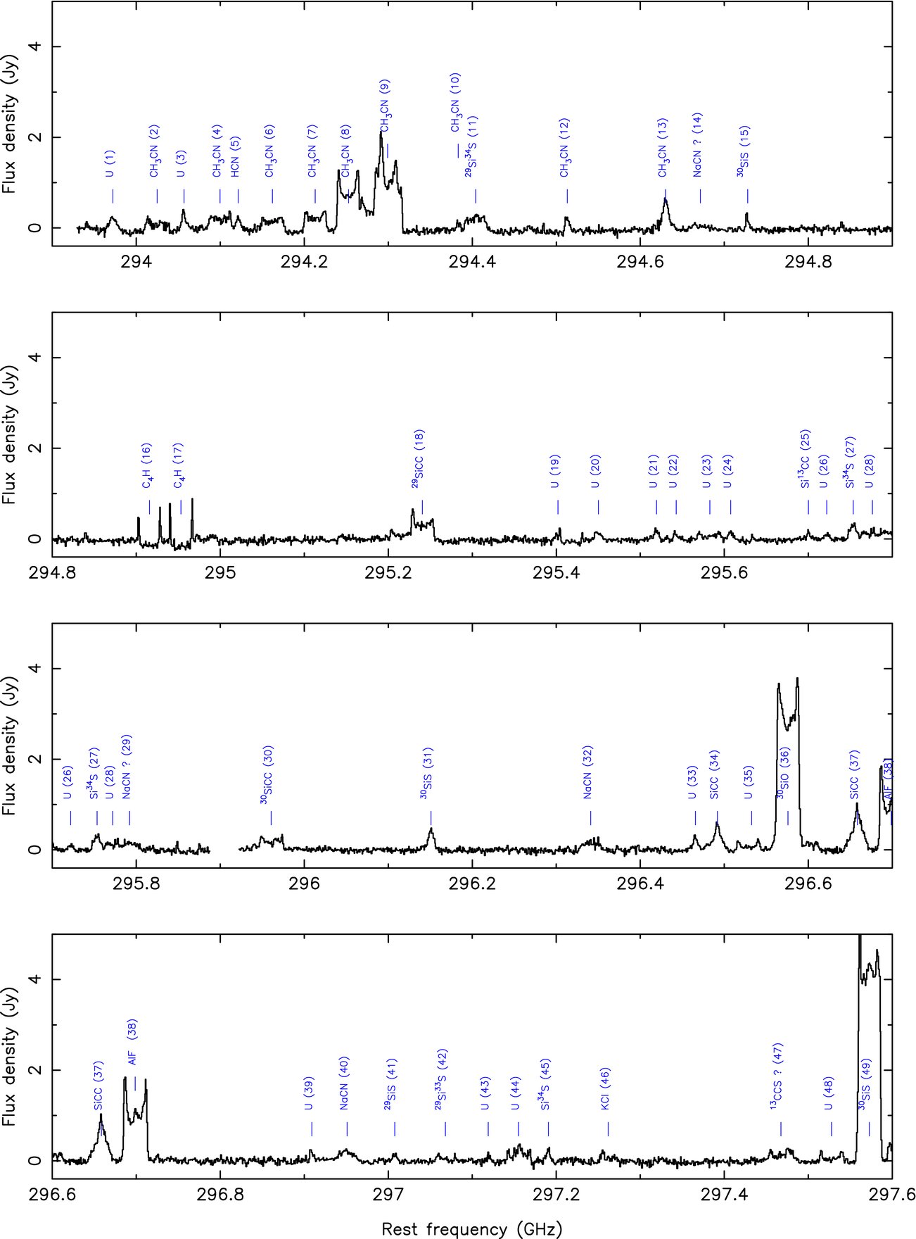
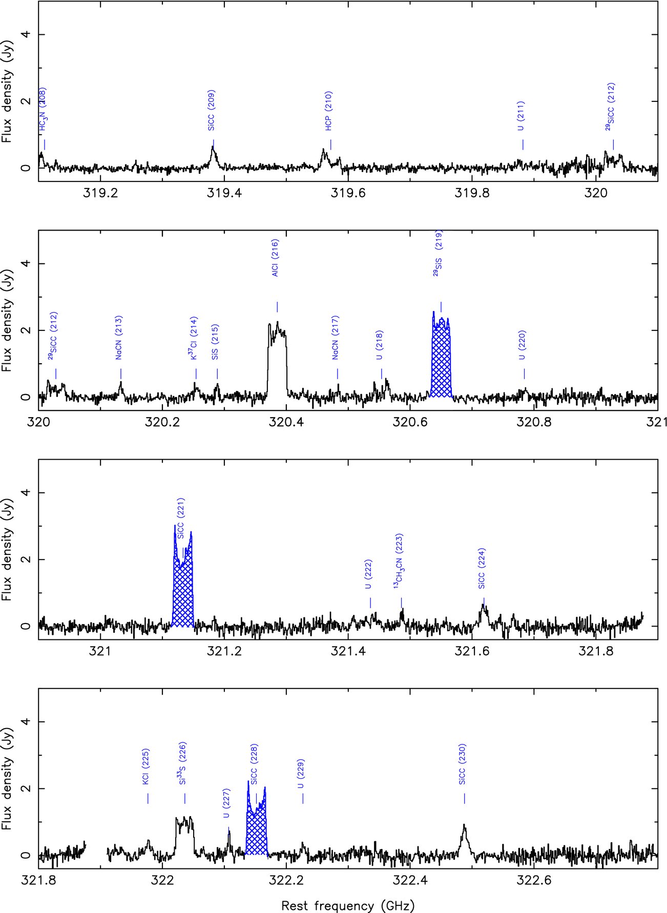
Figure 13. Expansion velocity as a function of radius. The black curve is from Keady & Ridgway (1993). A subset of 71 out of 442 observed lines which have reliable measurements of Vexp and de-convolved angular sizes were plotted. See the text for details. The red curve is a plot of Equation (2).
Download figure:
Standard image High-resolution image
Also shown in Figure 13 are theoretical velocity profiles. The black curve is the assumed velocity profile used as a model for the analysis of observed infrared molecular lines by Keady & Ridgway (1993, see their Figure 3(a)). The red curve shows the velocity profile given by

where v∞ is the terminal velocity of 14 km s−1 and θ0 is the dust formation radius of 013 as assumed by Kwan & Linke (1982). Figure 13 suggests a larger value of θ0 ≈ 05.
6. CONCLUSIONS
The SMA line survey of IRC+10216 has yielded 442 lines, 293 of which have been assigned to known transitions. Most are from molecules known to exist in the CSE of IRC+10216, including, SiCC, SiS, SiO, CS, C4H, CH3CN, HCN, HC3N, and their isotopic species. Also detected are several lines from salts and metals, including, NaCl, KCl, AlCl, and AlF. More than 100 lines remain unidentified. Maps of these U lines typically show very compact emission, suggesting vibrationally excited lines of known simple molecules, produced very close to the star or even within its photosphere. Assignment of the substantial number of unidentified lines observed in the inner envelope awaits laboratory measurements of rotational transitions from high lying levels in the ground and vibrationally excited states of polyatomic molecules.
We are grateful to Raymond Blundell, SMA director, for his encouragement and support throughout the course of this project. We thank the anonymous referee for a careful review of the manuscript and several helpful comments.
Footnotes
- 7
The Submillimeter Array is a joint project between the Smithsonian Astrophysical Observatory and the Academia Sinica Institute of Astronomy and Astrophysics, and is funded by the Smithsonian Institution and the Academia Sinica.
- 8
- 9
See http://iram.fr/IRAMFR/GILDAS for more information about GILDAS software.
- 10
The CDMS catalogue at http://www.ph1.uni-koeln.de/vorhersagen/.
- 11
The JPL catalogue at http://spec.jpl.nasa.gov/home.html.
- 12
The Lovas line list at http://physics.nist.gov/PhysRefData/Micro/Html/contents.html.
- 13
CASSIS has been developed by CESR-UPS/CNRS(http://cassis.cesr.fr).
- 14