


ABSTRACT
We present a catalog of high-energy gamma-ray sources detected by the Large Area Telescope (LAT), the primary science instrument on the Fermi Gamma-ray Space Telescope (Fermi), during the first 11 months of the science phase of the mission, which began on 2008 August 4. The FirstFermi-LAT catalog (1FGL) contains 1451 sources detected and characterized in the 100 MeV to 100 GeV range. Source detection was based on the average flux over the 11 month period, and the threshold likelihood Test Statistic is 25, corresponding to a significance of just over 4σ. The 1FGL catalog includes source location regions, defined in terms of elliptical fits to the 95% confidence regions and power-law spectral fits as well as flux measurements in five energy bands for each source. In addition, monthly light curves are provided. Using a protocol defined before launch we have tested for several populations of gamma-ray sources among the sources in the catalog. For individual LAT-detected sources we provide firm identifications or plausible associations with sources in other astronomical catalogs. Identifications are based on correlated variability with counterparts at other wavelengths, or on spin or orbital periodicity. For the catalogs and association criteria that we have selected, 630 of the sources are unassociated. Care was taken to characterize the sensitivity of the results to the model of interstellar diffuse gamma-ray emission used to model the bright foreground, with the result that 161 sources at low Galactic latitudes and toward bright local interstellar clouds are flagged as having properties that are strongly dependent on the model or as potentially being due to incorrectly modeled structure in the Galactic diffuse emission.
Export citation and abstract BibTeX RIS
1. INTRODUCTION
The Fermi Gamma-ray Space Telescope has been routinely surveying the sky with the Large Area Telescope (LAT) since the science phase of the mission began in 2008 August. The combination of deep and fairly uniform exposure, good per-photon angular resolution, and stable response of the LAT has made for the most sensitive, best-resolved survey of the sky to date in the 100 MeV to 100 GeV energy range.
Observations at these high energies reveal non-thermal sources and a wide range of processes by which particles are accelerated. The utility of a uniformly analyzed catalog such as this is both for identifying special sources of interest for further study and for characterizing populations of γ-ray emitters. The LAT survey data analyzed here allow much more detailed characterizations of variability and spectral shapes than has been possible before.
Here we expand on the Bright Source List (BSL; Abdo et al. 2009m), which was an early release of 205 high-significance (likelihood Test Statistic TS>100; see Section 4.3) sources detected with the first 3 months of science data. The expansion is in terms of time interval considered (11 months versus 3 months), energy range (100 MeV–100 GeV versus 200 MeV–100 GeV), significance threshold (TS>25 versus TS>100), and detail provided for each source. Regarding the latter, we provide elliptical fits to the confidence regions for source location (versus radii of circular approximations), fluxes in five bands (versus 2 for the BSL) for the range 100 MeV–100 GeV, and monthly light curves for the integral flux over that range.
We also provide associations with previous γ-ray catalogs, for EGRET (Hartman et al. 1999; Casandjian & Grenier 2008) and AGILE (Pittori et al. 2009), and with likely counterpart sources from known or suspected source classes. The number of sources for which no plausible associations are found is 630, at the specified confidence level for source association (80%). The First LAT AGN Catalog (1LAC; Abdo et al. 2010l) is based on the 1FGL sources, and applies the same association methods, but provides associations for active galactic nuclei (AGNs) down to the 50% confidence level.
As with the BSL, the First Fermi-LAT catalog of γ-ray sources (1FGL, for first Fermi Gamma-ray LAT) is not flux limited and hence not uniform. As described in Section 4, the sensitivity limit depends on the region of the sky and on the hardness of the spectrum. Only sources with TS> 25 (corresponding to just over 4σ statistical significance) are included, as described below.
2. GAMMA-RAY DETECTION WITH THE LARGE AREA TELESCOPE
The LAT is a pair-production telescope (Atwood et al. 2009). The tracking section has 36 layers of silicon
strip detectors to record the tracks of charged particles, interleaved with 16
layers of tungsten foil (12 thin layers, 0.03 radiation length, at the top or
Front of the instrument, followed by four thick layers, 0.18
radiation length, in the Back section) to promote γ-ray pair
conversion. Beneath the tracker is a calorimeter comprised of an eight-layer array
of CsI crystals (1.08 radiation length per layer) to determine the γ-ray energy. The
tracker is surrounded by segmented charged-particle anticoincidence detectors
(plastic scintillators with photomultiplier tubes) to reject cosmic-ray background
events. The LAT's improved sensitivity compared to EGRET stems from a large peak
effective area (∼8000 cm2, or ∼six times greater than EGRET's), large
field of view (∼2.4 sr, or nearly five times greater than EGRET's), good background
rejection, superior angular resolution (68% containment angle ∼0 6 at 1 GeV for the
Front section and about a factor of 2 larger for the
Back section versus ∼17 at 1 GeV for EGRET; Thompson et al.
1993), and improved observing
efficiency (keeping the sky in the field of view with scanning observations versus
inertial pointing for EGRET). Pre-launch predictions of the instrument performance
are described in Atwood et al. (2009).
6 at 1 GeV for the
Front section and about a factor of 2 larger for the
Back section versus ∼17 at 1 GeV for EGRET; Thompson et al.
1993), and improved observing
efficiency (keeping the sky in the field of view with scanning observations versus
inertial pointing for EGRET). Pre-launch predictions of the instrument performance
are described in Atwood et al. (2009).
The data analyzed for the 1FGL catalog were obtained during 2008 August 4–2009 July 4 (LAT runs 239557414 through 268411953, where the numbers refer to the Mission Elapsed Time (MET) in seconds since 00:00 UTC on 2001 January 1, at the start of the data acquisition runs). During most of this time Fermi was operated in sky-scanning survey mode (viewing direction rocking 35° north and south of the zenith on alternate orbits). During May 7–20 the rocking angle was increased to 39° for operational reasons. In addition, a few hours of special calibration observations during which the rocking angle was much larger than nominal for survey mode or the configuration of the LAT was different from normal for science operations were obtained during the period analyzed. Time intervals when the rocking angle was larger than 43° have been excluded from the analysis, because the bright limb of the Earth enters the field of view (see below).
In addition, two short time intervals associated with bright γ-ray bursts (GRBs) that were detected in the LAT have been excluded: MET 243216749–243217979 (GRB080916C Abdo et al. 2009k) and MET 263607771–263625987 (GRB090510 Abdo et al. 2009a). With these intervals removed, the GRBs and their afterglows cannot affect the detection and characterization of nearby sources.
Observations were nearly continuous during the survey interval, although a few data gaps are present due to operational issues, special calibration runs, or in rare cases, data loss in transmission. Table 1 lists all data gaps longer than 1 hr. The longest gap by far is 3.9 days starting early on March 16; together the gaps longer than 1 hr amount to ∼7.9 days or 2.4% of the interval analyzed for the 1FGL Catalog.
Table 1. Gaps Longer Than 1 hr in Data
| Start of Gap (UTC) | Duration (hr) |
|---|---|
| 2008 Sep 30 14:27 | 1.16 |
| 2008 Oct 11 03:14 | 1.59 |
| 2008 Oct 11 11:04 | 3.82 |
| 2008 Oct 14 12:23 | 3.83 |
| 2008 Oct 14 17:11 | 3.49 |
| 2008 Oct 14 20:22 | 1.59 |
| 2008 Oct 15 17:03 | 3.47 |
| 2008 Oct 16 15:18 | 1.83 |
| 2008 Oct 22 19:20 | 1.59 |
| 2008 Oct 22 23:43 | 2.06 |
| 2008 Oct 23 11:16 | 1.91 |
| 2008 Oct 30 16:43 | 1.59 |
| 2008 Dec 11 17:41 | 6.37 |
| 2009 Jan 1 00:35 | 1.72 |
| 2009 Jan 6 20:43 | 6.98 |
| 2009 Jan 13 13:26 | 2.10 |
| 2009 Jan 17 12:58 | 2.05 |
| 2009 Jan 28 19:28 | 4.78 |
| 2009 Feb 1 15:46 | 1.59 |
| 2009 Feb 15 10:15 | 1.05 |
| 2009 Mar 16 00:27 | 116.78 |
| 2009 May 2 19:04 | 8.94 |
| 2009 May 7 15:21 | 5.46 |
| 2009 Jun 26 12:59 | 3.19 |
Download table as: ASCIITypeset image
The total live time included is 245.6 days (21.22 Ms). This corresponds to an absolute efficiency of 73.5%. Most of the inefficiency is due to time lost during passages through the South Atlantic Anomaly (∼13%) and to readout dead time (9.2%).
The standard onboard filtering, event reconstruction, and classification were applied to the data (Atwood et al. 2009), and for this analysis the "Diffuse" event class71 is used. This is the class with the least residual contamination from charged-particle background events, released to the public. The tradeoff for using this event class relative to the "looser" Source class is a primarily reduced effective area, especially below 500 MeV.
The instrument response functions (IRFs)—effective area, energy redistribution, and
point-spread function (PSF)—used in the likelihood analyses described below were
derived from GEANT4-based Monte Carlo simulations of the LAT using the
event-selection criteria corresponding to the Diffuse event class. The Monte Carlo
simulations themselves were calibrated prior to launch using accelerator tests of
flight-spare "towers" of the LAT (Atwood et al. 2009) and have since been updated based on
observation of pileup effects on the reconstruction efficiency in flight data (Rando
et al. 2009). The effect introduces
an inefficiency that is proportional to the trigger rate and dependent on energy.
The likelihood analysis for characterizing the sources uses the P6_V3 IRFs (see
Section 4.3), which have the
effective areas corrected for the inefficiency corresponding to the overall average
trigger rate seen by the LAT. The use of the P6_V3 IRFs allows the energy range of
the analysis for the catalog to be extended down to 100 MeV (versus 200 MeV for the
BSL analysis, which used P6_V1). Below 100 MeV, the effective area is relatively
small and strongly dependent on energy. These considerations, together with the
increasing breadth of the PSF at low energies (scaling approximately as
08(E/1 GeV)−0.8), motivated the selection of 100
MeV as the lower limit for this analysis.
The alignment of the Fermi observatory viewing direction with the z-axis of the LAT was found to be stable during survey-mode observations (Abdo et al. 2009q). Analyses of flight data suggest that the PSF is somewhat broader than the calculated Diffuse class PSF at energies greater than ∼10 GeV; the primary effect on the current analysis is to decrease the localization capability somewhat. As discussed below, this is taken into account in the catalog by increasing the derived sizes of source location regions by 10%.
For the analysis, a cut on zenith angle (angle between the boresight of the LAT and the local zenith) at 105° was applied to the Diffuse class events to limit the contamination from albedo γ-rays from interactions of cosmic rays with the upper atmosphere of the Earth. These interactions make the limb of the Earth (zenith angle ∼113° at the 565 km, nearly circular orbit of Fermi) an intensely bright γ-ray source (Thompson et al. 1981). The limb is a very far-off axis in survey-mode observations, at least 70° for the data set considered here because of the rocking angle requirement described above. Removing events at zenith angles greater than 105° affects the exposure calculation negligibly but reduces the overall background rate. After these cuts, the data set contains 1.1 × 10⁷ Diffuse class events with energies >100 MeV.
The intensity map of Figure 1 summarizes the data set used for this analysis and shows the dramatic increase of the brightness of the γ-ray sky at low Galactic latitudes. The corresponding exposure is relatively flat and featureless as was the case for the shorter time interval analyzed for the BSL. The degree of exposure nonuniformity is relatively small (about 30% difference between minimum and maximum), with the deficit around the south celestial pole due to loss of exposure during passages of Fermi through the South Atlantic Anomaly (Atwood et al. 2009).

Figure 1. Sky map of the LAT data for the time range analyzed in this paper, Aitoff projection in Galactic coordinates. The image shows γ-ray intensity for energies >300 MeV, in units of photons m−2 s−1 sr−1.
Download figure:
Standard image High-resolution image3. DIFFUSE EMISSION MODEL
An essential input to the analyses for detecting and characterizing γ-ray sources in the LAT data is a model of the diffuse γ-ray intensity of the sky. Interactions between cosmic rays and interstellar gas and photons make the Milky Way a bright, structured celestial foreground. Unresolved emission from extragalactic sources contributes an isotropic component as well. In addition, residual charged-particle background, i.e., cosmic rays that trigger the LAT and are misclassified as γ-rays, provides another approximately isotropic background. For the analyses described in this paper we used models for the Galactic diffuse emission (gll_iem_v02.fit) and isotropic backgrounds that were developed by the LAT team and made publicly available as models recommended for high-level analyses. The models, along with descriptions of their derivation, are available from the Fermi Science Support Center.72
Briefly, the model for the Galactic diffuse emission was developed using spectral line surveys of H i and CO (as a tracer of H2) to derive the distribution of interstellar gas in Galactocentric rings. Infrared tracers of dust column density were used to correct column densities as needed, e.g., in directions where the optical depth of H i was either over- or underestimated. The model of the diffuse γ-ray emission was then constructed by fitting the γ-ray emissivities of the rings in several energy bands to the LAT observations. The fitting also required a model of the inverse Compton emission that was calculated using GALPROP (Strong et al. 2004, 2007) and a model for the isotropic diffuse emission.
The isotropic component was derived as the residual of a fit of the Galactic diffuse emission model to the LAT data at Galactic latitudes above |b| = 30° and so by construction includes the contribution of residual (misclassified) cosmic rays for the event analysis class used (Pass 6 Diffuse; see Section 2). Treating the residual charged particles effectively as an isotropic component of the γ-ray sky brightness rests on the assumption that the acceptance for residual cosmic rays is the same as for γ-rays. This approximation has been found to be acceptable; the numbers of residual cosmic-ray background events scale as the overall live time and any acceptance differences from γ-rays would not introduce a small-scale structure in the models for likelihood analysis.
4. CONSTRUCTION OF THE CATALOG
The procedure used to build the 1FGL catalog follows the same steps described in Abdo et al. (2009m) for the BSL, with a number of improvements. We review those steps in this section, highlighting what was done differently for 1FGL.
Three steps were applied in sequence: detection, localization, and significance estimation. In this scheme, the threshold for inclusion in 1FGL is defined at the last step, but the completeness is controlled by the first one. After the list was defined we determined the source characteristics (flux in five energy bands, time variability). The 1FGL catalog includes much more information for each source than the BSL. In what follows, flux F means photon flux and spectral index Γ is for photons (i.e., F ∝ E−Γ).
In constructing the catalog the source detection step was applied only to the data from the full 11 month period as a whole. That is to say, we did not search for potentially flaring sources which might only be detectable on shorter timescales. Independently of this work, the LAT Automated Science Processing (Atwood et al. 2009) and Flare Advocate activity provide a framework through which such flaring sources are detected in a timely manner and reported as Astronomer's Telegrams (ATels). However, since all bright flaring sources that were reported as ATels were also bright enough to be detected over 11 months based on their average fluxes, they are included in the 1FGL catalog anyway.
The pulsars (Abdo et al. 2010m) and X-ray binaries (Abdo et al. 2009j, 2009n, 2009p) which are identified via their rotation or orbital period, were detected and localized as ordinary sources. But they were entered explicitly at their true positions in the main maximum likelihood analysis (Section 4.3), in order not to bias their characteristics and those of their surroundings if the Galactic diffuse model is imperfect (Section 3). For the LAT-detected pulsars, we used the radio or γ-ray timing localization (Abdo et al. 2010m) which is always more precise than that based on the spatial distribution of the events. We have checked that the positions of the brightest pulsars found by the localization algorithm (Section 4.2) were consistent with their true positions at the 95% level (using only the statistical error, without any systematic correction).
4.1. Detection
The detection step used the same ideas that were detailed in Abdo et al. (2009m). It was based on the same three energy bands, combining Front and Back events to preserve spatial resolution. The detection does not use events below 200 MeV, which have poor angular resolution. It uses events up to 100 GeV. The full band (6.7 × 10⁶ counts) starts at 200 MeV for Front and 400 MeV for Back events. The medium band (12.0 × 10⁵ counts) starts at 1 GeV for Front and 2 GeV for Back events. The hard band (10.7 × 10⁴ counts) starts at 5 GeV for Front and 10 GeV for Back events.
We used the same partitioning of the sky into 24 planar projections as in the
BSL, and the same two wavelet-based detection methods:
mr_filter (Starck & Pierre 1998) and PGWave (Damiani et al.
1997; Ciprini et al. 2007). The methods looked for
sources on top of the diffuse emission model described in Section 3. For mr_filter
the threshold was set in each image using the False Discovery Rate procedure
(Benjamini & Hochberg 1995)
at 5% of false detections. For PGWave we used a flat threshold
at 4σ. For comparison with the BSL, the number of "seed" sources from
mr_filter was 857 in the full band, 932 in the medium band,
and 331 in the hard band. Contrary to the BSL procedure, we combined the results
of those two methods (eliminating duplicates) rather than choosing a baseline
method and using the other for comparison. The rationale was to limit the number
of missed sources to a minimum, since the later steps do not introduce any
additional sources. Duplicates were defined after the first localization
(pointfit in Section 4.2, run separately on each list of seeds). If
two resulting positions were consistent within the quadratic sum of 95% error
radii only one source was kept (that with highest significance estimate). Where
pointfit did not converge, the 95% error radius was set to
03, typical for faint sources (Section 4.2).
To that same end we also introduced for 1FGL two other detection methods.
- 1.Point find, a tool that searches for candidate point sources by maximizing the likelihood function for trial point sources at each direction in a HEALPix (Górski et al. 2005) order 9 (pixel size ∼0.1 deg2) tessellation of the sky. The algorithm for evaluating the likelihood is optimized for speed by using energy-dependent binning of the photon data, choosing four energy bands per decade starting at 700 MeV, and a HEALPix order commensurate with the PSF width in each band. A first pass examines the significance of a trial point source at the center of each pixel, on the assumption that the diffuse background is adequately described by the model for Galactic diffuse emission and ignoring any nearby point sources. The likelihood is optimized with respect to the signal fraction (i.e., the source and diffuse intensities are not fit separately) in each energy band, with the total likelihood being the product over all the bands. This makes the result independent of the spectrum of the point source or of the diffuse background. While the search is quite efficient, it produces many false signals, so a second pass is used to optimize a more detailed likelihood function which includes nearby detected sources and fits the test source flux and diffuse background normalization independently. The result of the second pass is a map of TS from which the coordinates of candidate point sources can be derived.
- 2.The minimum spanning tree (Campana et al. 2008) looks for clusters of high-energy events (>4 GeV outside the Galactic plane and >10 GeV at |b| < 15°). It is restricted to high energies because it does not account for structured background, but can efficiently detect very hard sources.
We combined the "seed" positions from those two methods with those from the wavelet-based methods, using the same procedure for removing duplicates as above.
Finally, we introduced external seeds from the BZCAT (Massaro et al. 2009) and WMAP (Wright et al. 2009) catalogs. The BZCAT catalog is not homogeneous but includes the great majority of known, well-characterized blazars. It is a superset of the CGRaBS (Healey et al. 2008) catalog and has broader sky coverage. The WMAP catalog includes mainly bright FSRQ blazars, and was used primarily to try to recover soft-spectrum sources that might have been missed by the source-detection algorithms.
In order to not bias the 1FGL catalog toward those external sources, we used them as seeds only when there was no seed from the detection methods within its 95% error radius. Of the 335 BZCAT seeds introduced, 24 survived as LAT γ-ray sources in this catalog. Of the seven WMAP seeds, three remain in the catalog.
The variety of seeds that we used means that the catalog is not homogeneous. Because of the strong underlying diffuse emission, achieving a truly homogeneous catalog was not possible in any case. Our aim was to provide enough seeds to allow the main maximum likelihood analysis (Section 4.3) to be the defining step of the catalog construction. The total number of seeds was 2433.
4.2. Localization
The localization of faint or soft sources is more sensitive to the diffuse emission and to nearby sources than for brighter sources, so we proceeded in three steps instead of just one for the bright sources considered in the BSL.
- 1.The first step consisted of localizing the sources before the main maximum likelihood analysis (Section 4.3) as we did for the BSL (using pointfit), treating each source independently but in descending order of significance and incorporating the bright sources into the background for the fainter ones. This is fast and provides a good enough starting point for step 2.
- 2.The second step consisted of improving the localization within the main maximum likelihood analysis (Section 4.3) using the gtfindsrc utility in the Science Tools.73 Again sources are considered in descending order of significance. When localizing one source, the others are fixed in position, but the fluxes and spectral indices of sources within 2° are left free to accommodate the loss of low-energy photons in the model if the source that is being localized moves away. At the end of that step we have a good representation of the location, flux, and spectral shape of the sources over the entire sky, but a single error radius to describe the error box.
- 3.The third step is new and described in more detail below. It uses a similar framework as the first step, but incorporates the results of the main maximum likelihood analysis for all sources other than the one being considered, so it has a good representation of the source's surroundings. It is faster than gtfindsrc and gttsmap and returns a full TS map around each source and an elliptical representation as well as an indicator of the quality of the elliptical fit.
The first and third steps used a likelihood analysis tool (pointfit) that provides speed at little sacrifice of precision by maximizing a specially constructed binned likelihood function. Photons are assigned to 12 energy bands (four per decade from 100 MeV–100 GeV) and HEALpix-based spatial bins for which the size is selected to be small compared with the scale set by the PSF. Since the PSF for Front-converting photons is significantly smaller than that for Back conversions, there are separate spatial bins for Front and Back. Note that the width of the PSF at a given energy is only a weak function of incidence angle. For pointfit the likelihood function is evaluated using the PSF averaged over the full field of view for each energy band. For each band, we define the likelihood as a function of the position and flux of the assumed point source, and adopt as the background the sum of Galactic diffuse, isotropic diffuse (see Section 3), and any nearby (i.e., within 5°), other point sources in the catalog. The flux for each band is then evaluated by maximizing the likelihood of the data given the model using the coordinates defined by gtfindsrc. The overall likelihood function, as a function of the source position, is then the product of the band likelihoods. We define a function of the position p, as 2(log(Lmax) − log(L(p)), where L is the likelihood function described above. This function, according to Wilks' theorem (Wilks 1938), is the probability distribution for the coordinates of the point source consistent with the observed data. Note that the width of this distribution is a measure of the uncertainty, and that it scales directly with the width of the PSF.
We then fit the distribution to a two-dimensional quadratic form with five parameters describing the expected elliptical shape: the coordinates (R.A. and decl.) of the center of the ellipse, semimajor and semiminor axis extents (α and β), and the position angle ϕ of the ellipse.74 A "quality" factor is evaluated to represent the goodness of the fit: it is the square root of the sum of the squares of the deviations for eight points sampled along the contour where the value is expected to be 4.0, that is, 2σ from the maximum likelihood coordinates of the source.
We quote the parameters of the ellipse that would contain 95% of the probability for the location of the source; for Gaussian errors this would be a radius of 2.45σ. An analysis of the deviations of 396 AGNs at high latitudes from the positions of the nearest LAT point sources indicated that the PSF width is underestimated, on average, by a factor of 1.10 ± 0.05. Thus the final uncertainties reported by pointfit were scaled up by a factor of 1.1. To visually assess the fits, a TS map was made for each source, and these were considered in evaluating the analysis flags that are discussed in Section 4.8.
Twelve sources either did not converge at the third step, converged to a point far away (>1°), or were in crowded regions where the procedure (which does not have free parameters for the fluxes of nearby sources) may not be reliable. Those 12 were left at their gtfindsrc positions. They can be easily identified in the 1FGL catalog because they have identical semimajor and semiminor axes for the source location uncertainty and position angle 0. The LAT-detected pulsars and X-ray binaries, which were placed at the high-precision positions of these identified sources, have null values in the localization parameters.
Figure 2 illustrates the resulting position errors as a function of the TS values obtained in Section 4.3. The relatively large dispersion that is seen at a given TS is in part due to the local conditions (level of diffuse γ-ray emission) but primarily depends upon the source spectrum. Hard-spectrum sources are better localized than soft ones for the same TS (Figure 3) because the PSF is so much narrower at high energy. At our threshold of TS = 25, the typical 95% position error is about 10' and most 95% errors are below 20'.

Figure 2. 95% source location error (geometric mean of the two axes of the ellipse) as a function of TS (Section 4.3). The dashed line is a (TS)−0.4 trend for reference (not adjusted vertically).
Download figure:
Standard image High-resolution image
Figure 3. 95% source location error multiplied by (TS)0.4 to remove the global trend (Figure 2) as a function of the photon spectral index from Section 4.3.
Download figure:
Standard image High-resolution image4.3. Significance and Thresholding
The detection and localization steps provide estimates of source significances. However, since the detection step does not use the energy information and the localization step fits only one source at a time, these estimates are not sufficiently accurate for use in the catalog. To better estimate the source significances, we use a three-dimensional maximum likelihood algorithm (gtlike) in unbinned mode (i.e., the position and energy of each event is considered individually) applied on the full energy range from 100 MeV–100 GeV using the P6_V3 IRFs (see Section 2). This is part of the standard Science Tools software package, currently at version 9r15p5. The tool does not vary the source position, but does adjust the source spectrum. The underlying optimization engine is Minuit.75 The code works well with up to ∼30 free parameters, an important consideration for regions where sources are close enough together to partially overlap. The gtlike tool provides the best-fit parameters for each source and the Test Statistic TS = 2Δlog(likelihood) between models with and without the source. The TS associated with each source is a measure of the source significance. Error estimates (and a full covariance matrix) are obtained from Minuit in the quadratic approximation around the best fit. For this stage we modeled the sources with simple power-law spectra. It should be noted that gtlike does not include the energy dispersion in the TS calculation (i.e., it assumes that the measured energy is the true energy). Given the 8% to 10% energy resolution of the LAT over the wide energy bands used in the present analyses, this approximation is justified.
Because the fitted fluxes and spectra of the sources can be very sensitive to even slight errors in the spectral shape of the diffuse emission we allow the Galactic diffuse model (Section 3) to be corrected (i.e., multiplied) locally by a power law in energy with free normalization and spectral slope. The slope varies between 0 and 0.07 (making it harder) in the Galactic plane and the normalization by ±10% (down from 0.15% and 20% for the BSL). The smaller excursions of that corrective slope when compared to the BSL reflect the better fit of the current diffuse model to the data. The normalization of the isotropic component of the diffuse emission (which represents the extragalactic and residual backgrounds) was left free. The three free parameters were separately adjusted in each region of interest (RoI).
We split the sky into overlapping circular RoIs. The parameters are free for sources in the central part of each RoI (RoI radius minus 7°), such that all free sources are well within the RoI even at low energy (7° is larger than r68 at 100 MeV). It is advantageous (for the global convergence over the entire sky) to use large RoIs, but at the same time smaller RoIs allow spectral variations of the diffuse emission relative to the model to be corrected in more detail. We set the RoI sizes so that not more than eight sources are free at a time. Adding three parameters for the diffuse model, the total number of free parameters in each RoI is normally 19 at most. We needed 445 RoIs to cover the 2433 seed positions. The RoI radii range between 9° and 15°.
We proceed iteratively. All RoIs are processed in parallel and a global current model is assembled after each step in which the best-fit parameters for each source are taken from the RoI whose center is closest to the source. The local model for each RoI includes sources up to 7° outside the RoI (which can contribute at low energy due to the broad PSF). Their parameters are fixed to their values in the global model at the previous step. The parameters of the sources inside the RoI but within 7° of the border are also fixed except in two cases (not considered for the BSL analysis).
- 1.Sources within 2° of any source inside the central part, because they can influence the inner source. 2° is chosen to be larger than twice the containment radius at 1 GeV (2 × 08) where the LAT sensitivity
peaks (Figure 18).
We leave both flux and spectral index free for these.
- 2.Very bright sources contributing more than 5% of the total counts in the RoI because they can influence the diffuse emission parameters. We leave only the flux free for these.
All seed sources start at 0 flux at the first step; the starting point for the slope is 2. We iterate over five steps; the fits change very little after the fourth. To facilitate the convergence the seed sources are not entered all at once. The brightest 10% of the sources are entered at the first step, 30% at the second step, and finally all at the third step. At each step we remove seed sources with low TS, raising the threshold for inclusion into the global model from 10 at the third step to 15 at the fourth and finally 25 at the last step. All seeds are reentered at the fourth step to avoid losing faint sources before the global model has fully converged. We have checked via simulations that removing the faint sources has little impact on the bright ones, much less than changing the diffuse model (Section 4.6). This procedure left 1451 sources above threshold. The variation of the detection threshold across the sky and the dependence of the threshold on source spectrum are discussed in Appendix A.
The TS of each source can be related to the probability that such an excess can be obtained from background fluctuations alone. The probability distribution in such a situation (source over background) is not known precisely (Protassov et al. 2002). However since we consider only positive fluctuations, and each fit involves four degrees of freedom (two for position, plus flux and spectral index), the probability to get at least TS at a given position in the sky is close to 1/2 of the χ2 distribution with four degrees of freedom (Mattox et al. 1996), so that TS = 25 corresponds to a false detection probability of 2.5 × 10⁻⁵ or 4.1σ (one sided). For the BSL we considered only two degrees of freedom because the localization was based on a simpler algorithm which did not involve explicit minimization of the same likelihood function.
The sources that we see are best (most strongly) detected around 1 GeV. This is
approximately the median of the Pivot_Energy quantity in the catalog, i.e., the
energy at which the uncertainties in normalization and spectral index for the
power-law fit are uncorrelated. At 1 GeV, the 68% containment radius is
approximately r68 = 08. The number of independent
elements in the sky (trials factor) is about
4π/(πr268) in which
r68 is converted to radians. This is about 2 ×
104 so at a threshold of TS = 25 we expect less than 1 spurious
source by chance only. If any, there might be a few very hard spurious sources
in the catalog because hard sources have a smaller effective PSF so that the
trial factor is larger. The main reason for potentially spurious sources,
though, is our imperfect knowledge of the underlying diffuse emission (Section
4.6).
4.4. Flux Determination
The maximum likelihood method described in Section 4.3 provides good estimates of the source significances and the overall spectral slope, but not very accurate estimates of the fluxes. This is because the spectra of most sources do not follow a single power law over that broad energy range (three decades). Within the two most populous categories, the AGNs often have broken power-law spectra and the pulsars have power-law spectra with an exponential cutoff. In both cases fitting a single power law over the entire range overpredicts the flux in the low-energy region of the spectrum, which contains the majority of the photons from the source, biasing the fluxes high. On the other hand, the effect on the significance is low due to the broad PSF and high background at low energies.
In addition, the significance is mostly obtained from GeV photons (Figure 18) whereas the photon flux in the full range (above 100 MeV) is dominated by lower energy events so that the uncertainty on that flux can be quite large even for highly significant sources. For example, the typical relative uncertainty on the photon flux above 100 MeV is 23% for a TS = 100 source with spectral index 2.2.
To provide better estimates of the source fluxes, we decided to split the range into five energy bands from 100 to 300 MeV, 300 MeV to 1 GeV, 1 to 3 GeV, 3 to 10 GeV, and 10 to 100 GeV (the number of counts does not justify dividing the last decade into two bands). The list of sources remained the same in all bands. It is generally not possible to fit the spectral index in each of those relatively narrow energy bands (and the flux estimate does not depend very much on the index), so we simply froze the spectral index of each source to the best fit over the full interval. The spectral bias to the Galactic diffuse emission (Section 4.3) was also frozen.
The estimate from the sum of the five bands is on average within 30% of the flux obtained from the global power-law fit (as described in Section 2, with excursions up to a factor of 2). We have also compared those estimates with a more precise spectral model for the three bright pulsars (Vela, Geminga, and the Crab). The sum of the five fluxes is within 5% of the more precise flux estimate, whereas the power-law estimate is 25% too high for Vela and Geminga. However because the flux in each band is not constrained globally as in the power-law model, the relative uncertainty of the sum of the five fluxes is even larger than that for the power-law fit, typically 50% for a TS = 100 source with spectral index 2.2. For that reason we do not show this very poorly measured quantity in Table 2. We provide instead the photon flux between 1 and 100 GeV (the sum of the three high energy bands), which is much better defined. The relative uncertainty on this flux is typically 18% for a TS = 100 source with spectral index 2.2.
Table 2. LAT 1FGL Catalog
| Name 1FGL | R.A. | Decl. | l | b | θ1 | θ2 | ϕ | σ | F35 | ΔF35 | S25 | ΔS25 | Γ25 | ΔΓ25 | Curv. | Var. | Flags | γ-ray Assoc. | TeV | Class | ID or Assoc. | Ref. |
|---|---|---|---|---|---|---|---|---|---|---|---|---|---|---|---|---|---|---|---|---|---|---|
| J0000.8+6600c | 0.209 | 66.002 | 117.812 | 3.635 | 0.112 | 0.092 | −73 | 9.8 | 2.9 | 0.6 | 35.2 | 5.7 | 2.60 | 0.09 | ... | ... | 6 | ... | ... | ... | ... | ... |
| J0000.9−0745 | 0.236 | −7.763 | 88.903 | −67.237 | 0.179 | 0.130 | 16 | 5.6 | 1.0 | 0.0 | 9.2 | 3.0 | 2.41 | 0.20 | ... | ... | ... | ... | ... | bzb | CRATES J0001−0746 | ... |
| J0001.9−4158 | 0.482 | −41.982 | 334.023 | −72.028 | 0.121 | 0.116 | 53 | 5.5 | 0.5 | 0.2 | 14.4 | 0.0 | 1.92 | 0.25 | ... | ... | ... | ... | ... | ... | ... | ... |
| J0003.1+6227 | 0.798 | 62.459 | 117.388 | 0.108 | 0.119 | 0.112 | −19 | 7.8 | 2.1 | 0.5 | 19.9 | 4.9 | 2.53 | 0.10 | T | ... | 3 | ... | ... | ... | ... | ... |
| J0004.3+2207 | 1.081 | 22.123 | 108.757 | −39.448 | 0.183 | 0.157 | 58 | 4.7 | 0.6 | 0.2 | 5.3 | 2.5 | 2.35 | 0.21 | ... | ... | ... | ... | ... | ... | ... | ... |
| J0004.7−4737 | 1.187 | −47.625 | 323.864 | −67.562 | 0.158 | 0.148 | −5 | 6.6 | 0.8 | 0.3 | 10.9 | 3.3 | 2.56 | 0.17 | ... | ... | ... | ... | ... | bzq | PKS 0002−478 | ... |
| J0005.1+6829 | 1.283 | 68.488 | 118.689 | 5.999 | 0.443 | 0.307 | −4 | 6.1 | 1.4 | 0.5 | 17.0 | 4.8 | 2.58 | 0.12 | ... | ... | 1,4 | ... | ... | ... | ... | ... |
| J0005.7+3815 | 1.436 | 38.259 | 113.151 | −23.743 | 0.216 | 0.186 | 32 | 8.4 | 0.6 | 0.3 | 13.6 | 3.1 | 2.86 | 0.13 | ... | ... | ... | ... | ... | bzq | B2 0003+38A | ... |
| J0006.9+4652 | 1.746 | 46.882 | 115.082 | −15.311 | 0.194 | 0.124 | 32 | 10.2 | 1.1 | 0.3 | 18.3 | 3.4 | 2.55 | 0.11 | ... | ... | ... | ... | ... | ... | ... | ... |
| J0007.0+7303 | 1.757 | 73.052 | 119.660 | 10.463 | ... | ... | ... | 119.7 | 63.4 | 1.5 | 432.5 | 10.1 | 1.97 | 0.01 | T | ... | ... | 0FGL J0007.4+7303 | ... | PSR | LAT PSR J0007+7303 | 1,2,3 |
| EGR J0008+7308 | ||||||||||||||||||||||
| 1AGL J0006+7311 | ||||||||||||||||||||||
| J0008.3+1452 | 2.084 | 14.882 | 107.655 | −46.708 | 0.144 | 0.142 | −42 | 4.7 | 0.8 | 0.2 | 9.6 | 0.0 | 2.00 | 0.21 | ... | ... | ... | ... | ... | ... | ... | ... |
| J0008.9+0635 | 2.233 | 6.587 | 104.426 | −54.751 | 0.120 | 0.114 | 65 | 5.0 | 0.8 | 0.0 | 6.1 | 3.0 | 2.28 | 0.22 | ... | ... | ... | ... | ... | bzb | CRATES J0009+0628 | ... |
| J0009.1+5031 | 2.289 | 50.520 | 116.089 | −11.789 | 0.119 | 0.108 | 72 | 8.5 | 1.3 | 0.3 | 15.6 | 3.4 | 2.41 | 0.13 | ... | ... | ... | ... | ... | ... | ... | ... |
Notes. Photon flux units for F35 are 10−9 cm−2 s−1; energy flux units for S25 are 10−12 erg cm−2 s−1. The prefix "FRBA" in the column of source associations refers to sources observed at 8.4 GHz as part of VLA program AH996 ("Finding and Rejecting Associations for Fermi-LAT γ-ray sources").References. (1) Abdo et al. 2008; (2) Abdo et al. 2010m; (3) Abdo et al. 2009c.
Only a portion of this table is shown here to demonstrate its form and content. A machine-readable version of the full table is available.
Download table as: DataTypeset image
In contrast, the energy flux over the full band is better defined than the photon flux because it does not depend as much on the poorly measured low-energy fluxes. So, we provide this quantity in Table 2. Here again the sum of the energy fluxes in the five bands provides a more reliable estimate of the overall flux than the power-law fit. The relative uncertainty on the energy flux between 100 MeV and 100 GeV is typically 26% for a TS = 100 source with spectral index 2.2.
An additional difficulty that does not exist when considering the full data is that, because we wish to provide the fluxes in all bands for all sources, we must handle the case of sources that are not significant in one of the bands. Many sources have TS < 10 in one or several bands: 1135 in the 100–300 MeV band, 630 in the 300 MeV to 1 GeV band, 359 in the 1–3 GeV band, 503 in the 3–10 GeV band, and 800 in the 10–100 GeV band. There are even a number of sources which have upper limits in all bands, even though they are formally significant (as defined in Section 4.3 with a power-law model) if the events at all energies are considered together. It is particularly difficult to measure fluxes below 300 MeV because of the large source confusion and the modest effective area of the LAT at those energies with the current event cuts (Section 2).
For the sources with poorly measured fluxes (where TS < 10 or the nominal uncertainty of the flux is larger than half the flux itself), we replace the flux value from the likelihood analysis by a 2σ upper limit, indicating the upper limit by a 0 in the flux uncertainty column of Table 3; the corresponding columns of the FITS version of the 1FGL catalog are described in Appendix D. The upper limit is obtained by looking for 2Δlog(likelihood) = 4 when increasing the flux from the maximum likelihood value. When the maximum likelihood value is very close to 0 (i.e., the flux that maximizes the likelihood would be negative), solving 2Δlog(likelihood) = 4 tends to underestimate the upper limit. We evaluate flux upper limits for the cases where the maximum likelihood source flux would be negative because negative fluxes are not physical and the likelihood function cannot be evaluated if the flux is negative enough to correspond to a negative photon probability density. The absence of negative fluctuations is accounted for in evaluating the significances of the sources (e.g., Mattox et al. 1996). Whenever TS < 1 we switch to the Bayesian method proposed by Helene (1983). We do not use that method throughout because it is about five times slower to compute.
Table 3. First LAT Catalog: Spectral Information
| 100 MeV–300 MeV | 300 MeV–1 GeV | 1 GeV–3 GeV | 3 GeV–10 GeV | 10 GeV–100 GeV | ||||||||||||||
|---|---|---|---|---|---|---|---|---|---|---|---|---|---|---|---|---|---|---|
| Name 1FGL | Γ | ΔΓ | Curv. | F1a | ΔF1a |  | F2a | ΔF2a |  | F3b | ΔF3b |  | F4c | ΔF4c |  | F5c | ΔF5c |  |
| J0000.8+6600c | 2.60 | 0.09 | ... | 8.3 | 0.0 | 2.6 | 1.9 | 0.3 | 6.4 | 2.6 | 0.6 | 5.2 | 3.7 | 1.5 | 4.1 | 0.8 | 0.0 | 0.0 |
| J0000.9−0745 | 2.41 | 0.20 | ... | 2.9 | 0.0 | 2.5 | 0.5 | 0.0 | 3.0 | 0.7 | 0.0 | 2.2 | 3.8 | 0.0 | 3.7 | 1.5 | 0.0 | 2.4 |
| J0001.9−4158 | 1.92 | 0.25 | ... | 2.1 | 0.0 | 1.8 | 0.2 | 0.0 | 1.1 | 0.6 | 0.0 | 2.2 | 2.9 | 1.1 | 6.0 | 1.7 | 0.0 | 0.0 |
| J0003.1+6227 | 2.53 | 0.10 | T | 3.0 | 0.0 | 0.0 | 1.7 | 0.3 | 6.8 | 2.0 | 0.5 | 5.0 | 4.3 | 0.0 | 1.4 | 1.4 | 0.0 | 1.9 |
| J0004.3+2207 | 2.35 | 0.21 | ... | 1.8 | 0.0 | 0.9 | 0.4 | 0.0 | 1.8 | 0.4 | 0.2 | 3.2 | 1.9 | 0.9 | 3.8 | 0.9 | 0.0 | 0.0 |
| J0004.7−4737 | 2.56 | 0.17 | ... | 2.4 | 0.8 | 3.3 | 0.3 | 0.1 | 3.6 | 0.8 | 0.2 | 5.0 | 2.0 | 0.0 | 2.0 | 1.5 | 0.0 | 0.2 |
| J0005.1+6829 | 2.58 | 0.12 | ... | 3.9 | 0.0 | 0.6 | 1.3 | 0.3 | 5.3 | 2.2 | 0.0 | 3.1 | 4.9 | 0.0 | 2.0 | 1.0 | 0.0 | 0.0 |
| J0005.7+3815 | 2.86 | 0.13 | ... | 3.3 | 0.9 | 3.7 | 0.5 | 0.1 | 4.4 | 1.1 | 0.0 | 3.1 | 2.5 | 0.0 | 1.6 | 1.1 | 0.0 | 0.0 |
| J0006.9+4652 | 2.55 | 0.11 | ... | 2.9 | 0.9 | 3.3 | 0.7 | 0.1 | 6.4 | 0.8 | 0.3 | 3.7 | 3.0 | 1.3 | 4.3 | 1.5 | 0.0 | 2.1 |
| J0007.0+7303 | 1.97 | 0.01 | T | 20.9 | 1.2 | 19.8 | 12.0 | 0.3 | 60.5 | 49.0 | 1.3 | 82.3 | 135.6 | 6.5 | 57.6 | 8.5 | 1.6 | 15.3 |
| J0008.3+1452 | 2.00 | 0.21 | ... | 0.9 | 0.0 | 0.0 | 0.2 | 0.0 | 0.5 | 0.6 | 0.2 | 3.8 | 2.0 | 0.9 | 4.5 | 1.2 | 0.0 | 0.0 |
| J0008.9+0635 | 2.28 | 0.22 | ... | 1.6 | 0.0 | 0.3 | 0.5 | 0.0 | 3.1 | 0.5 | 0.0 | 1.0 | 2.2 | 1.0 | 4.0 | 1.5 | 0.0 | 2.9 |
| J0009.1+5031 | 2.41 | 0.13 | ... | 4.0 | 0.0 | 2.3 | 0.5 | 0.1 | 4.6 | 0.9 | 0.3 | 4.6 | 3.5 | 1.2 | 5.1 | 1.4 | 0.0 | 2.0 |
| J0011.1+0050 | 2.51 | 0.15 | ... | 1.2 | 0.0 | 0.0 | 0.4 | 0.1 | 4.8 | 0.5 | 0.2 | 4.1 | 1.7 | 0.0 | 0.3 | 0.9 | 0.0 | 0.0 |
| J0013.1−3952 | 2.09 | 0.22 | ... | 1.2 | 0.0 | 0.1 | 0.3 | 0.0 | 1.4 | 0.9 | 0.0 | 2.9 | 2.3 | 0.0 | 1.4 | 2.1 | 0.0 | 4.3 |
Notes. aIn units of 10−8 photons cm−2 s−1. bIn units of 10−9 photons cm−2 s−1. cIn units of 10−10 photons cm−2 s−1.
Only a portion of this table is shown here to demonstrate its form and content. A machine-readable version of the full table is available.
Download table as: DataTypeset image
The five fluxes provide a rough spectrum, allowing departures from a power law to be judged. This is the main advantage over the BSL scheme which involved only two bands. Examples of those rough spectra are given in Figures 4 and 5 for a bright pulsar (Vela) and a bright blazar (3C 454.3). In order to quantify departures from a power-law shape, we introduce a Curvature_Index

where i runs over all bands and FPLi is the flux predicted in that band from the global power-law fit. freli reflects the relative systematic uncertainty on effective area described in Section 4.6. It is set to 10%, 5%, 10%, 15%, and 20% in the bands [0.1,0.3], [0.3,1], [1, 3], [3, 10], and [10, 100] GeV, respectively. Note that this systematic uncertainty on the effective area is not included in the uncertainties reported in Table 3 (or in the FITS file), because this systematic factor cancels when comparing each of the band fluxes between different sources. We use for Fi and σi the best-fit and 1σ estimates even when the values are reported as upper limits in the table, both for computing the Curvature_Index and the sums (photon flux and energy flux).

Figure 4. Sample spectrum of Vela (1FGL J0835.3−4510) generated from the five energy-band flux measurements in the catalog and plotted as E2iΔFi/ΔEi, with Ei chosen to be the center of the energy bin in log space. The energy range of the integration is indicated by a horizontal bar. The vertical bar indicates the statistical error on the flux. The point at which these bars cross is not the same as the differential power per unit log bandwidth, E2dF/dE at Ei. The dashed lines (nearly coincident for this very bright source) reflect the uncertainties on the flux and index of the power-law fit to the full energy range in Section 4.3.
Download figure:
Standard image High-resolution image
Figure 5. Spectrum of the bright blazar 3C 454.3 (1FGL J2253.9+1608).
Download figure:
Standard image High-resolution imageSince the power-law fit involves two parameters (normalization and spectral index), C would be expected to follow a χ2 distribution with 5 − 2 = 3 degrees of freedom if the power-law hypothesis was true. At the 99% confidence level, the spectral shape is significantly different from a power law if C>11.34. That condition is met by 225 sources (at 99% confidence, we expect 15 false positives). The curvature index is by no means an estimate of curvature itself, just a statistical indicator. A faint source with a strongly curved spectrum can have the same curvature index as a bright source with a slightly curved spectrum. Since the relative uncertainties on the fluxes in each band are quite different and depend on the spectral index itself, it is difficult to build a curvature indicator similar to the fractional variability for the light curves. The curvature index is also not exclusively an indicator of curvature. Any kind of deviation from the best-fit power law can trigger that index, although curvature is by far the most common.
4.5. Variability
Variability is very common at γ-ray energies (particularly among accreting sources) and it is useful to estimate it. To that end we derive a variability index for each source by splitting the LAT data into a number of time intervals and deriving a flux for each source in each interval, using the same energy range as in Section 4.3 (100 MeV to 100 GeV). We split the full 11 month interval into Nint = 11 intervals of about 1 month each (2624 ks or 30.37 days). This is much more than the week used in the BSL, in order to preserve some statistical precision for the majority of faint sources we are dealing with here. It is also far enough from half the precession period of the orbit (≈0.5 × 53.4 = 26.7 days) that we do not expect possible systematic effects as a function of off-axis angle to be coherent with those intervals.
To avoid ending up with too large error bars in relatively short time intervals, we froze the spectral index of each source to the best fit over the full interval. Sources do vary in spectral shape as well as in flux, of course, but we do not aim at characterizing source variability here, just detecting it. It is very unlikely that a true variability in shape will be such that it will not show up in flux at all. In addition, little spectral variability was found in bright AGN where it would be detectable if present (Abdo et al. 2010n). Because we do not expect the diffuse emission to vary, we freeze the spectral adjustment of the Galactic diffuse component to the local (in the same RoI) best-fit index from the full interval. So the fitting procedure is the same as in Section 4.4 with all spectral shape parameters frozen.
The variability index is defined as a simple χ2 criterion:


where i runs over the 11 intervals and σi is the statistical uncertainty in Fi. As for the BSL we have added in quadrature a fraction frel = 3% of the flux for each interval Fi to the statistical error estimates σi (for each 1 month time interval) used to compute the variability index.76 Since the weighted average flux Fwt is not known a priori, V is expected, in the absence of variability, to follow a χ2 distribution with 10 (= Nint− 1) degrees of freedom. At the 99% confidence level, the light curve is significantly different from a flat one if V>23.21. That condition is met by 241 sources (at 99% confidence, we expect 15 false positives). For those sources we provide directly in the FITS version of the table the maximum monthly flux (Peak_Flux) and its uncertainty, as well as the time when it occurred (Time_Peak); see Table 11 for the column specifications.
As in Section 4.4 it often happens that a source is not significant in all intervals. To preserve the variability index (Equation (4)) we keep the best-fit value and its estimated error even when the source is not significant. This does not work, however, when the best fit is close to zero because in that case the log(likelihood) as a function of flux is very asymmetric. Whenever TS < 10 or the nominal flux uncertainty is larger than half the flux itself we compute the 2σ upper limit and replace the error estimate for that interval (σi) with half the difference between that upper limit and the best fit. This is an estimate of the error on the positive side only. Because the parabolic extrapolation often exceeds the log(likelihood) profile at 2σ this is more conservative than computing the 1σ upper limit directly. The best fit itself is retained. Note that this error estimate can be a large overestimate of the error on the negative side, particularly in the deep Poisson regime at high energy. This explains why σi/Fi can be as high as 1 even when TS is 4 or so in that interval. As in Section 4.4 we switch to the Bayesian method whenever TS < 1.
Examples of light curves are given in Figures 6 and 7 for a bright constant source (the Vela pulsar) and a bright variable source (the blazar 3C 454.3). With the 3% systematic relative uncertainty no pulsar is found to be variable. The very brightest pulsars (Vela and Geminga) appear to have observed variability below 3%, so this may be overly conservative. It is not a critical parameter though, as it affects only the very brightest sources.

Figure 6. Light curve of Vela (1FGL J0835.3−4510) for the 11 month interval analyzed for the 1FGL catalog. The fluxes are integrated from 100 MeV to 100 GeV using single power-law fits and the error bars indicate the 1σ statistical errors. The gray band shows the time-averaged flux with the conservative 3% systematic error that we have adopted for evaluating the variability index. Vela is not seen to be variable even at the level of the statistical uncertainty. The spectrum of Vela is not well described by a power law and the fluxes shown here overestimate the true flux, but the overestimate does not depend on time.
Download figure:
Standard image High-resolution image
Figure 7. Light curve of 3C 454.3 (1FGL J2253.9+1608), which exhibits extreme variability. The gray band is the same 3% systematic uncertainty that we have adopted for evaluating the variability index. The triangles on the left and right (near 0.5 on the scale) indicate the value of the weighted average flux Fwt that minimizes V in Equation (4). Owing to the systematic uncertainty term, for bright, highly variable sources Fwt can differ from the time-averaged flux (which we derive from a power-law fit to the integrated data set).
Download figure:
Standard image High-resolution imageThe fractional variability of the sources is defined from the excess variance on top of the statistical and systematic fluctuations:

The typical fractional variability is 50%, with only a few strongly variable sources beyond δF/F = 1. This is qualitatively similar to what was reported in Figure 8 of Abdo et al. (2009m). The criterion we use is not sensitive to relative variations smaller than 60% at TS = 100. That limit goes down to 20% as TS increases to 1000. We are certainly missing many variable AGNs below TS = 100 and up to TS = 1000. There is no indication that fainter sources are less variable than brighter ones; we simply cannot measure their variability.
Both the curvature index and the variability index highlight certain types of sources. This is best illustrated in Figure 8 in which one is plotted against the other for the main types of identified or associated sources (from the association procedure described in Section 6). One can clearly separate the pulsar branch at large curvature and small variability from the blazar branch at large variability and smaller curvature.

Figure 8. Variability index plotted as a function of curvature index (Section 4.4). The horizontal dashed line shows where we set the variable source limit, at V>23.21. The vertical dashed line shows where the spectra start deviating from a power law, at C>11.34. The plus sign standing out near (200, 100) as very significantly curved and variable is the source associated with LS I +61 303 (Abdo et al. 2009j).
Download figure:
Standard image High-resolution image4.6. Limitations and Systematic Uncertainties
In this work we did not test for or account for source extension. All sources are assumed to be point-like. This is true for the major source populations in the GeV range (blazars, pulsars). On the other hand, the TeV instruments have detected many extended sources in the Galactic plane, mostly pulsar wind nebulae (PWNs) and supernova remnants (SNRs), (e.g., Aharonian et al. 2005) and the LAT has already started detecting extended sources (e.g., Abdo et al. 2009i). Because measuring extension over a PSF which varies so much with energy is delicate, we are not yet ready to address this matter systematically across all the sources in a large catalog such as this.
We have addressed the issue of systematics for localization in Section 4.2. Another related limitation
is that of source confusion. This is of course strong in the inner Galaxy
(Section 4.7) but it is also a
significant issue elsewhere. The average distance between sources outside the
Galactic plane is 3° in 1FGL, to be compared with a per photon containment
radius r68 = 08 at 1 GeV where the sensitivity is
best. The ratio between both numbers is not large enough that confusion can be
neglected. The simplest way to quantify this is to look at the distribution of
distances between each source and its nearest neighbor
(Dn) in the area of the sky where the source
density is approximately uniform, i.e., outside the Galactic plane. This is
shown in Figure 9. The source
concentration in the Galactic plane is very narrow (less than 1°) but we need to
make sure that those sources do not get chosen as nearest neighbors so we select
|b|>10°. The histogram of Dn
(after taking out the geometric factor as in Figure 9) should follow

where ρsrc is the source density (the number of
sources per square degree) and Ntrue is the true
number of sources (after correcting for missed sources due to confusion). The
exponential term is the probability that no nearest source exists. It is
apparent that, contrary to expectations, the histogram falls off toward
Dn = 0. This indicates that confusion is
important, even in the extragalactic sky. The effect disappears only at
distances larger than 15. To get Ntrue, one may
solve for the number of observed sources at distances beyond 15. Since
ρsrc =
Ntrue/Atot in which
Atot is the sky area at
|b|>10°, this amounts to solving

in which A0 is the area up to
15. This results in Ntrue −
Nobs = 80 missed sources on top of the
Nobs = 1043 sources observed at
|b|>10°. Those missed sources are probably the reason
for some of the asymmetries in the TS maps discussed in Section 4.2. The conclusion is that
globally we missed nearly 10% of the extragalactic sources. But because of the
worse PSF at low energy, soft sources are comparatively more affected than hard
sources. This is approximately indicated by the difference between the full and
the dashed lines in Figure 20.

Figure 9. Distribution of the distances Dn to the nearest neighbors of all detected sources at |b|>10°. The number of entries is divided by 2πDn ΔDn in which ΔDn is the distance bin, in order to eliminate the two-dimensional geometry. The overlaid curve is the expected Gaussian distribution for a uniform distribution of sources with no confusion (Equation (6) normalized using Equation (7)).
Download figure:
Standard image High-resolution imageAnother important issue is the systematic uncertainties on the effective area of the instrument. At the time of the BSL we used pre-launch calibration and cautioned that there were indications that our effective area was reduced in flight due to pileup. Since then, the pileup effect has been integrated in the simulation of the instrument (Rando et al. 2009) and many tests have shown that the resulting calibration (P6_V3) is consistent with the data. The estimate of the remaining systematic uncertainty is 10% at 100 MeV, 5% at 500 MeV, rising to 20% at 10 GeV and above. This uncertainty applies uniformly to all sources. Our relative errors (comparing one source to another or the same source as a function of time) are much smaller, as indicated in Section 4.5. The fluxes resulting from this new calibration are systematically higher than the BSL fluxes. For example, the fluxes of the three brightest pulsars (Vela, Geminga, and Crab) are about 30% larger in 1FGL than in the BSL. The differences are more pronounced for soft sources than hard ones. This implies also that the 1FGL fluxes are significantly larger than the EGRET fluxes in the 3EG catalog (Hartman et al. 1999) which happened to be close to the BSL fluxes. As shown by diffuse (Abdo et al. 2009g) and point source (Abdo et al. 2009h, 2010e) observations, the LAT data produce spectra systematically steeper than those reported in EGRET analysis. LAT fluxes are greater at energies below 200 MeV and less at energies above a few GeV.
The model of diffuse emission is the other important source of uncertainties. Contrary to the effective area, it does not affect all sources equally: its effects are smaller outside the Galactic plane (|b|>10°) where the diffuse emission is faint and varying on large angular scales. It is also less of a problem in the high energy bands (>3 GeV) where the PSF is sharp enough that the sources dominate the background under the PSF. But it is a serious issue inside the Galactic plane (|b| < 10°) in the low energy bands (<1 GeV) and particularly inside the Galactic ridge (|l| < 60°) where the diffuse emission is strongest and very structured, following the molecular cloud distribution. It is not easy to assess precisely how large the uncertainty is, for lack of a proper reference model. We discuss the Galactic ridge more specifically in Section 4.7. For an automatic assessment we have tried re-extracting the source fluxes assuming a different diffuse model, derived from GALPROP (as we did for the BSL) but with protons and electrons adjusted to the data (globally). The model reference is 54_87Xexph7S. The results show that the systematic uncertainty more or less follows the statistical one (i.e., it is larger for fainter sources in relative terms) and is of the same order. More precisely, the dispersion is 0.7σ on flux and 0.5σ on spectral index at |b|>10°, and 1.8σ on flux and 1.2σ on spectral index at |b| < 10°. We have not increased the errors accordingly, though, because this alternative model does not fit the data as well as the reference model. From that point of view we may expect this estimate to be an upper limit. On the other hand, both models rely on nearly the same set of H i and CO maps of the gas in the interstellar medium, which we know are an imperfect representation of the mass. That is, potentially large systematic uncertainties are not accounted for by the comparison. So we present the figures as qualitative estimates.
4.7. Sources Toward Local Interstellar Clouds and the Galactic Ridge
Figure 10 shows an example of the striking, and physically unlikely, correspondence between the 1FGL sources and tracers of the column density of interstellar gas, in this case E(B − V) reddening. The sources in Orion appear to be tightly associated with the regions with greatest column densities. Yet no particular classes of γ-ray emitters are known to be associated with interstellar cloud complexes. Young SNRs would be resolved in the radio and in γ-rays in the nearby clouds outside the Galactic plane. Even if radio-quiet pulsars were the sources, they would not be expected to be aligned so closely with the regions of highest column densities. The implication is that peak column densities are being systematically underestimated in the model for the Galactic diffuse emission used in the analysis. E(B − V) is not directly used in the model; as described in Section 3 the column densities are derived from surveys of H i and CO line emission, the latter as a tracer of molecular hydrogen. An E(B − V) "residual" map E(B − V)res, representing interstellar reddening that is not correlated with N(H i) or W(CO), is included in the model. So the peak column densities would need to be underestimated both in CO and E(B − V). We are studying the effect and strategies for validating the model for Galactic diffuse emission at high column densities.

Figure 10. Overlay of 1FGL sources on a square root color scale representation of
E(B − V)
reddening in Orion (Schlegel et al. 1998). The units for the color bar are
magnitudes of reddening. The white circles indicate the positions and
95% confidence regions for the 1FGL sources in the field. The magenta
circles indicate the effective (spectrally weighted) 68% containments
for photons >500 MeV associated with each source that is positionally
correlated with the clouds; these circles can be considered to represent
the region of the sky most relevant for the definition of each source.
The yellow contours around (l, b) =
(−151°, −192), (−1535, −162), and (−1463, −128) outline the
regions with negative reddening residuals caused by errors in the dust
infrared color corrections near young clusters of IR sources. The Orion
Nebula is near l, b ∼ 209°,
−195.
Download figure:
Standard image High-resolution imageIn addition to the concerns about the accuracy of column densities toward the peaks of interstellar clouds, self-absorption of H i at low latitudes can introduce small angular-scale underestimates of the column densities and intensities of the diffuse emission. The current, half-degree binned model of the interstellar emission used for the source analysis also cannot capture structure on smaller angular scales. Bright structure on finer scales could be detected as unresolved point sources.
Figure 10 illustrates another,
better understood issue with the model for Galactic diffuse emission. In the
Orion nebula (near l, b ∼ 209°, −195), a
massive star-forming region that is extremely bright in the infrared, the
infrared color corrections used to evaluate
E(B − V) are inaccurate
and the column densities inferred from E(B −
V) are underestimated; the depression in
E(B − V) in the nebula
does not correspond to a decreased column density of gas. The model of Galactic
diffuse emission was constructed with E(B −
V)res allowed to be a signed correction for the
column densities inferred from H i and CO lines. This made essential
improvements in large regions, but in discrete directions toward massive
star-forming regions, negative E(B −
V)res can introduce deep depressions in the
predicted diffuse emission. Figure 11 illustrates the depression around the S225 star-forming region,
and its close correspondence with a 1FGL source.

Figure 11. Overlay of 1FGL J0541.1+3542 sources on a square root color scale representation of E(B − V)res residual reddening in the S235 H ii region. The units for the color bar are magnitudes of reddening. The small circle indicates the position and 95% confidence region for the 1FGL source. The large circle indicates the effective (spectrally weighted) 68% containment for photons with energies >500 MeV. The W(CO) intensity contours (from Dame et al. 2001) at 6, 15, and 30 K km s−1 trace the column density of molecular gas.
Download figure:
Standard image High-resolution imageSimilar considerations relate to the sources at low latitudes in the inner Galaxy. The density of unassociated sources in the Galactic ridge (300° < l < 60°, |b| < 1°) is very high (Figure 12), and their latitude distribution is exceedingly narrow (Figure 13). If these 1FGL sources are true γ-ray emitters they must have a very small scale height in the Milky Way, like that of the youngest massive star-forming regions, traced by ultracompact H ii regions (∼25' FWHM; e.g., Giveon et al. 2005), or be quite distant and hence very luminous. The 1FGL sources do not have an obvious correspondence with the ultracompact H ii regions, and the latter are not plausible γ-ray sources, but owing to the effects described above, embedded star-forming regions can influence tracers of gas and dust and thereby potentially introduce small-scale errors in the model of Galactic diffuse emission. The inferred luminosities of the 1FGL sources in the Galactic ridge would be quite high if the scale height of their distribution is the characteristic of most tracers of Population I objects. For a relatively narrow dispersion of 40 pc, the characteristic distances of these sources are ∼11 kpc (i.e., more distant than the Galactic center) and the γ-ray luminosities exceed 1036 erg s−1 (i.e., more than an order of magnitude more luminous than the Vela pulsar, Abdo et al. 2009h). For broader dispersions about the plane, the distances and luminosities would increase correspondingly.

Figure 12. Overlay of 1FGL sources (magenta circles) on an image of the intensity W(CO) of the 2.6 mm line of CO (Dame et al. 2001), in a segment of the Galactic ridge in the first quadrant. The black asterisks indicate the positions of ultracompact H ii regions (Giveon et al. 2005), which are similarly narrowly distributed about the Galactic equator. For the 1FGL sources, the inner circles indicate the 95% confidence regions for the locations and the outer circles the approximate extents of the spectrally weighted PSF for energies >1 GeV. The latter give an approximate sense of the "regions of influence" for the 1FGL sources.
Download figure:
Standard image High-resolution image
Figure 13. Latitude distribution of unassociated/unidentified 1FGL sources in the Galactic ridge (300° < l < 60°).
Download figure:
Standard image High-resolution imageThe 1FGL sources toward the peaks of local interstellar clouds and the Galactic ridge all have analysis flags set (Section 4.8) in the catalog. We have also added a designator "c" to their names to indicate that they are to be considered as potentially confused with interstellar diffuse emission or perhaps spurious. In addition, the "c" designator is used for unidentified 1FGL sources in crowded regions of high source density outside the Galactic ridge, as a caution about the complications due to PSF overlaps. The "c" designator, thus applied to 161 of the 1FGL sources, is a warning that the existence of the source or its measured properties (location, flux, spectrum) may not be reliable.
4.8. Analysis Flags
We have identified a number of conditions that can shed doubt on a source. They are described in Table 4. As noted, setting of flags 4 and 5 depends on the energy band in which a source is detected. Both flags are more easily set at low energy, as a result of the narrower PSF at high energy, so the flags are set on the basis of the highest band in which a source is significant. Flag 5 signals confusion and depends on a reference distance θref. Because statistics are better at low energy (enough events to sample the core of the PSF), θref is set to the FWHM there (minimum distance to have two peaks with a local minimum in between in the counts map). At high energy, there are fewer events so θref is set to the larger value 2r68. In the intermediate band, we interpolate between FWHM and 2r68. In the FITS version of the catalog, these flags are summarized in a single integer column (Flags; see Appendix D). Each condition is indicated by one bit among the 16 bits forming Flags. The bit is raised (set to 1) in the dubious case, so that good sources have Flags = 0.
Table 4. Definitions of the Analysis Flags
| Flaga | Meaning |
|---|---|
| 1 | Source with TS>35 which went to TS < 25 when changing |
| the diffuse model (Section 4.6). Note that sources with TS < 35 | |
| are not flagged with this bit because normal statistical | |
| fluctuations can push them to TS < 25. | |
| 2 | Moved beyond its 95% error ellipse when changing the diffuse |
| model. | |
| 3 | Flux or spectral index changed by more than 3σ when |
| changing the diffuse model. Requires also that the flux change | |
| by more than 35% (to not flag strong sources). | |
| 4 | Source-to-background ratio less than 30% in the highest band in |
| which TS>25. The background is integrated over πr268 | |
| or 1 deg2, whichever is smaller. | |
| 5 | Closer than θref from a brighter neighbor. θref is defined in the |
| highest energy band in which source TS>25. θref is set to | |
| 26 (FWHM) below 300 MeV, 152
between 300 MeV and | |
| 1 GeV, 084 between 1 GeV and 3
GeV, and 2 r68 above 3 GeV. | |
| 6 | On top of an interstellar gas clump or small-scale defect in the |
| model of diffuse emission. | |
| 7 | Unstable position determination; result from gtfindsrc outside |
| the 95% ellipse from pointlike (see Section 4.2). | |
| 8 | pointlike did not converge. Position from gtfindsrc. |
| 9 | Elliptical quality >10 in pointlike (i.e., TS contour does not |
| look elliptical). |
Note. aIn the FITS version the values are encoded in a single column, with Flag n having value 2(n−1). For information about the FITS version of the table see Appendix D and Section 5.
Download table as: ASCIITypeset image
5. THE 1FGL CATALOG
In this section we tabulate the quantities listed in Table 2 for each source; see Table 5 for descriptions of the columns. The source designation is 1FGL JHHMM.m+DDMM where the 1 refers to this being the first LAT catalog, FGL represents Fermi Gamma-ray LAT. Sources close to the Galactic ridge and some nearby interstellar cloud complexes are assigned names of the form 1FGL JHHMM.m+DDMMc, where the c indicates that caution should be used in interpreting or analyzing these sources. Errors in the model of interstellar diffuse emission, or an unusually high density of sources, are suspected to affect the measured properties or even existence of these sources (see Section 4.7).
Table 5. LAT First Catalog Description
| Column | Description |
|---|---|
| Name | 1FGL JHHMM.m+DDMM[c], constructed according to IAU Specifications for Nomenclature; m is decimal |
| minutes of R.A.; in the name R.A. and decl. are truncated at 0.1 decimal minutes and 1', respectively; | |
| "c" indicates that based on the region of the sky the source is considered to be potentially confused | |
| with Galactic diffuse emission | |
| R.A. | Right Ascension, J2000, deg, three decimal places |
| Decl. | Declination, J2000, deg, three decimal places |
| l | Galactic longitude, deg, three decimal places |
| b | Galactic latitude, deg, three decimal places |
| θ1 | Semimajor radius of 95% confidence region, deg, three decimal places |
| θ2 | Semiminor radius of 95% confidence region, deg, three decimal places |
| ϕ | Position angle of 95% confidence region, deg. east of north, 0 decimal places |
| σ | Significance derived from likelihood TS for 100 MeV–100 GeV analysis, one decimal place |
| F35 | Photon flux for 1 GeV–100 GeV, 10−9 photons cm−2 s−1, summed over three bands, one decimal place |
| ΔF35 | 1σ uncertainty on F35, same units and precision |
| S25 | Energy flux for 100 MeV–100 GeV, 10−12 erg cm−2 s−1, from power-law fit, one decimal place |
| ΔS25 | 1σ uncertainty on S25, same units and precision |
| Γ | Photon number power-law index, 100 MeV–100 GeV, two decimal places |
| ΔΓ | 1σ uncertainty of photon number power-law index, 100 MeV–100 GeV, two decimal places |
| Curv. | T indicates <1% chance that the power-law spectrum is a good fit to the f-band fluxes; see note in the text |
| Var. | T indicates <1% chance of being a steady source; see note in the text |
| Flag | See Table 1 for definitions of the flag numbers |
| γ-ray Assoc. | Positional associations with 0FGL, 3EG, EGR, or AGILE sources |
| TeV | Positional association with a TeVCat source, P for angular size <20', E for extended |
| Class | Like "ID" in 3EG catalog, but with more detail (see Table 6). Capital letters indicate firm identifications; |
| lower-case letters indicate associations. | |
| ID or Assoc. | Designator of identified or associated source |
| Ref. | Reference to associated paper(s) |
Download table as: ASCIITypeset image
The designations of the classes that we use to categorize the 1FGL sources are listed in Table 6 along with the numbers of sources assigned to each class. We distinguish between associated and identified sources, with associations depending primarily on close positional correspondence (see Section 6.2) and identifications requiring measurement of correlated variability at other wavelengths or characterization of the 1FGL source by its angular extent (see Section 6.3). Sources associated with SNRs are often also associated with PWNs and pulsars, and the SNRs themselves are often not point-like. We do not attempt to distinguish among the possible classifications and instead in Table 7 list plausible associations of each class for unidentified 1FGL sources that are found to be associated with SNRs.
Table 6. LAT 1FGL Source Classes
| Description | Designator | Number Assoc. (ID) |
|---|---|---|
| Pulsar, X-ray or radio, identified by pulsations | psr (PSR) | 7 (56) |
| Pulsar, radio quiet (LAT PSR, subset of above) | PSR | 24 |
| Pulsar wind nebula | pwn (PWN) | 2 (3) |
| Supernova remnant | † (SNR) | 41 (3) |
| Globular cluster | glc (GLC) | 8 (0) |
| Micro-quasar object: X-ray binary (black hole | mqo (MQO) | 0 (1) |
| or neutron star) with radio jet | ||
| Other X-ray binary | hxb (HXB) | 0 (2) |
| BL Lac type of blazar | bzb (BZB) | 295 (0) |
| FSRQ type of blazar | bzq (BZQ) | 274 (4) |
| Non-blazar active galaxy | agn (AGN) | 28 (0) |
| Active galaxy of uncertain type | agu (AGU) | 92 (0) |
| Normal galaxy | gal (GAL) | 6 (0) |
| Starburst galaxy | sbg (SBG) | 2 (0) |
| Unassociated | 630 |
Notes. The designation "†" indicates potential association with SNR or PWN (see Table 7). Designations shown in capital letters are firm identifications; lower case letters indicate associations. In the case of AGN, many of the associations have high confidence (Abdo et al. 2010l). Among the pulsars, those with names beginning with LAT were discovered with the LAT. For the normal galaxy class, five of the associations are with the LMC. In the FITS version of the 1FGL catalog, the † designator is replaced with "spp"; see Appendix D.
Download table as: ASCIITypeset image
Table 7. Potential Associations for Sources Near SNRs
| Name 1FGL | l | b | Assoc. |
|---|---|---|---|
| J0218.8+6158c | 133.01 | 0.82 | SNR G132.7+01.3 |
| J0220.0+6257 | 132.80 | 1.80 | SNR G132.7+01.3 |
| J0500.1+5237 | 155.63 | 6.34 | SNR G156.2+05.7 |
| J0503.2+4526 | 161.64 | 2.35 | SNR G160.9+02.6 |
| J0538.6+2717 | 180.59 | −2.16 | SNR G180.0−01.7 |
| J0553.9+3105 | 179.08 | 2.65 | SNR G179.0+02.6 |
| J0636.0+0458c | 206.74 | −1.15 | SNR G205.5+00.5 |
| J0823.3−4248 | 260.37 | −3.15 | SNR G260.4−03.4 |
| J0841.9−4620 | 265.18 | −2.58 | SNR G263.9−03.3 |
| J0854.0−4632 | 266.64 | −1.09 | SNR G266.2−01.2 (Vela Junior) |
| J1018.6−5856 | 284.32 | −1.70 | SNR G284.3−01.8 (MSH 10−53) |
| J1119.4−6127c | 292.17 | −0.52 | SNR G292.2−00.5, PWN G292.2−0.5, PSR J1119−6127 |
| J1134.8−6055 | 293.77 | 0.57 | SNR G293.8+00.6, PWN G293.8+0.6 |
| J1213.7−6240c | 298.63 | −0.12 | SNR G298.6−00.0 |
| J1343.7−6239c | 308.89 | −0.39 | SNR G308.8−00.1 |
| J1350.8−6212c | 309.80 | −0.12 | SNR G309.8+00.0 |
| J1410.3−6128c | 312.21 | −0.03 | SNR G312.4−00.4, PSR J1410−6132 |
| J1442.0−6000c | 316.34 | −0.05 | SNR G316.3−00.0 |
| J1501.6−4204 | 327.30 | 14.55 | SNR G327.6+14.6 |
| J1514.7−5917 | 320.33 | −1.35 | SNR G320.4−01.2 (MSH 15−52) |
| J1521.8−5734c | 322.03 | −0.38 | SNR G321.9−00.3 |
| J1552.4−5609 | 326.25 | −1.71 | SNR G326.3−01.8, PWN G326.3−1.8 |
| J1617.5−5105c | 332.39 | −0.40 | SNR G332.4−00.4 |
| J1640.8−4634c | 338.29 | −0.06 | SNR G338.3−00.0, PWN G338.3−0.0 |
| J1711.7−3944c | 347.15 | −0.19 | SNR G347.3−00.5 |
| J1725.5−2832 | 357.96 | 3.91 | SNR G358.0+03.8 |
| J1745.6−2900c | 359.94 | −0.05 | SNR G000.0+00.0, PWN G359.95−0.04 |
| J1801.3−2322c | 6.57 | −0.22 | SNR G006.4−00.1 (W28) |
| J1805.2−2137c | 8.55 | −0.14 | SNR G008.7−00.1 (W30) |
| J1806.8−2109c | 9.13 | −0.24 | SNR G008.7−00.1 (W30) |
| J1834.3−0842c | 23.24 | −0.20 | SNR G023.3−00.3 (W41) |
| J1834.7−0709c | 24.67 | 0.43 | SNR G024.7+00.6 |
| J1916.0+1110c | 45.67 | −0.31 | SNR G045.7−00.4 |
| J2020.0+4049 | 78.37 | 2.53 | SNR G078.2+02.1 |
| J2042.3+5041 | 88.66 | 5.19 | SNR G089.0+04.7 |
| J2046.0+4954 | 88.42 | 4.24 | SNR G089.0+04.7 |
| J2046.4+3041 | 73.40 | −7.79 | SNR G074.0−08.5 |
| J2049.1+3142 | 74.56 | −7.60 | SNR G074.0−08.5 |
| J2055.2+3144 | 75.40 | −8.59 | SNR G074.0−08.5 |
| J2057.4+3057 | 75.11 | −9.46 | SNR G074.0−08.5 |
| J2323.4+5849 | 111.74 | −2.12 | SNR G111.7−02.1 |
Notes. See the text. These sources are marked with a "†" in Table 6. They may be pulsars or PWN rather than the SNR named.
Download table as: ASCIITypeset image
The summed photon flux for 1–100 GeV (F35; the subscript ij indicates the energy range as 10i–10j MeV) and the energy flux for 100 MeV to 100 GeV in Table 2 are evaluated from the fluxes in bands presented in Table 3. The energy fluxes in each band are derived on the assumption that the spectral shape is the same as for the overall power-law fit (Γ25). This is an approximation but the bands are narrow enough that the energy fluxes are not strongly dependent on the spectral index. We do not present the integrated photon flux for 100 MeV to 100 GeV because the relative uncertainties tend to be very large, because of the limited effective area in the lower energy bands. Figure 14 shows the distribution of integrated fluxes (1–100 GeV) for all of the sources in the catalog. The dynamic range is approximately 2.5 orders of magnitude, owing both to the intrinsic range of fluxes of the γ-ray sources as well as their spectral hardnesses.

Figure 14. Distribution of the fluxes of the 1FGL sources in the energy range 1 GeV–100 GeV.
Download figure:
Standard image High-resolution imageThe procedure used to designate associated sources and class designations is described in Section 6.2. Figure 15 shows the distribution of the 1FGL sources on the sky by source class, and Figure 16 shows just the inner Galaxy.

Figure 15. 1451 1FGL catalog sources, showing locations on the sky (in Galactic coordinates with Aitoff projection) and associated source class, coded according to the legend. The color is chosen simply to enhance the visibility of the associated and non-blazar sources. For this plot the bzb, bzq, and bzu designators have been combined ("AGN-blazar"), as have hxb and mqo ("XRB or MQO"). The sources possibly associated with SNR, PSR, or PWN (those indicated by a dagger in Table 2) are listed as "Potential SNR."
Download figure:
Standard image High-resolution image
Figure 16. 1FGL catalog sources in the inner Galactic region. Sources are indicated in the same manner as in Figure 15.
Download figure:
Standard image High-resolution imageFigure 17 selects just the variable sources, i.e., those with <1% chance of being steady sources in the monthly light curves and those with spectra incompatible with power laws. The variable sources are seen to be predominantly outside the Galactic plane, and many are associated with blazars. The spectrally curved sources have a distribution much more confined to the Galactic equator.

Figure 17. 1FGL catalog sources with variable (left) and spectrally curved (right) sources highlighted. Sources with the variability flag or spectral curvature flag set are shown according to their associated class, as red symbols, coded as marked as in the legend while sources showing no evidence of variability or with spectra compatible with power laws are shown as black dots.
Download figure:
Standard image High-resolution imageThe electronic version of the 1FGL catalog, available in FITS format from the Fermi Science Support Center, includes all of the information in these tables plus the monthly light curves from which the variability index values were derived and pivot energies for the overall power-law fits; see Table 11.
6. SOURCE ASSOCIATION AND IDENTIFICATION
Even with the good angular resolution of LAT, source location accuracy is typically not precise enough to make a firm identification based on positional coincidence alone. A typical LAT error region contains numerous stars, galaxies, X-ray sources, infrared sources, and radio sources. Determination of the nature of a given LAT source must therefore rely on more information than simply location, including time variability, spectral information, and availability of sufficient energy and a plausible physical process at the source to produce γ-rays.
In this analysis, we make a clear distinction between a source identification and an association with an object at another wavelength. A firm identification of a source is based on a timing characteristic such as a periodicity for a pulsar or binary or a variability correlated with observations at another wavelength in the case of a blazar, or on measurement of finite angular extent, which is the case for some Galactic sources, e.g., SNRs. An association is defined as a positional coincidence that is statistically unlikely to have occurred by chance between a plausible γ-ray-producing object and a LAT source.
For the 1FGL catalog, the approach to designating associations and identifications involves three steps.
- 1.A test for statistically significant detections of classes of sources, based on a defined protocol as described by Torres & Reimer (2005) and Reimer (2007), has been carried out. Based on these results, some potential source classes are deemed unlikely even if individual sources in such classes might be positionally coincident with 1FGL sources.
- 2.A general automated source association analysis, enhanced from the version used for the BSL (Abdo et al. 2009m), has been applied to the sources in the catalog. This method relies principally, although not exclusively, on comparing the local space density of plausible source classes with the number of positional associations found for a class with 1FGL sources.
- 3.For pulsars and binary systems with clearly identified periodic emission, a firm identification can be established.
Each of these methods is described below.
6.1. Protocol for Population Identification
The idea for a protocol for population testing in γ-ray source data such as represented by the Fermi 1st-year catalog was introduced by Torres & Reimer (2005), a paper to which we refer for general background. The test was devised to provide high levels of confidence in population classification with small number statistics. Essential to this protocol is the use of Feldman & Cousins (1998) confidence level intervals in a priori, physically selected samples of plausible γ-ray emitters.
Thus, we consider spatial correlations between the 1st-year catalog sources (1451 detections) and a priori selected (on physical grounds or earlier hints in γ-ray data of previous missions) sets of astrophysical sources, details on which are given below. To test for spatial correlations, each of the Fermi sources is described by a centroid position and an uncertainty. The latter is described by an ellipse, with the semiminor and semimajor axes and a position angle; with all these values being taken from the catalog at 95% CL. Those sources that are identified beyond doubt by timing (all γ-ray pulsars and three X-ray binaries) have their positions assigned to be coincident with the corresponding astrophysical sources (as located in other wavelengths or by LAT pulsar timing; Smith et al. 2008). However, for population searches, we maintain the uncertainty of their detections around these positions. In order to test systematics we also analyze the case in which all 1FGL sources have their positional uncertainties enlarged by increasing their corresponding semiminor and semimajor axes by 20%. This is done consistently both for the real set of 1FGL sources, and for each of the simulated sets generated by Monte Carlo (see below), and is meant as a check of the results obtained with nominal uncertainty values.
Let  represent the number of coincidences between candidate counterparts for
population A and LAT sources. In case of finding the same
Fermi detections spatially coincident with several
astrophysical objects of the same class, we count all of the coincidences as
one. An example of this is seen for millisecond pulsars (MSPs) pertaining to the
same globular cluster, e.g., 47 Tuc. To determine the number of excess
coincidences above the noise level, i.e., the sources that are expected to
correlate by chance, we subtract the background b caused by
these random coincidences, given the number and distribution of LAT sources and
members of the testing population.
represent the number of coincidences between candidate counterparts for
population A and LAT sources. In case of finding the same
Fermi detections spatially coincident with several
astrophysical objects of the same class, we count all of the coincidences as
one. An example of this is seen for millisecond pulsars (MSPs) pertaining to the
same globular cluster, e.g., 47 Tuc. To determine the number of excess
coincidences above the noise level, i.e., the sources that are expected to
correlate by chance, we subtract the background b caused by
these random coincidences, given the number and distribution of LAT sources and
members of the testing population.
To obtain this latter number, we produce Monte Carlo simulations shuffling the orientation of the elliptical position uncertainty (but not its size) and the centroid position of each of the actual 1FGL sources, thus generating sets of fake LAT source detections. Each simulated 1FGL catalog is constructed to have the total number of sources (1451 detections), and both the longitude and latitude distributions of the real set. In order to obtain the most conservative results we proceed to simulate fake LAT source catalogs by maintaining the latitude (longitude) histogram of the real set with 5 and 10 (30, 60) degrees binning, and subsequently take the largest value for the expected average number of random positional coincidences among them (and this is called b).
The number of excess coincidences above chance associations is then
 .
This number is used to test the null hypothesis: Population
A is not γ-ray emitting at flux-levels detectable by
the 1st-year LAT catalog. The predicted number of source
coincidences for this hypothesis is equal to 0, and the total expected events if
this hypothesis is valid is equal to b. The greater the excess
of the real number of correlations over the corresponding
b-value for that population, the easier it is to rule out the
null hypothesis.
.
This number is used to test the null hypothesis: Population
A is not γ-ray emitting at flux-levels detectable by
the 1st-year LAT catalog. The predicted number of source
coincidences for this hypothesis is equal to 0, and the total expected events if
this hypothesis is valid is equal to b. The greater the excess
of the real number of correlations over the corresponding
b-value for that population, the easier it is to rule out the
null hypothesis.
The testing power of a sample of finite size is limited: if using the same set of
data, claiming the discovery of one population affects the level of confidence
by which one can claim the discovery of a second. In order to control the
reliability of our results, we require that the combination of all of our claims
be bounded by a probability of 10−5, which then becomes the total
budget  .
This low probability provides an overall significance of about 5σ, which implies
individual claims of populations must arise with higher confidence. The total
budget can then be divided into individual ones for each population,
PA, PB, etc.,
such that
.
This low probability provides an overall significance of about 5σ, which implies
individual claims of populations must arise with higher confidence. The total
budget can then be divided into individual ones for each population,
PA, PB, etc.,
such that
 Then, population A will be claimed as detected with
x% CL if and only if
Then, population A will be claimed as detected with
x% CL if and only if
- 1.the Poissonian cumulative probability (CP) for obtaining the real number of spatial coincidences (or more) as a result of chance coincidence is less than the a priori assigned budget PA (as opposed to being less than only the larger, total budget) and
- 2.the number of excesses
 is beyond the upper limit of the
corresponding confidence interval for x% CL, from
Feldman & Cousins (1998).
is beyond the upper limit of the
corresponding confidence interval for x% CL, from
Feldman & Cousins (1998).

The latter value, x%, for each population is then the confidence level obtained using the tables in Feldman & Cousins (1998) for which the upper end of the interval equals the real number of excesses. (With number of events b, background b, recall that in the null hypothesis, there are 0 expected events above background.) The values of Pi for each population are chosen very conservatively: 0.01% B to each of the only two populations that were unambiguously identified in the EGRET catalog, pulsars, and blazars; 0.1% B to MSPs and EGRET-coincident SNRs, which were hinted at in the EGRET catalog; and the rest of the budget equally distributed into those classes where no high-energy γ-ray emission was previously reported.
Finally, we provide brief notes on the populations selected for the test. The selections were made before the start of Fermi operations, as described in the internal LAT-document AM-09067,77 which lists each specific source selected in each class.
- 1.Blazars: the selected blazars are a subset of the CGRABS catalog (Healey et al. 2008), which is a uniform all-sky survey of EGRET-like blazars, selected by their figure-of-merit (FOM; see Healey et al. 2008). In total, the CGRABS catalog includes 1625 sources. To assemble the blazar test list we cut the CGRABS catalog at the smallest FoM value for which all high-confidence EGRET blazars of the 3EG catalog (Hartman et al. 1999), which are also "Mattox-blazars" (Mattox et al. 2001), are included (see Sowards-Emmerd et al. 2003, for a comparison of 3EG and "Mattox"-blazars). This cut is at FoM = 0.111, and results in a total of 215 sources and constitutes the blazar list used for the application of the protocol.
- 2.Misaligned jet sources: we start with the compilation of extragalactic jet sources (Liu & Zhang 2002) which has 661 entries collected from the literature (as of 2000 December). This list contains radio galaxies, radio quasars, BL Lac objects, and Seyfert galaxies. For a redshift cut at z < 0.032 (chosen to select a moderate number of the closest members of this class) the list features 51 sources: 34 are classified as radio galaxies (including all γ-ray radio galaxies detected with high confidence so far), 16 as Seyfert galaxies, and one as BL Lac object (not yet detected in γ-rays and not included in the CGRABS list). 3C 111 and 3C 120 are added on the basis of evidence for their detection by EGRET.
- 3.Starbursts: this list includes all starburst galaxies for which in the study of Torres et al. (2004) the combination of gas content, cosmic-ray density, and distance indicated a flux detectable by the LAT in one year.
- 4.Halo dwarf galaxies: the list consists of presently known objects in this category up to 1000 kly. This sample of Milky Way satellite galaxies is useful for probing localized γ-ray excesses due to annihilation of dark matter particles. Dwarf spheroidal galaxies (dSph) may be manifestations of the largest clumps predicted by the CDM scenario.
- 5.Galaxy clusters: we restrict this sample to 30 clusters with the highest values of mass-to-distance-squared, M/d2, from the HIFLUCS sample of the Reiprich & Böhringer (2002) sample, complemented by clusters that are interesting individually (Bullet cluster, RX J1347.5), as well as those reported to have radio haloes. Galaxy clusters with reported hard X-ray emission and those predicted from large-scale structure formation simulations to be detectable by the LAT in one year (Pfrommer 2008) are implicitly included in the sample.
- 6.Pulsars: these are selected from the ATNF catalog (Manchester et al. 2005), with a cut on erg s−1.
- 7.MSPs: these are also selected from the ATNF catalog to have periods less than 10 ms, with the same cut as above in.
- 8.Magnetars: we include all 13 known SGRs and AXPs.
- 9.EGRET-SNRs: these are all SNRs that were found to be spatially coincident with an EGRET source, as discussed by Torres et al. (2003).
- 10.TeV shell-type SNRs: these were intended to be tested separately to answer the question whether these objects also emit GeV γ-rays on at least the level of the LAT 1 yr sensitivity. The sample comprised four sources (RX J1713.7−3946, RX J0852−460, RCW 86, and Cas A).
- 11.Star-star binaries: these are from the VIIth Wolf–Rayet (WR) catalog of van der Hucht (2001), requiring 0.001 Ekin,tot/(πd2L)>10, resulting in a sample of 41 sources. The factor 0.001 is motivated by a reasonable 10% acceleration efficiency, i.e., wind-energy-to-relativistic-particle-energy-conversion efficiency, and 1% radiative efficiency in these environments, while the factor 10 relates to the LAT sensitivity anticipated at the time of protocol application.
- 12.Star-compact object binaries: these are all known γ-ray binaries and microquasars (MQs).
- 13.Binary pulsars: we include all objects known in this category.
- 14.Globular clusters: these are known to contain a relatively large number of MSPs whose individual and collective emission in the X-ray and γ-ray energy bands may be detectable by the LAT. Here the aim is to test for the collective emission from MSPs, since MSPs are principally able to accelerate leptons at the shock waves originated in collisions of the pulsar winds and/or inside pulsar magnetospheres, and inside a globular cluster these are subsequently able to Comptonize stellar and microwave background radiation. The globular clusters in this list are restricted to be closer than 6 kpc.


6.1.1. Protocol Results
Table 8 summarizes the
results of the application of the protocol for population identification to
the 1FGL catalog. The first column shows the name of the test population.
The second column (Np) shows the number of
astrophysical objects included in the test of the population. The third
column shows the expected number of random coincidences (or background,
b(A)) between the 1451 LAT sources in
the 1FGL catalog, and the Np candidates in each
population as explained above. The fourth column
( ) gives the actual number of positional coincidences
between the members of each population and the 1FGL catalog. The fifth
column shows the CP of obtaining
) gives the actual number of positional coincidences
between the members of each population and the 1FGL catalog. The fifth
column shows the CP of obtaining
 or more positional coincidences between 1FGL sources
and the astrophysical candidates purely by chance. The sixth column shows
the a priori assigned probability (P(A))
for discovery of each population, the sum of all P giving
the total budget for population discovery. The seventh column answers yes or
no to the question of whether the actual random probability for an equal or
a larger number of excesses to occur by chance (CP) is larger than the a
priori assigned budget for this population. For the cases in which this
answer is yes, the last column gives the confidence level of the detection
of the corresponding population; alternatively stated, this is the
confidence with which we are ruling out the hypothesis that such a
population is not present among the LAT detections (the null
hypothesis).
or more positional coincidences between 1FGL sources
and the astrophysical candidates purely by chance. The sixth column shows
the a priori assigned probability (P(A))
for discovery of each population, the sum of all P giving
the total budget for population discovery. The seventh column answers yes or
no to the question of whether the actual random probability for an equal or
a larger number of excesses to occur by chance (CP) is larger than the a
priori assigned budget for this population. For the cases in which this
answer is yes, the last column gives the confidence level of the detection
of the corresponding population; alternatively stated, this is the
confidence with which we are ruling out the hypothesis that such a
population is not present among the LAT detections (the null
hypothesis).
Table 8. Results from Application of the Population Protocol
| Test Population | Np | b |  | CP | P | (CP <P)? | CL |
|---|---|---|---|---|---|---|---|
| Galactic populations | |||||||
| Pulsars | 215 | 1.440 | 30 | 5.3 × 10⁻²⁹ | 1.0 × 10⁻⁹ | Yes | >99.999% |
| Millisecond pulsars | 23 | 0.050 | 7 | 1.5 × 10⁻¹³ | 1.0 × 10⁻⁸ | Yes | 99.89% |
| EGRET SNRs | 23 | 1.590 | 13 | 1.5 × 10⁻⁸ | 1.0 × 10⁻⁸ | No | ... |
| TeV SNRs | 4 | 0.920 | 3 | 6.6 × 10⁻² | 9.9 × 10⁻⁷ | No | ... |
| Magnetars | 13 | 0.120 | 0 | ... | 9.9 × 10⁻⁷ | ... | ... |
| WR binaries | 41 | 0.260 | 0 | ... | 9.9 × 10⁻⁷ | ... | ... |
| MQ/γ-ray bin. | 17 | 0.140 | 3 | 4.1 × 10⁻⁴ | 9.9 × 10⁻⁷ | No | ... |
| Binary pulsars | 10 | 0.040 | 0 | ... | 9.9 × 10⁻⁷ | ... | ... |
| Globular clusters | 29 | 0.240 | 4 | 1.1 × 10⁻⁴ | 9.9 × 10⁻⁷ | No | ... |
| Extragalactic populations | |||||||
| Blazars | 215 | 0.480 | 61 | 0.0 | 1.0 × 10⁻⁹ | Yes | >99.999% |
| Misaligned jet sources | 53 | 0.150 | 5 | 5.5 × 10⁻⁷ | 9.9 × 10⁻⁷ | Yes | 99.25% |
| Starbursts | 15 | 0.050 | 4 | 2.5 × 10⁻⁷ | 9.9 × 10⁻⁷ | Yes | 97.89% |
| Galaxy clusters | 48 | 0.150 | 0 | ... | 9.9 × 10⁻⁷ | ... | ... |
| Dwarf spheriodals | 18 | 0.070 | 0 | ... | 9.9 × 10⁻⁷ | ... | ... |
Download table as: ASCIITypeset image
Not surprisingly, the source populations already conclusively identified in the EGRET era are found with the highest confidence in the investigated 1FGL coincidences even when very strict thresholds were chosen for associations to be claimed, justifying a posteriori the very low budget assigned to these populations.
To study the sensitivity of the results to the sizes of the error ellipses for the sources, we also evaluated the coincidences and chance probabilities when the extents of the ellipses are increased by (very conservative) 20%. The findings for misaligned jet sources and EGRET SNR populations were not robust against this change. When the sizes of the source location regions are increased the probabilities of chance associations necessarily increase for any given source. For the misaligned jet source population, this was enough to push the population below the a priori probability budget. For the EGRET SNRs, enlarging the source location regions had the offsetting effect of adding one more coincidence with 1FGL sources so the net result was a chance probability below the a priori threshold.
Spatial coincidences found between LAT sources and individual millisecond PSRs (MSPs) and those tested via their globular cluster environment are related in the following sense. Whereas for an isolated MSP there are not many alternative scenarios for producing detectable γ-ray emission, and in fact several of them have been detected and identified by their γ-ray periodicity (Abdo et al. 2009b), in the case of coincidences with globular clusters (e.g., 47 Tuc; Abdo et al. 2009d), an ambiguity exists as long as no pulsed emission from one of the MSPs in the globular cluster is found. Thus, the aim was to search not only for the existence of a population of MSPs, but also to distinguish between environments in which MSPs are found as populations as well. The fact that the class of globular clusters is not detected as a population but the MSPs are can be interpreted as related to the size of the population of MSPs in a globular cluster. Based on the membership of the 1FGL catalog apparently only those clusters hosting a large number of MSPs were found coincident with catalog sources (e.g., Ter 5, 47 Tuc, M28), too small a number to claim them as a population of γ-ray sources in the framework of this test.
The previously reported relation between EGRET sources and SNRs (e.g., Sturner & Dermer 1995; Torres et al. 2003) cannot be confirmed with 1FGL sources using the present test. The chance probability of the number of coincidences seen with 1FGL sources is very small, but the a priori probability budget assigned for this population was smaller still (Table 8). We note also that pulsars have been detected by the LAT in some of the SNRs in our sample.
The fact that the misaligned jet sources are found as a population supports the individual 1FGL source association findings, although the test did not distinguish between radio galaxies and Seyferts, and does not show a significant correlation with ranking via radio core flux. It is to be noted that this class is found only when the uncertainties in the positions of the LAT sources are not enlarged, when the CP is low, but found to be just below the a priori assigned budget for the class.
Starburst galaxies are detected as a population in LAT data, in numbers that add up to the noted individual detections of M82 and NGC 253, and suggests the potential for future discoveries.
Particularly interesting is the non-detection of galaxy clusters, which is not only a statistically significant result, but even a case of zero coincidences. With the absence of even a single galaxy cluster coincidence from the tested sample, we can conclude that X-ray bright nearby galaxy clusters and those exhibiting a radio halo do not constitute a source population above the 1FGL sensitivity limit: the models that we used to select the candidate galaxy clusters overestimate the energy conversation into particle acceleration at GeV and greater energies.
Dwarf spheroidals are not found coincident with LAT sources either. The result is compatible with the null hypothesis that this population does not exist above the sensitivity limit of the catalog, although in some dark-matter-based models of γ-ray production they would have been expected to be seen at the sensitivity level of the 1FGL catalog. The Galactic populations of magnetars, binary pulsars, and WR binaries are similarly not detected. The latter is particularly interesting; whereas positional associations of WR stars with LAT sources can be found using the extensive list of known WR stars, those having the largest wind energies do not present any correlation and thus we disregard WRs as γ-ray emitters at the sensitivity limit of the 1FGL catalog.
Finally, we note that whereas we found three sources correlated with MQ-γ-ray binaries (all of them secured by timing) the population as such is not detected. We can conclude that the binaries identified in the 1FGL catalog are certainly special objects, but probably not archetypal for a population of similar objects. Similarly, the same occurs for TeV SNRs: we find some correlated objects, but not enough to claim a population discovery due to the large expected background (b) for this population.
6.2. Automated Source Associations
Our approach to automated source association follows closely that used for the BSL, although we enlarged our database of catalogs of potential counterparts and improved our calibration scheme to control more precisely the expected number of false associations. The association procedure, which follows essentially the ideas developed by Mattox et al. (1997) for the identification of EGRET sources with flat-spectrum radio sources, is described in detail in Appendices B and C. Here we only summarize the essential steps of the automated source association procedure.
The automated source association is based on a list of catalogs that contain
potential counterparts of LAT sources. This list has been compiled based either
on prior knowledge about classes of high-energy γ-ray emitters or on theoretical
expectations. In total, 32 catalogs (some of which are subselections from 24
primary catalogs; see Table 9)
have been searched for counterparts covering AGNs (and in particular blazars),
nearby and starburst galaxies, pulsars and their nebulae, massive stars and star
clusters, and X-ray binaries. For the BSL analysis, only 14 catalogs were
searched. In addition, some of the catalogs have been enlarged somewhat (e.g.,
BZCAT, CRATES, and SNR total; cf. Table 9 with Table 1 of the BSL). Furthermore, since
MSPs have now been established as sources of γ-rays, we split the ATNF catalog
into normal pulsars and MSPs. For the latter we require the pulse period
P< 0.1 s and the period derivative
 s/s. This results in 139 objects. The remaining 1545 objects are considered as
normal pulsars. We divided those into high and low
s/s. This results in 139 objects. The remaining 1545 objects are considered as
normal pulsars. We divided those into high and low
 categories, the latter being defined as
 erg kpc−2 s−1. This results in 84 high
 pulsars and 1461 low
 pulsars. Note that this energy-flux selecting is unrelated to the selection on
spin-down luminosity applied for the population study in Section 6.1. For SNRs, we divided the
Green catalog into two lists, one containing all objects that can be considered
as point-like for the LAT (157 objects) and one containing extended SNRs (117
objects, diameters greater than 20'); these subsets are denoted small and large,
respectively. We search for counterparts at radio frequencies using the VLBA
Calibrator Survey and at TeV energies using the TeVCat catalog. For the latter
we divide the TeVCat catalog into small and large angular size subsets at 40'.
We also search for coincidences between 1FGL sources and BSL (0FGL),
AGILE, and EGRET sources. The complete list of catalogs,
the numbers of objects they contain, and the references are presented in Table
9.
pulsars. Note that this energy-flux selecting is unrelated to the selection on
spin-down luminosity applied for the population study in Section 6.1. For SNRs, we divided the
Green catalog into two lists, one containing all objects that can be considered
as point-like for the LAT (157 objects) and one containing extended SNRs (117
objects, diameters greater than 20'); these subsets are denoted small and large,
respectively. We search for counterparts at radio frequencies using the VLBA
Calibrator Survey and at TeV energies using the TeVCat catalog. For the latter
we divide the TeVCat catalog into small and large angular size subsets at 40'.
We also search for coincidences between 1FGL sources and BSL (0FGL),
AGILE, and EGRET sources. The complete list of catalogs,
the numbers of objects they contain, and the references are presented in Table
9.
Table 9. Catalogs Used for the Automatic Source Association and Results
| Name | Objects | Pprior | Nass | Nfalse |  | Ref. |
|---|---|---|---|---|---|---|
| LAT pulsars | 56 | 0.1 | 56 | n.a. | 0.4 | 1 |
High
 pulsars pulsars | 84 | 0.024 | 24 | n.a. | 0.6 | 2 |
Low
 pulsars pulsars | 1461 | 0.011 | 1 | n.a. | 0.3 | 2 |
| Millisecond pulsars | 139 | 0.278 | 20 | n.a. | 1.0 | 2 |
| Pulsar wind nebulae | 69 | 0.049 | 27 | 0.3 | 0.9 | 1 |
| High-mass X-ray binaries | 114 | 0.010 | 3 | n.a. | 0.3 | 3 |
| Low-mass X-ray binaries | 187 | 0.050 | 8 | 0.4 | 0.5 | 4 |
| Small (<20') SNRs | 157 | 0.021 | 11 | 0.7 | 0.7 | 5 |
| O stars | 378 | 0.015 | 1 | <0.1 | <0.1 | 6 |
| WR stars | 226 | 0.013 | 11 | 0.3 | 0.2 | 7 |
| LBV stars | 35 | 0.026 | 2 | 0.3 | 0.6 | 8 |
| Open clusters | 1689 | 0.013 | 1 | 0.1 | 0.4 | 9 |
| Globular clusters | 147 | 0.272 | 8 | <0.1 | 0.5 | 10 |
| Nearby galaxies | 276 | 0.066 | 5 | 0.4 | 0.4 | 11 |
| Starburst galaxies | 14 | 0.5 | 2 | <0.1 | <0.1 | 12 |
| Blazars (BZCAT) | 2837 | 0.308 | 487 | 8.9 | 6.8 | 13 |
| Blazars (CGRaBS) | 1625 | 0.238 | 282 | 4.7 | 4.1 | 14 |
| Blazars (CRATES) | 11499 | 0.333 | 490 | 17.2 | 17.8 | 15 |
| BL Lac | 1122 | 0.224 | 218 | 2.8 | 2.8 | 16 |
| AGN | 21727 | 0.021 | 11 | 0.7 | 0.8 | 16 |
| QSO | 85221 | 0.166 | 147 | 7.3 | 4.9 | 16 |
| Seyfert galaxies | 16343 | 0.041 | 24 | 2.0 | 1.6 | 16 |
| Radio-loud Seyfert galaxies | 29 | 0.1 | 4 | <0.1 | <0.1 | 1 |
| VLBA calibrator survey | 4558 | 0.266 | 484 | 11.5 | 10.1 | 17 |
| Small (<40') TeV sources | 92 | 0.037 | 42 | 0.6 | 0.8 | 18 |
| Large (>40') TeV sourcesb | 11 | n.a. | 13 | n.a. | 7.5 | 18 |
| Large (>20') SNRsb | 117 | n.a. | 48 | n.a. | 18.1 | 5 |
| Dwarf galaxiesb | 14 | n.a. | 7 | n.a. | 2.1 | 1 |
| 1st AGILE cataloga | 47 | n.a. | 52 | n.a. | 18.6 | 19 |
| 3rd EGRET cataloga | 271 | n.a. | 107 | n.a. | 25.4 | 20 |
| EGR cataloga | 189 | n.a. | 66 | n.a. | 9.1 | 21 |
| Bright source list (0FGL) | 205 | n.a. | 195c | n.a. | 3.9 | 22 |
References. (1) Collaboration internal; (2) Manchester et al. 2005; (3) Liu et al. 2006; (4) Liu et al. 2007; (5) Green 2009; (6) Maíz-Apellániz et al. 2004; (7) van der Hucht 2001; (8) Clark et al. 2005; (9) Dias et al. 2002; (10) Harris 1996; (11) Schmidt et al. 1993; (12) Thompson et al. 2007; (13) Massaro et al. 2009; (14) Healey et al. 2007; (15) Healey et al. 2008; (16) Véron-Cetty & Véron 2006; (17) Kovalev 2009b and ref. therein, http://astrogeo.org/vlbi/solutions/2009/c_astro/; (18) http://tevcat.uchicago.edu/ ("Default" and "Newly Announced" categories, version 3.100); (19) Pittori et al. 2009; (20) Hartman et al. 1999; (21) Casandjian & Grenier 2008; (22) Abdo et al. 2009m. aCatalog for which the location uncertainties of the counterparts are greater than the location uncertainties for the 1FGL sources. bCatalog for which the counterparts are spatially extended sources. cSee Section 6.2.10.
Download table as: ASCIITypeset image
For each catalog in the list, we make use of Bayes' theorem to compute the posterior probabilities Pik that an object i from the catalog is the correct association of the LAT source k:

Pprior is the prior probability
that counterpart i is detectable by the LAT,
ak and bk are
the axes of the ellipse at 1σ, smaller than the semimajor and semiminor axes at
95% confidence by a factor
 , ρk is the local counterpart
density around source k, and
, ρk is the local counterpart
density around source k, and

for a given position angle ϕ between LAT source k and the counterpart i, ϕk being the position angle of the error ellipse, and r being the angular separation between LAT source k and counterpart i (see Appendix B). For each catalog, prior probabilities Pprior are assigned so that

gives the expected number of false associations that have posterior probabilities above the threshold Pthr (see Appendix C). The corresponding prior probabilities are quoted in Table 9 (Column 3) for all catalogs.
For the automated association of the 1FGL catalog we set Pthr = 0.8, which means that each individual association has a ⩽20% chance of being spurious. This is different from the approach we took for the BSL paper where we constrained the expected number of false associations for each catalog to Nfalse ⩽ 1, which imposed a relatively tight constraint on source classes with large numbers of associations (such as blazars and pulsars) while source classes with only few associations had a relatively loose constraint. Now, each individual association stands on an equal footing by having a well-defined probability for being spurious. We note that the First LAT AGN Catalog (Abdo et al. 2010l) applies the same association method as we use here but includes associations for AGNs down to Pthr = 0.1.
For a number of catalogs in our list the Bayesian method cannot be applied since either (1) the location uncertainty of the counterpart is larger than the location uncertainty for the 1FGL source, or (2) the counterpart is an extended source; see notes to Table 9. In the first case, we consider all objects i as associations for which the separation to the LAT source k is less than the quadratic sum of the 95% confidence error radius of counterpart i and the semimajor axis αk. For the bright EGRET pulsars Crab, Geminga, Vela, and PSR J1709−4429, we also list associations, even though in many cases the EGRET-measured locations are formally inconsistent with the positions of the pulsars; there is no doubt that EGRET detected these pulsars. In the second case, we assume that the counterparts have a circular extension and consider all objects i as associations for which the circular extension overlaps with a circle of radius αk around the LAT source k.
6.2.1. Automated Association Summary
The results of the automated association procedure for each of the external catalogs are summarized in Table 9. For each catalog, we give the number

of LAT sources that have been
associated with objects in a given catalog (Column 4). Furthermore, we
compute the expected number of false associations
Nfalse using Equation (10) for those
catalogs which have been associated with the Bayesian method (Column 5). We
cannot give meaningful results for pulsars and high-mass X-ray binaries
since, for identified objects, the positions have been fixed in the catalog
to their high-precision locations (Section 4), and consequently, their posterior
probabilities are by definition 1. However, we alternatively estimated the
expected number of false associations using Monte Carlo simulations of 100
realizations of fake LAT catalogs, for which no physical associations with
counterpart catalog objects are expected (see Appendix C). We quote the resulting estimates
 in Column 6 of Table 9. We find
 which confirms that the posterior probabilities
computed by the automatic association procedure are accurate (otherwise
Equation (10)
would not hold).
which confirms that the posterior probabilities
computed by the automatic association procedure are accurate (otherwise
Equation (10)
would not hold).
In total we find that 821 of the 1451 sources in the 1FGL catalog (56%) have been associated with a least one non-γ-ray counterpart by the automated procedure at the 80% confidence level. Seven hundred and seventy nine 1FGL sources (54%) have been associated using the Bayesian method while the remaining 42 sources are spatial coincidences based on overlap of the error regions or source extents. From simulations we expect that 57.3 among the 821 sources (7%) are associated spuriously. Considering only the Bayesian associations, 37.5 among the 779 sources (5%) are expected to be spurious. In the following we discuss the automated association results in some detail. Associations with TeV sources are discussed in Section 7.
6.2.2. Blazars
Our association procedure contains four catalogs to cover the blazar source class (BZCAT, CGRaBS, CRATES, BL Lac) and these catalogs have a substantial number of objects in common. In total, we find 689 1FGL sources associated with sources from at least one of the four blazar catalogs. Two of these sources (1FGL J0047.3−2512 and 1FGL J0956.5+6938) are the starburst galaxies M 82 and NGC 253 (both found in the CRATES catalog), and two sources (1FGL J0319.7+4130 and 1FGL J1325.6−4300) are the radio galaxies NGC 1275 and Cen A. This leaves 685 blazar candidates among the 1FGL sources.
We further note that 282 of the 1FGL sources associated with blazars also have counterparts in the VLBA calibrator survey (VCS) which we added to our list of catalogs following the suggestion of Kovalev (2009a) who found 111 associations for this catalog among the BSL sources. For 37 of the 484 1FGL sources associated with VCS objects, the VCS association is the only counterpart found among all catalogs. Most of these 37 sources are located at low Galactic latitudes, a region in which our four blazar catalogs are incomplete. Many of the low-latitude VCS associations thus may be related to blazars situated close to the Galactic plane (Kovalev 2009a).
6.2.3. Other AGNs
We find 24 1FGL sources that are associated with objects from the two Seyfert galaxy catalogs. Among those, only two sources are not also associated with blazars: 1FGL J0840.8+1310 (3C 207.0) and 1FGL J1230.8+1223 (M 87; Abdo et al. 2009f); 3C 207.0 is a lobe-dominated quasar and M 87 is a radio galaxy.
147 of the 1FGL sources are associated with AGNs and QSOs from the catalog of Véron-Cetty & Véron (2006), yet all of these are also associated with blazars. Therefore apparently most of the 1FGL non-blazar associations are either sources that are in fact blazars, yet are not classified as such in our catalogs, or they are nearby radio galaxies. In particular, we do not find convincing evidence for coincidences of 1FGL sources with non-blazar Seyfert galaxies.
6.2.4. Normal Galaxies
We find two associations with nearby starburst galaxies (Abdo et al. 2010a): 1FGL J0047.3−2512 (NGC 253) and 1FGL J0956.5+6938 (M 82). Both galaxies have also been detected at TeV energies (Acero et al. 2009) and (VERITAS Collaboration 2009), and hence can be considered as high-confidence 1FGL associations.
Seven 1FGL sources are found to coincide with dwarf galaxies: six are associated with the Large Magellanic Cloud (LMC); one is associated with the Small Magellanic Cloud (SMC), with both galaxies being extended. These sources probably correspond to local maxima of extended emission features and probably do not represent real point sources in the field. Regarding the LMC, in Table 2 only five of the sources are indicated as being associated with the LMC. The exception is 1FGL J0600.7−7037 which is also associated with PKS 0601−70, a blazar that was significantly variable during the time span of the 1FGL catalog (Abdo et al. 2010j).
Thus NGC 253, M 82, the LMC, and the SMC are so far the only normal galaxies that have been associated with sources in the 1FGL catalog. We note that 1FGL J1305.4−4928 is associated with NGC 4945, which is a starburst galaxy that is also classified as a Seyfert II AGN.
6.2.5. Pulsars, Pulsar Wind Nebulae, and Globular Clusters
56 1FGL sources have been identified as pulsars through their γ-ray pulsations. For these sources we list only the pulsar identification in Table 2. This is not to be taken to mean that we have necessarily ruled out contributions from known or unknown PWNs or SNRs; in fact for the sources identified with the Crab and Vela pulsars we have also identified PWNs; these sources have both class assignments.
In addition to the 56 seen pulsating, we find three more associations with
the high
 subset of pulsars from the ATNF catalog:
- 1.1FGL J1119.4−6127c (PSR J1119−6127);
- 2.1FGL J1410.3−6128c (PSR J1410−6132);
- 3.1FGL J1648.4−4609c (PSR J1648−4611).
These three sources are good candidates for young energetic γ-ray pulsars, although 1FGL J1119.4−6127 and 1FGL J1410.3−6128c are also associated with SNRs and/or PWNs (see Table 7).
Among the 1FGL sources that are associated with PWNs, only six are not also associated with known pulsars:
- 1.1FGL J1134.8−6055 (PWN G293.8+0.6);
- 2.1FGL J1552.4−5609 (PWN G326.3−1.8);
- 3.1FGL J1635.7−4715c (PWN G337.2+0.1);
- 4.1FGL J1640.8−4634c (PWN G338.3−0.0);
- 5.1FGL J1745.6−2900c, the Galactic center source (PWN G359.95−0.04);
- 6.1FGL J1746.4−2849c (PWN G0.13−0.11).
It remains to be shown whether the LAT indeed detects these PWNs, or whether the γ-ray emission arises from the yet-unknown pulsars that power the nebulae, or potentially from an associated SNR. Because of the ambiguity we list only two positional associations with PWNs in Table 2, for 1FGL J1635.7−4715c and 1FGL J1746.4−2849c, which do not also have associations with known SNRs. The others are included in Table 7.
Among the 20 1FGL sources that are associated with MSPs, 11 are not associated with known γ-ray pulsars. Among those 11, 5 are associated with globular clusters and the remaining 6 may indeed be Galactic field γ-ray MSPs:
- 1.1FGL J0610.7−2059 (PSR J0610−2100);
- 2.1FGL J1024.6−0718 (PSR J1024−0719);
- 3.1FGL J1600.7−3055 (PSR J1600−3053);
- 4.1FGL J1713.9+0750 (PSR J1713+0747);
- 5.1FGL J1811.3−1959c (PSR J1810−2005);
- 6.1FGL J1959.6+2047 (PSR B1957+20).
Finally, we find that eight 1FGL sources are associated with globular clusters. None of those have alternative associations different from MSPs or low-mass X-ray binaries (LMXBs; which both are known source populations residing in globular clusters), which makes the reality of these associations even more plausible.
6.2.6. Supernova Remnants
Our automated association procedure associates 59 1FGL sources with SNRs. Not counting associations that also include pulsars detected by the LAT, the total is 41 (Table 7). Of those, five are associated with small angular size (diameter less than 20') SNRs:
- 1.1FGL J1134.8−6055 (SNR G293.8+00.6, also associated with PWN G293.8+0.6);
- 2.1FGL J1213.7−6240 (SNR G298.6−00.0);
- 3.1FGL J1617.5−5105 (SNR G332.4−00.4);
- 4.1FGL J1640.8−4634 (SNR G338.3−00.0, also associated with PWN G338.3−0.0);
- 5.1FGL J2323.4+5849 (SNR G111.7−02.1, aka Cas A; Abdo et al. 2010g).
Except for 1FGL J2323.4+5849 and possibly 1FGL J1213.7−6240, the presence of alternative associations with PWNs or an LMXB makes the physical association of these sources with SNRs questionable.
Some of the associations with SNRs have already been suggested based on morphology analyses of the LAT sources:
- 1.1FGL J1856.1+0122 (G034.7−00.4, aka W44; Abdo et al. 2010h);
- 2.1FGL J1922.9+1411 (G049.2−00.7, aka W51C; Abdo et al. 2009i);
- 3.1FGL J0617.2+2233 (G189.1+03.0, aka IC 443; Abdo et al. 2010i).
We consider these three SNRs to be identified sources in the 1FGL catalog; see Section 6.3. Further interesting associations due to the presence of OH masers in the SNR (Hewitt et al. 2009) are 1FGL J1805.2−2137c and 1FGL J1806.8−2109c (both overlapping G008.7−00.1, also known as W30).
6.2.7. Association of 1FGL J1745.6−2900c with the Galactic Center
With a position (l, b) = (359941, −
0051) and a 95% confinement radius of 1 1, 1FGL J1745.6−2900c is the
source closest to the Galactic center. In this direction, many catalogs
contain objects and consequently we find a large number of formal
associations to this source. Specifically, 1FGL J1745.6−2900c is formally
associated with the PWN G359.95−0.04, the SNR G000.0+00.0, the VCS object
J1745−2900, 4 LMXBs, 6 luminous blue variable (LBV) stars, and 10 WR stars
and 2 TeV sources. We are unable to distinguish on the basis of our
association scheme among these possibilities, although some are more
plausible physically. Eventually, the spectral energy distribution of the
source or any characteristic time variability may help to narrow down the
possibilities.
1, 1FGL J1745.6−2900c is the
source closest to the Galactic center. In this direction, many catalogs
contain objects and consequently we find a large number of formal
associations to this source. Specifically, 1FGL J1745.6−2900c is formally
associated with the PWN G359.95−0.04, the SNR G000.0+00.0, the VCS object
J1745−2900, 4 LMXBs, 6 luminous blue variable (LBV) stars, and 10 WR stars
and 2 TeV sources. We are unable to distinguish on the basis of our
association scheme among these possibilities, although some are more
plausible physically. Eventually, the spectral energy distribution of the
source or any characteristic time variability may help to narrow down the
possibilities.
6.2.8. X-ray Binaries
Three 1FGL sources have been identified by their orbital modulations as high-mass X-ray binaries (HMXB):
- 1.1FGL J0240.5+6113 (LS I+61°303; Abdo et al. 2009j);
- 2.1FGL J1826.2−1450 (LS 5039; Abdo et al. 2009n);
- 3.1FGL J2032.4+4057 (CygX-3; Abdo et al. 2009p).
Formally, we associate five 1FGL sources with LMXB. Three of them are also associated with globular clusters, and hence their combined emission from MSPs appears to be the more plausible counterpart of the 1FGL sources (see Section 6.2.5) and we do not list LMXBs as a separate source class. One association corresponds to the Galactic center source (cf. Section 6.2.7). And the remaining association, 1FGL J1617.5−5105c (1E 161348−5055.1) is also associated with the SNR G332.4−00.4. Thus, none of the LMXB associations gives strong evidence that we indeed detect γ-ray emission from this source class.
6.2.9. O Stars, Wolf–Rayet Stars, Luminous Blue Variable Stars, and Open Clusters
The automated association procedure finds one O star (Cyg OB2-4) associated with 1FGL J2032.2+4127, yet this source is known to be a γ-ray pulsar (PSR J2032+4127; Abdo et al. 2010m, 2009c; Camilo et al. 2009). In this case, the unusually large density of O stars in the Cyg OB2 association (Knödlseder 2000) leads to source confusion, and ignoring this association we do not find any evidence for γ-ray emission from O stars in the 1FGL catalog.
Formally, two 1FGL sources were associated with WR stars. The first is the Galactic center source 1FGL J1745.6−2900c, which, as stated above, has many possible alternative associations, so we definitely cannot establish a physical link between the LAT source and the WR stars. The second is 1FGL J2032.4+4057 which has been identified as Cyg X-3 (Abdo et al. 2009p). Cyg X-3 is a compact binary system that indeed comprises a WR star, hence here the association is indeed correct. It is unlikely that the γ-ray emission is indeed arising from the WR star (Abdo et al. 2009p). Thus we also do not find any evidence for γ-ray emission from WR stars in the 1FGL catalog.
Two 1FGL sources were associated with LBV stars: 1FGL J1745.6−2900c, the Galactic center source, which for the same reason as given above we do not consider as a relevant association, and 1FGL J1746.4−2849c, which is associated with FMM 362 and the Pistol Star. However, the latter source is also associated with the PWN G0.13−0.11, so also here it is difficult to establish a physical link.
Finally, we note that the LBV star η Carinae was not formally associated by
our procedure with the nearby source 1FGL J1045.2−5942. The formal posterior
association probability for η Carinae is 0.76, hence below our threshold
(0.8) for listing an association. The angular separation is 17 which is
slightly larger than the 95% containment radius of 14. Thus η Carinae
falls just outside the 95% error radius of 1FGL J1045.2−5942. On the other
hand, 1FGL J1045.2−5942 was associated with the open cluster Trumpler 16
(the only association with an open cluster for the 1FGL catalog), which
besides η Carinae houses many massive stars, similar to the Cyg OB2
association. Recently, the young energetic pulsar PSR J2032+4127 was found
by the LAT in Cyg OB2 (see above) and it is possible that young energetic
pulsars are also hidden in Trumpler 16.
6.2.10. Associations with Bright Source List Sources
Table 9 reports 195 associations between the 205 BSL (0FGL) sources and those of the 1FGL catalog. Strictly applied, the automated association procedure found 186 associations. We have manually adopted nine more for BSL sources confidently associated with blazars or pulsars. Regarding the latter, the 1FGL positions are formally 0, indicating that the source positions were assigned to the more-accurately known positions of the pulsars (see Section 4), affecting the statistical relationship between the 0FGL and 1FGL positions for these.
The 10 BSL sources that do not have clear counterparts in the 1FGL catalog are listed in Table 10. Each is in the Galactic ridge, where for the 1FGL catalog analysis we have recognized difficulties detecting and characterizing sources (Section 4.7).
Table 10. Bright Source List (0FGL) Sources Without 1FGL Counterparts
| Name 0FGL | l | b |
|---|---|---|
| J1106.4−6055 | 29052 | −060 |
| J1115.8−6108 | 291.66 | −0.38 |
| J1615.6−5049 | 332.35 | −0.01 |
| J1622.4−4945 | 333.87 | −0.01 |
| J1634.9−4737 | 336.84 | −0.03 |
| J1741.4−3046 | 357.96 | −0.19 |
| J1821.4−1444 | 16.43 | −0.22 |
| J1836.1−0727 | 24.56 | −0.03 |
| J1900.0+0356 | 37.42 | −0.11 |
| J1024.0−5754 | 284.35 | −0.45 |
Download table as: ASCIITypeset image
6.2.11. Associations with EGRET and AGILE Sources
The sources in the 1FGL catalog have positional matches with 107 of the 271 3EG sources (Hartman et al. 1999; four 3EG sources are each resolved into two 1FGL sources) and 66 of the 188 EGR sources (Casandjian & Grenier 2008). A few more of the EGRET sources are close to, but not formally consistent with, 1FGL source locations; the EGRET positions for the bright pulsars were offset from the true positions, for example. Almost all of the AGNs labeled in the 3EG catalog as good candidates are seen by LAT. One of the exceptions is 3EG J1230−0247 (EGRc J1233−0318), which was seen only early in the CGRO mission.
The 1FGL catalog clearly does not account for a large fraction of the sources seen by EGRET. In light of the high sensitivity of the LAT and the fact that the LAT sees most of the EGRET catalog AGNs, which are known to be variable, the absence of more EGRET sources from the LAT catalog cannot be attributed primarily to time variability. A more likely explanation would seem to be that many of the EGRET sources were not discrete sources but were degree scale or larger diffuse structures not included in the model of Galactic diffuse emission used for analysis of the EGRET data. Its improved angular resolution and high photon statistics at GeV energies make the LAT far less sensitive to such structures, and the model of Galactic interstellar diffuse emission itself has incorporated far more detail than was available in the EGRET era. See Section 4.7, however, for a discussion of how even some 1FGL sources may be affected by the modeling of the diffuse γ-ray emission.
All 47 of the sources in the first AGILE catalog (Pittori et al. 2009) have corresponding sources in the 1FGL catalog. A number of the 1AGL sources map to multiple 1FGL sources, and a few of the 1AGL sources are close but not formally consistent in position with the 1FGL sources. Nevertheless, the two present high-energy γ-ray telescopes do appear to be consistent in their detections of bright sources.
6.3. Firm Identifications
Firm identifications, indicated in the main table by capitals in the Class column, require more than a high-probability positional association. The strongest test for identification is time variability, either periodicity or correlation with variability seen at another wavelength. The 56 pulsars that have class PSR all show high-confidence (statistical probability of chance occurrence less than 10−6) periodicity caused by the rotation of the neutron star (Abdo et al. 2010b, 2010c, 2010m; Saz Parkinson et al. 2010). Similar confidence levels apply to the three X-ray binary systems whose orbital periods are detected in the LAT data: LSI +61 303 (Abdo et al. 2009j), LS5039 (Abdo et al. 2009n), and Cygnus X-3 (Abdo et al. 2009p).
With the large number of blazars detected by the LAT and the significant variability seen in many of these, the search for correlated variability that can provide firm identifications is a major effort that has not yet been carried out systematically for the LAT data. We have therefore chosen to list as firm identifications only those blazars for which publications exist showing such variability. These are just 3C 273 (Abdo et al. 2010f), 3C 279 (Iafrate et al. 2009), 3C 454.3 (Abdo et al. 2009e), PKS 1502+106 (Abdo et al. 2010k), and PKS 1510−08 (e.g., Tramacere 2008). Additional studies will undoubtedly expand this list.
Another approach to firm identification, slightly less robust than time variability, is morphology: finding spatial extent in a γ-ray source that matches resolved emission at other wavelengths. Some SNRs have measurable spatial extents in the LAT data and can be considered firm identifications; here we cite W44 (Abdo et al. 2010h), W51C (Abdo et al. 2009i), and IC 443 (Abdo et al. 2010i). The analyses for the 1FGL catalog assume point-like emission, and so the positions and fluxes are not as well characterized as they would be in analyses that take into account the finite angular extents of these sources. A special case is 1FGL J1322.0−4515, which appears to be part of one of the lobes of the emission from radio galaxy Centaurus A (Abdo et al. 2010d). Studies of source morphology are ongoing.
The LMC is an extreme example (Abdo et al. 2010j) of the issue of analyzing an extended source with tools designed to find point sources. As described in Section 6.2.4, the catalog contains five sources that are likely to be related to the diffuse γ-ray emission of the LMC. The LMC can be considered a firmly identified LAT source, but it is not a point source or an ensemble of point sources.
7. TeV SOURCE ASSOCIATIONS
1FGL sources that are positionally associated with sources seen by the ground-based TeV telescopes are of particular interest because the TeV band overlaps with the LAT energy range, suggesting the potential for such sources to be physically related. As described in Table 9, we investigated associations with the sources in the TeVCat compilation of detections from ground-based observatories. The compilation is growing with time, and information about the sources is subject to updates and refinements, but at any given time TeVCat represents a snapshot of current knowledge of the TeV sky.
The association analysis was made separately for extended (>40' diameter) TeV sources (11) and smaller sources. The latter are typically much smaller than 40' and were treated like point sources for the association analysis. The "TeV" column of Table 2 lists associations with extended sources as "E" and smaller angular-size sources as "P." As the table indicates, about half of the TeVCat sources have positionally plausible associations with 1FGL sources.
The associations include the Milagro sources MGRO J1908+06, MGRO J2019+37, and MGRO J2031+41 (Abdo et al. 2007), as well as MGRO J0632+17 and MGRO J2228+61 (Abdo et al. 2009o; Goodman & Sinnis 2009), reported as part of a search for spatial correlations between the Milagro skymap and sources in the Fermi BSL (Abdo et al. 2009o). A number of the Milagro detections are pulsars with PWNs. The association between GeV γ-ray PSRs and the PWNs visible in TeV γ-rays seems well established, as has already been discussed in Abdo et al. (2010m).
Other source classes are represented among the TeVCat associations. The LAT PSR 1FGL J1023.0−5746 is spatially consistent with HESS J1023−575, itself not yet firmly identified, but noted for its possible connection to the young stellar cluster Westerlund 2 in the star-forming region RCW49 (Aharonian et al. 2007). Blazars, particularly BL Lac objects are also solidly connected between the GeV and TeV energy ranges (Abdo et al. 2009l), as are two starburst galaxies (Abdo et al. 2010a), and the HMXB sources LS I +61 303 (Abdo et al. 2009j) and LS 5039 (Abdo et al. 2009n). SNRs such as W51C (Abdo et al. 2009i) and Cas A (Abdo et al. 2010g) also connect the two energy regimes.
Of course sources that are positionally consistent between the LAT and TeV telescopes but have no obvious associations with objects at longer wavelengths are also of interest; Table 2 lists a few of these. Establishing a physical connection through spectral or variability studies may help determine the nature of these sources.
As discussed in Section 6.2.7, the Galactic Center region is particularly complex. Investigations of the associations with the TeV γ-ray sources known in this region—HESS J1745−290 (Acero et al. 2010), HESS J1745−303 (Aharonian et al. 2008), and HESS J1741−302 (Tibolla et al. 2008)—are outside the scope of this paper and will be discussed elsewhere.
8. CONCLUSION
The 1451 sources in this First Fermi-LAT catalog (1FGL) represent the most complete understanding to date of sources in the GeV sky. The catalog clearly contains a number of populations of γ-ray emitters. It offers a multitude of opportunities for additional research, both on sources with likely associations or identifications and on those sources that remain without apparent counterparts.
The Fermi-LAT Collaboration acknowledges generous ongoing support from a number of agencies and institutes that have supported both the development and the operation of the LAT as well as scientific data analysis. These include the National Aeronautics and Space Administration and the Department of Energy in the United States, the Commissariat à l'Energie Atomique and the Centre National de la Recherche Scientifique/Institut National de Physique Nucléaire et de Physique des Particules in France, the Agenzia Spaziale Italiana and the Istituto Nazionale di Fisica Nucleare in Italy, the Ministry of Education, Culture, Sports, Science and Technology (MEXT), High Energy Accelerator Research Organization (KEK) and Japan Aerospace Exploration Agency (JAXA) in Japan, and the K. A. Wallenberg Foundation, the Swedish Research Council and the Swedish National Space Board in Sweden.
Additional support for science analysis during the operations phase is gratefully acknowledged from the Istituto Nazionale di Astrofisica in Italy and the Centre National d'Études Spatiales in France. The catalog work used a cluster of computing nodes at Saclay funded by CEA, CNES, and Université Paris Diderot.
The Fermi-LAT Collaboration acknowledges useful comments from Y. Kovalev on an early version of this work.
This work made extensive use of the ATNF pulsar catalog78 (Manchester et al. 2005).
Facilities: Fermi(LAT) - Fermi Gamma-Ray Space Telescope (formerly GLAST)
APPENDIX A: ESTIMATION OF DETECTION THRESHOLD
An approximate, but reasonably accurate, expression for the detection threshold for a point source at any point in the sky can be obtained by assuming that the diffuse background is locally uniform and considering only one source. We start by constructing the log likelihood function given by a sum of the logarithms of Poisson probabilities for detecting ni events in some bin i, where i labels position in the sky and energy, when the model predicts λi: log L = ∑inilog λi − λi. In the above approximation we can replace the sum over i by an integral over energy and the angular separation between the source location and the event direction, (E, θ). The expectation value for the detected counts density is n(E, θ) = T0Aeff(E)(S(E)PSF(θ, E) + B(E)) where S(E) and B(E) describe the spectra of the source and background events, PSF(θ, E) the spatial distribution of events from a point source, Aeff(E) the effective area of the instrument, and T0 the observation duration. To estimate TS for the detection in this case we calculate the likelihood under two hypotheses: the maximum likelihood hypothesis, L*, where the source term is included in the model, and the null hypothesis, L0, where the counts are presumed to arise from the background only (also assuming the number of source counts is small over the full ROI in comparison to the total background counts). From these we derive TS = 2(log L* − log L0). Writing the local source-to-background ratio as g(θ, E) = S(E)PSF(θ, E)/B(E) we get


Here W(E) is the contribution to TS per unit log E. It is illustrated in Figure 18 (dashed line) for a power-law source spectrum with index 2.2. At low energy (below 1 GeV) faint sources are always background limited, i.e., g(θ, E) is small even at θ = 0. In that limit, the dominant term of the integrand in the integral over θ in Equation (A3) is g(θ, E)2/2. Noting that ∫π0PSF(θ, E)2dΩ = Csh(E)σ(E)−2, in which σ(E) is the angular resolution and Csh(E) is a shape factor weakly dependent on energy, we get

This explicitly shows that the weight is proportional to the ratio of source counts over background counts within the angular resolution. The strong improvement of the PSF with energy (approximately as E−0.8) means that for an E−2.2 source (which is not far from the background spectral shape) W(E) ∝ Aeff(E)E0.4. Since Aeff(E) improves with energy up to 1 GeV, this explains the rising part of W(E). At high energy (above several GeV) the PSF is narrow enough that even the faint sources are limited by their own count rates (g(0, E)>1) and Equation (A4) no longer applies. When the source density is large, a first-order way to account for confusion is to limit the integral over angles in Equation (A3) to θmax such that πθ2max = Ωtot/Nsrc is the average solid angle per source. This is shown by the solid line in Figure 18. The effect is of course larger where the PSF is broader, at low energy.

Figure 18. Theoretical contribution (W(E) of Equation (A3)) to TS per Ms and per log(E) interval as a function of energy for a power-law source over the average background at |b|>10°. The assumed photon spectral index is 2.2. The dashed line is for an isolated source. The full line includes approximately the effect of source confusion.
Download figure:
Standard image High-resolution imageSetting TS = 25 in Equation (A1), assuming a given source spectral shape and solving for the normalization of the source spectrum provides the detection threshold. The spatial dependence of that threshold is shown in Figure 19. The Galactic diffuse and isotropic backgrounds are taken from the model (Section 3). T0 for each point is derived from the Fermi pointing history during the 11 months, and the source spectrum is assumed to be E−2.2, the average spectral slope of the 1FGL sources. Although the nonuniform exposure affects this map somewhat, the dominant factor is the strong diffuse emission along the Galactic plane. Because of the strong energy dependence of the PSF, the detection threshold depends very sensitively on the spectral index as well. Figure 20 illustrates this in terms of the photon flux above 100 MeV, which ranges from 10−9 to 4 × 10⁻⁸ photons cm−2 s−1 going from very hard (Γ = 1.5) to soft (Γ = 3) sources. The recipe for source confusion, given above, is used. We note that a few sources are below the line. This can happen for purely statistical reasons, or because the background and exposure depend a little on the direction, even after taking out the Galactic plane.

Figure 19. Flux (E>100 MeV in photons cm−2 s−1) needed to reach TS = 25 in the LAT data for the 11 month time range considered in this paper, as a function of position in Galactic coordinates. The assumed photon spectral index is 2.2.
Download figure:
Standard image High-resolution image
Figure 20. Photon flux above 100 MeV of sources at |b|>10° as a function of spectral index. The dashed line shows the theoretical detection threshold at TS = 25 for an isolated source over the average background at |b|>10°. The full line includes approximately the effect of source confusion as in Figure 18.
Download figure:
Standard image High-resolution imageAPPENDIX B: ASSOCIATION METHOD
The method implemented for automatic association of the 1FGL sources essentially follows the ideas developed by Mattox et al. (1997) for the identification of EGRET sources with flat-spectrum radio sources. It makes use of Bayes' theorem to compute the posterior probability Pik(A|r, ϕ) that a counterpart i from a list of potential counterparts supplied in the form of a counterpart catalog is the correct association of a LAT source k:

Pi(A) is
the prior probability that counterpart i is detectable by the
LAT,
 is the prior probability that counterpart i is not detectable
by the LAT, pik(r, ϕ|A) is the probability density
for the detectable counterpart i to have an angular separation
r and position angle ϕ from a LAT source
k, and
is the prior probability that counterpart i is not detectable
by the LAT, pik(r, ϕ|A) is the probability density
for the detectable counterpart i to have an angular separation
r and position angle ϕ from a LAT source
k, and
 is the probability density for source k being only by chance
situated at an angular separation r and position angle ϕ from
counterpart i.
is the probability density for source k being only by chance
situated at an angular separation r and position angle ϕ from
counterpart i.
Under the assumption that the source location confidence region is centrally peaked, the probability density pik(r, ϕ|A) is obtained by differentiation of the probability Pik(r, ϕ|A) that the LAT source k is located at an angular separation smaller than r under the position angle ϕ:

By defining

as the difference between the log likelihood maximum of the LAT source k and the log likelihood at position (r, ϕ) and by making use of Wilks's theorem that 2Δk is distributed as χ22 in the null hypothesis Wilks (1938) one can write

We approximate Δk as an elliptical paraboloid which is defined by the 95% confidence elliptical error region:

where ak
and bk are the axes of the ellipse at 1σ, smaller
than the semimajor (Conf_95_SemiMajor in the FITS version
of the 1FGL catalog; Appendix D) and semiminor (Conf_95_SemiMinor) axes at 95%
confidence by a factor
 , ϕk is the position angle of the
error ellipse (Conf_95_PosAng) and ϕ is the given
position angle between LAT source k and the counterpart
i. This can be transformed to
, ϕk is the position angle of the
error ellipse (Conf_95_PosAng) and ϕ is the given
position angle between LAT source k and the counterpart
i. This can be transformed to

The chance coincidence probability density
 is determined from the local density ρk of
counterparts around LAT source k as proposed by Sutherland
& Saunders (1992):
is determined from the local density ρk of
counterparts around LAT source k as proposed by Sutherland
& Saunders (1992):

To compute this density we count the number of counterparts Nk in the counterpart catalog under consideration within a radius of r0 = 4° around the location of the LAT source k and divide by the solid angle of the search region:

Note that the counterpart i is included in Nk which guarantees that Nk ⩾ 1.
As a last step, we implement the reasonable condition that a counterpart i cannot be associated with more than one LAT source. This is done by introducing NLAT + 1 mutually exclusive hypotheses (NLAT = 1451 being the number of sources in the 1st-year catalog):
- Hk: Object i is a counterpart of LAT source k and of none of the other LAT sources.
- H−: Object i is not a counterpart of any LAT source.
The probabilities for these new hypotheses are computed using

where

Since we dropped from the set of hypotheses all of the cases where an object i is associated with more than a single LAT source, the sum over all probabilities

is ⩽1, and we thus renormalize using

to obtain the posterior probability
that object i is a counterpart of the LAT source
k and of none of the other LAT sources. Practically,
 only if the error ellipses of neighboring LAT sources overlap, which is rather
unlikely. Thus, to a good approximation we have
Pik(Hk|r, ϕ) =
Pik(A|r, ϕ) for basically all sources.
only if the error ellipses of neighboring LAT sources overlap, which is rather
unlikely. Thus, to a good approximation we have
Pik(Hk|r, ϕ) =
Pik(A|r, ϕ) for basically all sources.
The above procedure that leads to the computation of Pik(Hk|r, ϕ) for a specific catalog of counterpart candidates has been implemented in the ScienceTools executable gtsrcid. We used version v2r2p3 of this tool for counterpart association for the 1st-year catalog. To simplify, in what follows we will write Pik instead of Pik(Hk|r, ϕ) for the posterior association probability of LAT source k with object i of a given counterpart catalog.
APPENDIX C: CALIBRATION OF PRIOR PROBABILITIES
Before Equation (B1) can be used for source association, prior probabilities Pi(A) have to be specified for each counterpart i. Here we make the simplifying assumption that within a given counterpart catalog the prior probabilities for all sources i are identical:

To assign P(A) for a given counterpart catalog, we require the relation

to hold, where
Nfalse is the number of false associations that
have posterior probabilities Pik above our selected
threshold Pthr = 0.8. For this purpose we determined by means of
Monte Carlo simulations of 100 fake LAT catalogs the expected number of false
associations,
 , as a function of P(A). For a given
P(A), we obtained
, as a function of P(A). For a given
P(A), we obtained
 by counting the number of sources in each fake catalog that have been
associated, and by dividing this number by 100, i.e., by the number of fake
catalogs that have been simulated. P(A) has then been varied
until
by counting the number of sources in each fake catalog that have been
associated, and by dividing this number by 100, i.e., by the number of fake
catalogs that have been simulated. P(A) has then been varied
until
 was fulfilled, which then fixed the proper prior probability
P(A) for the counterpart catalog.
was fulfilled, which then fixed the proper prior probability
P(A) for the counterpart catalog.
The fake catalogs were created by randomly displacing 1FGL sources within a ring from 2° to 10° in radius around their nominal position. Since the 1FGL catalog comprises a distinct population of Galactic sources that obey a rather narrow latitude distribution, we limited source displacement in Galactic latitude to b ± bmax, where

rmax =
10°, b is the Galactic latitude of the 1FGL source, and
b0 = 5° is the angular scale height above the
Galactic plane for which the latitude displacement is reduced. We further
required bmax ⩾ 02 to allow for a non-zero
latitude displacement of sources in the Galactic plane, and required any source
to be shifted by at least rmin = 2° away from its
original location. For illustration, we show in Figure 21 the locations of the sources in the 100 fake
catalogs that were used for calibration.

Figure 21. Locations of sources in the 100 fake 1FGL catalogs used for calibration of prior probabilities.
Download figure:
Standard image High-resolution imageAs example, we show Nfalse (determined from Equation
(C2)) and
 (determined from the simulation) as a function of P(A) for the
CRATES catalog of flat spectrum radio sources in the left panel of Figure 22. The intersection of both
curves determines the prior probability, which in this case has been determined
to be P(A) = 0.33. We also show in Figure 22 the number of associations that is computed
using
(determined from the simulation) as a function of P(A) for the
CRATES catalog of flat spectrum radio sources in the left panel of Figure 22. The intersection of both
curves determines the prior probability, which in this case has been determined
to be P(A) = 0.33. We also show in Figure 22 the number of associations that is computed
using

as solid black lines.

Figure 22. Number of false associations as a function of prior probability
P(A) for Pthr = 0.8 (left panel), and as
a function of posterior probability for P(A) = 0.33.
Dashed red lines correspond to
 , solid blue lines represent
Nfalse (left axis). The solid black
lines show Nass (right axis).
, solid blue lines represent
Nfalse (left axis). The solid black
lines show Nass (right axis).
Download figure:
Standard image High-resolution imageAlthough the calibration has been performed for Pthr = 0.8, it turns
out that, once the prior probabilities are set, Equation (C2) is fulfilled for a
large range of posterior probability thresholds. We illustrate this property in
the right panel of Figure 22,
which shows for the CRATES catalog
 and Nfalse as a function of
Pthr for P(A) = 0.33.
Obviously, both quantities are in good agreement.
and Nfalse as a function of
Pthr for P(A) = 0.33.
Obviously, both quantities are in good agreement.
APPENDIX D: DESCRIPTION OF THE FITS VERSION OF THE 1FGL CATALOG
The FITS format version of the 1FGL catalog79 has three binary table extensions. The extension LAT_Point_Source_ Catalog Extension has all of the information about the sources, including the monthly light curves (Table 11).
Table 11. LAT 1FGL FITS Format: LAT_Point_Source_Catalog Extension
| Column | Format | Unit | Description |
|---|---|---|---|
| Source_Name | 18A | ... | ... |
| R.A. | E | deg | Right ascension |
| Decl. | E | deg | Declination |
| GLON | E | deg | Galactic longitude |
| GLAT | E | deg | Galactic latitude |
| Conf_68_SemiMajor | E | deg | Long radius of error ellipse at 68% confidence |
| Conf_68_SemiMinor | E | deg | Short radius of error ellipse at 68% confidence |
| Conf_68_PosAng | E | deg | Position angle of the 68% long axis from celestial north, |
| ... | positive toward increasing R.A. (eastward) | ||
| Conf_95_SemiMajor | E | deg | Long radius of error ellipse at 95% confidence |
| Conf_95_SemiMinor | E | deg | Short radius of error ellipse at 95% confidence |
| Conf_95_PosAng | E | deg | Position angle of the 95% long axis from celestial north, |
| positive toward increasing R.A. (eastward) | |||
| Signif_Avg | E | ... | Source significance in sigma units (derived from TS) |
| Pivot_Energy | E | MeV | Energy at which error on differential flux is minimal |
| Flux_Density | E | cm−2 MeV−1 s−1 | Differential flux at Pivot_Energy |
| Unc_Flux_Density | E | cm−2 MeV−1 s−1 | 1σ error on differential flux at Pivot_Energy |
| Spectral_Index | E | ... | Best-fit power-law slope |
| Unc_Spectral_Index | E | ... | 1σ error on best-fit power law slope |
| Flux1000 | E | cm−2 s−1 | Integral flux from 1 to 100 GeV |
| Unc_Flux1000 | E | cm−2 s−1 | 1σ error on integral flux from 1 to 100 GeV |
| Energy_Flux | E | erg cm−2 s−1 | Energy flux from 100 MeV to 100 GeV |
| Unc_Energy_Flux | E | erg cm−2 s−1 | 1σ error on energy flux from 100 MeV to 100 GeV |
| Curvature_Index | E | ... | Measure of how spectrum follows power law (currently simple χ2) |
| Flux30_100 | E | cm−2 s−1 | Integral flux from 30 to 100 MeV (not filled) |
| Unc_Flux30_100 | E | cm−2 s−1 | 1σ error on integral flux from 30 to 100 MeV (not filled) |
| Sqrt_TS30_100 | E | ... | Square root of the TS between 30 and 100 MeV (not filled) |
| Flux100_300 | E | cm−2 s−1 | Integral flux from 100 to 300 MeV |
| Unc_Flux100_300 | E | cm−2 s−1 | 1σ error on integral flux from 100 to 300 MeVa |
| Sqrt_TS100_300 | E | ... | Square root of the TS between 100 and 300 MeV |
| Flux300_1000 | E | cm−2 s−1 | Integral flux from 300 MeV to 1 GeV |
| Unc_Flux300_1000 | E | cm−2 s−1 | 1σ error on integral flux from 300 MeV to 1 GeVa |
| Sqrt_TS300_1000 | E | ... | Square root of the TS between 300 MeV and 1 GeV |
| Flux1000_3000 | E | cm−2 s−1 | Integral flux from 1 to 3 GeV |
| Unc_Flux1000_3000 | E | cm−2 s−1 | 1σ error on integral flux from 1 to 3 GeVa |
| Sqrt_TS1000_3000 | E | ... | Square root of the TS between 1 and 3 GeV |
| Flux3000_10000 | E | cm−2 s−1 | Integral flux from 3 to 10 GeV |
| Unc_Flux3000_10000 | E | cm−2 s−1 | 1σ error on integral flux from 3 to 10 GeVa |
| Sqrt_TS3000_10000 | E | ... | Square root of the TS between 3 and 10 GeV |
| Flux10000_100000 | E | cm−2 s−1 | Integral flux from 10 to 100 GeV |
| Unc_Flux10000_100000 | E | cm−2 s−1 | 1σ error on integral flux from 10 to 100 GeVa |
| Sqrt_TS10000_100000 | E | ... | Square root of the TS between 10 and 100 GeV |
| Variability_Index | E | ... | Measure of source variability (currently simple χ2) |
| Signif_Peak | E | ... | Source significance in peak interval in σ units |
| Flux_Peak | E | cm−2 s−1 | Peak integral flux from 100 MeV to 100 GeV |
| Unc_Flux_Peak | E | cm−2 s−1 | 1σ error on peak integral flux |
| Time_Peak | D | s (MET) | Time of center of interval in which peak flux was measured |
| Peak_Interval | E | s | Length of interval in which peak flux was measured |
| Flux_History | 11E | cm−2 s−1 | Integral flux from 100 MeV to 100 GeV in each interval |
| Unc_Flux_History | 11E | cm−2 s−1 | Error on integral flux in each interval using the method |
| indicated in Unc_Flag_History column and added in quadrature | |||
| with 3% systematic component. | |||
| Unc_Flag_History | 11B | 1 if it is half of the difference between the 2σ upper limit | |
| and the maximum likelihood value given in Flux_History; 0 if it is the | |||
| 1σ uncertainty derived from a significant detection in the interval | |||
| 0FGL_Name | 18A | ... | Name of the corresponding 0FGL source, if any |
| ASSOC_GAM1 | 18A | ... | Name of the likely corresponding 1AGL source |
| ASSOC_GAM2 | 18A | ... | Name of the likely corresponding 3EG source |
| ASSOC_GAM3 | 18A | ... | Name of the likely corresponding EGR source |
| TEVCAT_FLAG | A | ... | P if positional association with <40' source in TeVCat |
| ... | E if associated with a more extended source in TeVCat, N if no TeV association | ||
| CLASS1 | 3A | ... | Class designation for associated source; see Table 6 |
| CLASS2 | 3A | ... | Second class designation for associated source |
| ASSOC1 | 24A | ... | Name of identified or likely associated source |
| ASSOC2 | 24A | ... | Alternate name of identified or likely associated source |
| Flags | I | ... | Source flags (binary coding as in Table 4) |
Notes. aThe upper limit is set equal to 0 if the flux in the corresponding energy band is an upper limit (TS < 10 in that band). The upper limits are 2σ.
Download table as: ASCIITypeset image
The extension Hist_Start lists the Mission Elapsed Time (seconds since 00:00 UTC on 2000 January 1) of the start of each bin of the monthly light curves. The final entry is the ending time of the last bin.
The extension GTI is a standard Good-Time Interval listing the precise time intervals (start and stop in MET) included in the data analysis. The number of intervals is fairly large because on most orbits (∼95 minutes) Fermi passes through the South Atlantic Anomaly (SAA), and science data taking is stopped during these times. In addition, data taking is briefly interrupted on each non-SAA-crossing orbit, as Fermi crosses the ascending node. Filtering of time intervals with large rocking angles, other data gaps, or operation in non-standard configurations introduces some more entries. The GTI is provided for reference and would be useful, e.g., for reconstructing the precise data set that was used for the 1FGL analysis.
Footnotes
- 71
- 72
- 73
Available from the Fermi Science Support Center, http://fermi.gsfc.nasa.gov/ssc.
- 74
In the FITS version of the 1FGL catalog, α is CONF_95_SEMIMAJOR, β is CONF_95_SEMIMINOR, and ϕ is CONF_95_PosAng; see Appendix D.
- 75
- 76
In the FITS version of the 1FGL catalog, the Flux_History and Unc_Flux_History columns contain Fi and
, respectively; see Table 11. - 77
- 78
- 79
The file is available at the Fermi Science Support Center, http://fermi.gsfc.nasa.gov/ssc

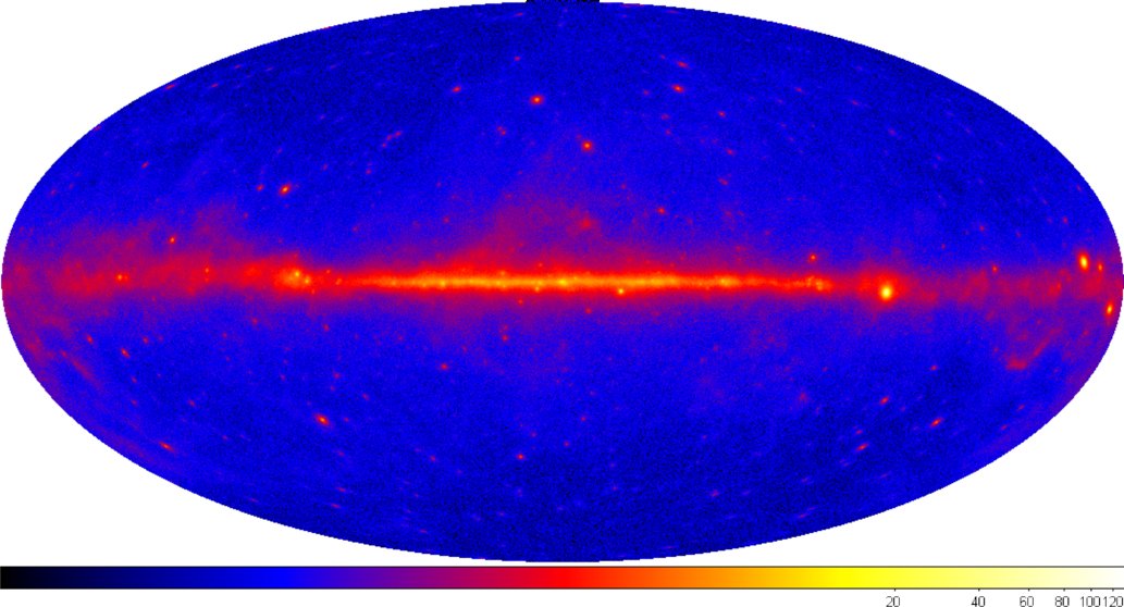
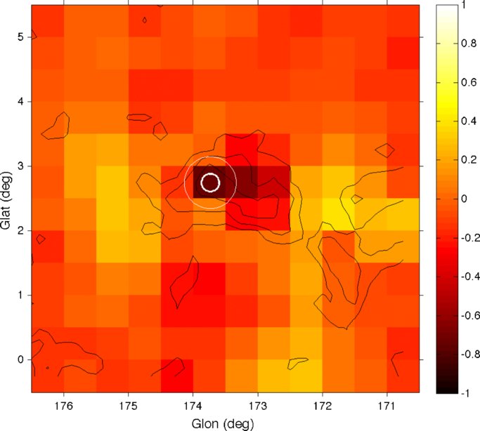