
Abstract
Previous work has shown that PRESAGE® can be used successfully to perform 3D dosimetric measurements of complex radiotherapy treatments. However, measurements near the sample edges are known to be difficult to achieve. This is an issue when the doses at air-material interfaces are of interest, for example when investigating the electron return effect (ERE) present in treatments delivered by magnetic resonance (MR)-linac systems.
To study this effect, a set of 3.5 cm-diameter cylindrical PRESAGE® samples was uniformly irradiated with multiple dose fractions, using either a conventional linac or an MR-linac. The samples were imaged between fractions using an optical-CT, to read out the corresponding accumulated doses. A calibration between TPS-predicted dose and optical-CT pixel value was determined for individual dosimeters as a function of radial distance from the axis of rotation. This data was used to develop a correction that was applied to four additional samples of PRESAGE® of the same formulation, irradiated with 3D-CRT and IMRT treatment plans, to recover significantly improved 3D measurements of dose. An alternative strategy was also tested, in which the outer surface of the sample was physically removed prior to irradiation.
Results show that for the formulation studied here, PRESAGE® samples have a central region that responds uniformly and an edge region of 6–7 mm where there is gradual increase in dosimeter response, rising to an over-response of 24%–36% at the outer boundary. This non-uniform dose response increases in both extent and magnitude over time. Both mitigation strategies investigated were successful. In our four exemplar studies, we show how discrepancies at edges are reduced from 13%–37% of the maximum dose to between 2 and 8%. Quantitative analysis shows that the 3D gamma passing rates rise from 90.4, 69.3, 63.7 and 43.6% to 97.3, 99.9, 96.7 and 98.9% respectively.
Export citation and abstract BibTeX RIS

Original content from this work may be used under the terms of the Creative Commons Attribution 3.0 license. Any further distribution of this work must maintain attribution to the author(s) and the title of the work, journal citation and DOI.
1. Introduction
Advances in engineering and computing in the last 30 years have led to huge improvements in image guidance technology for radiotherapy (RT) treatments. A host of modern radiotherapy techniques, including intensity modulated radiation therapy (IMRT), volumetric modulated arc therapy (VMAT), stereotactic radiotherapy (SRT), proton beam therapy and brachytherapy, give better local tumour control and less dose to normal surrounding tissues, by better conforming the dose distribution to the shape of the target volume. These techniques are both computationally complex to plan and technically demanding to deliver, so experimental validation is essential before treating patients. Although only a few centres currently have the technical expertise to use them, 3D dosimeters have gained popularity over the last decade as a method for dose verification in RT (De Deene and Vandecasteele 2013, Oldham 2015, Khezerloo et al 2017). They are particularly advantageous for end-to-end tests to validate a complete RT treatment chain, as they are nearly tissue equivalent, can be fabricated in different shapes, provide high spatial resolution and record the full 3D dose information (Schreiner 2015).
There are several different classes of 3D dosimeter, with the two most commonly used being polymer gels (Baldock et al 2010), which are read out using either Magnetic Resonance Imaging (MRI), X-ray CT or optical methods, and radiochromic dosimeters(Schreiner 2015), for which optical-CT is the default readout modality (Guo et al 2006). The latter group includes both Fricke gels and a large class of materials all based around leuco-dyes, including surfactant (micelle) gels,plastics and silicone-based dosimeters.
A known issue when using 3D dosimeters is the difficulty of obtaining valid data near the sample edges. Polymer gel dosimeters are sensitive to oxygen so need to be inside a container impermeable to oxygen as glass or barex®, which precludes measurement at dosimeter-air interfaces. Radiochromic plastic samples do not need a container, but do, on the other hand, lead to unreliable readings at the exterior surfaces (Sakhalkar et al 2009, Brady et al 2010, Rehman et al 2015). Until recently, it had been assumed that these were artefacts caused primarily by the optical-CT readout modality and, specifically, a mismatch in refractive index between the matching liquid and the sample (Doran 2013). However, in the last few years, several groups using cylindrical PRESAGE® samples with diameters ranging from 7 to 11 cm have reported edge effects that appear to originate within the samples themselves. (Jackson et al 2015) reported 100% over-response in the 5 mm peripheral region and excluded it from analysis. (Dekker et al 2016) noted a radial increase of sensitivity to radiation, from the centre outwards, leading to an over-response at the edges of between 5% and 20% depending on the sample. (Mein et al 2017) also referred to a radial variation of up to 8% from the centre to the exterior surface, but only when samples were scanned 24 h after irradiation. To date there have been only a few, primarily anecdotal reports on edge effects in micelle, silicone or other types of radiochromic dosimeter.
A plausible explanation for these findings is that the non-uniform sensitivity of the samples is related to processes occurring during manufacture, as a consequence of changes in temperature during curation and/or a loss of solvent from the exterior surface that also continues post-manufacture. This would lead to concentration gradients of some of the reactants involved in the colour-change reaction that is the basis for the quantitative dose measurement. However, no systematic studies of the effect have yet been undertaken. The ad hoc solution of discarding a 5 mm edge from a sample might not be problematic for large diameter dosimeters, but is arbitrary and could represent a considerable loss of information for smaller samples (Teng et al 2014).
In this study, we aim to have a better understanding of the non-uniform sensitivity to radiation (what we call the 'edge effect') of the radiochromic plastic PRESAGE®, by uniformly irradiating samples to successively increasing doses, in order to obtain spatially-resolved dose-response relations that are sample specific. By appropriate normalisation, we demonstrate that useful calibration data can be created allowing us to correct images from other samples fabricated as part of the same formulation. We also investigate an alternative way to eliminate the edge effect by physically removing a thin layer of material from the sample surfaces.
Finally, we choose exemplar case studies in the areas of small-field dosimetry and the electron return effect (ERE) to test the quality of the correction. The technique is widely applicable and we believe that the results will also be relevant to many other areas, including brachytherapy, phantoms mimicking inhomogeneous tissues (particularly the simulation of treatments to lung tumours), and any type of experiment requiring small 3D dosimeter inserts in anthropomorphic phantoms.
2. Material and methods
2.1. PRESAGE® samples
A large number of samples from a single formulation of PRESAGE® was ordered from the manufacturer (Heuris Pharma, Skillman, NJ, USA) and used to study consistency between samples, potential magnetic field effects during irradiation, and both spatial and temporal variations in dose response. Further samples from the same order were used to demonstrate a correction methodology. Table 1 summarises the different samples used in this work, with information regarding the irradiated doses, the time between manufacture and irradiation in months and the purpose of their use.
Table 1. Summary of the irradiated samples used in this study, from a single PRESAGE® formulation, containing information regarding time between manufacture and irradiation, doses and the purposes for which samples were used in this work.
| Sample | Interval between manufacture and irradiation/months | Dose/Gy | Purpose |
|---|---|---|---|
| a1, a2 | 1.7 | 0, 2, 4, 6, 8, 10 | Uniform irradiation in conventional linac (B = 0) to obtain calibration (2.3.1) |
| a3, a4, a5 | 4.3 | 0, 2, 6, 10 | |
| a6 | 8.8 | 0, 2, 6, 10 | |
| a7plan | 2.4 | max 9.7 | Exemplar studies demonstrating correction process using a standard linac (2.5) |
| a8plan | 7.1 | ||
| a9 | 4.3 | 0, 6, 12 | Uniform irradiation with physical modification of sample and measurement at the edges (2.6) |
| a10 | 4.3 | ||
| a11MRL | 9.6 | 0, 5, 10 | Uniform irradiation in MR-linac (B = 1.5T) to obtain calibration (2.3.2) |
| a12planMRL | 9.6 | max 13.2 (ERE) | Exemplar studies as above, but with irradiation in MR-linac (2.5) |
| a13planMRL | max 8.0 |
PRESAGE® samples were manufactured using silicone moulds to create cylinders of diameter 3.5 cm ranging in length from 5.3 cm to 5.9 cm depending on the degree to which the moulds were filled. Each sample had a flat base and a curved meniscus. After approximately a week in transit at ambient temperature, samples were stored in the dark in a fridge for the duration of the study. Each sample was glued to a 3D-printed plastic cap that was used to position the samples in a reproducible way during imaging (figure 1) and irradiation (figures 2(a) and (b)).
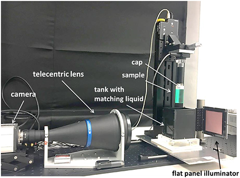
Figure 1. In house telecentric optical-CT scanner used in this work. The vertical stage is used to lower the sample and place it inside the matching liquid. The hardware is controled by in-house developed LabView® code.
Download figure:
Standard image High-resolution image
Figure 2. (a) Small sample of PRESAGE® attached to the in-house holder created to place it inside (b) the QUASARTM MRI4D phantom in a reproducible position. (c) Sample a9cut reduced in diameter. CT scan of the phantom with a dummy PRESAGE® sample showing the dose distribution calculated by (d) 3D-CRT and (e) IMRT planning, and delivered to sample a7plan and a8plan respectively.
Download figure:
Standard image High-resolution image2.2. Optical-CT imaging
The in-house optical-CT scanner that was used to measure differences in optical density (OD) within a 3D sample is pictured in figure 1. The system consists of a camera (Zyla sCMOS, Andor Technology PLC, Belfast, UK) connected to a telecentric lens (TC2MHR096-C, 0.137x magnification, Opto-Engineering, Italy) which allows a maximum field of view (FOV) of 121.17 × 102.2 mm, a flat panel illuminator (PHLOX-LEDR-BL-100 × 100-S-Q-IR-24 V, PHLOX, Aix-en-Provence, France) and a rotation stage (CR1/M-Z7 K, Thorlabs Ltd, Ely, UK). To perform a scan each sample was placed between the lens and the illuminator and inside a matching tank, filled with a mixture of 2-ethylhexylsalicylate and 4-methoxycinnamicacid 2-ethylhexylester, whose refractive index was adjusted to be a good match to that of the PRESAGE® samples (Abdul Rahman et al 2011). Scanning procedures followed the guidelines in (Doran 2013), with samples removed from the fridge 90 min prior to positioning in the scanner, followed by a further 5–10 min. period for the matching liquid to 'settle' before scanning. 1000 projections were obtained over a 180° rotation and reconstructed using filtered back projection at a high native resolution of (0.24 mm × 0.24 mm × 0.19 mm) before being re-sampled to a more clinically relevant resolution (0.5 mm × 0.5 mm × 0.5 mm) for comparison with the treatment planning system.
2.3. Investigation of the spatially non-uniform response of PRESAGE®
2.3.1. Reproducibility and time-dependence for a single formulation
Samples were irradiated at three different time points after their manufacture: 1.7 months (a1, a2), 4.3 months (a3, a4 and a5) and 8.8 months (a6). Samples a1 and a2 were irradiated uniformly in steps of 2 Gy, receiving accumulated doses of 2, 4, 6, 8 and 10 Gy. The relation between dose and optical-CT pixel value was expected to be linear, a result observed in the vast majority of previous literature for PRESAGE® when used within the routine clinical dose range (Guo et al 2006, Jackson et al 2015). Thus, after verification using samples a1 and a2, the remainder of samples a3 to a6 received only three accumulated dose levels: 2, 6 and 10 Gy.
The samples were irradiated using a conventional linac (Synergy, Elekta AB, Stockholm, Sweden), and placed inside an MP1 water tank (PTW, Germany) at 90 cm source-to-surface distance (SSD) and 10 cm depth. To deliver a uniform dose, each sample was irradiated with four 6 MV beams and field size 10 × 10 cm2. The gantry was always kept at 0° with samples rotated by 90° between beam deliveries. With this set-up, dose uniformity within a sample of PRESAGE® is expected to be within 0.1% as given by Raystation (RaySearch Medical Laboratories AB, Stockholm, Sweden) treatment planning system (TPS) dose calculation. A sample holder allow the sample to be placed completely parallel to the beam axis so no changes in dose transverse to the sample are expected.
Each sample was imaged 1–3 h before the first irradiation ('pre-scan') and subsequently at a constant 1 h after each irradiation ('post-scan') to control for changes in the dose response that might be related to post-irradiation time (Mein et al 2017).
2.3.2. Magnetic field dependence
A further sample a11MRL was irradiated in an MR-linac (Elekta Unity, AB, Stockholm, Sweden) with accumulated uniform doses of 5 Gy and 10 Gy. The Elekta MR-linac system comprises a 1.5T Philips magnet and a 7 MV Linac. The same MP1 water tank was used and the conditions applied in section 2.3.1 were adapted here. Because of the MR-linac bore size of 70 cm in diameter and the fixed table height, the samples were positioned 10 cm away from the lateral side of the tank and the gantry at 90°, at the isocentre with SSD = 143.5 cm.
2.4. Correcting the spatial non-uniformity of dose response
Exploiting the cylindrical symmetry of the samples and the linearity of the bulk material dose- response, we hypothesise a spatially non-uniform dose response as follows:

where  , with
  , corresponds to the change in optical-CT value between the pre- and post- scans for a voxel with in-plane coordinates
  , after irradiation to an accumulated dose
  .
.  is the gradient of the dose-response for points at a distance
  from the axis of rotation of the sample, and
  is the intercept of the fit line, which should be zero. A diagram of the steps described in this section, performed to obtain a calibration image to correct for PRESAGE® samples non-uniform response, can be found in figure 3.
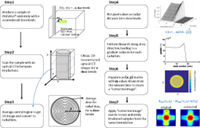
Figure 3. Diagram displaying the steps required to obtain a calibration image to correct for the non-uniform dose response of PRESAGE® samples.
Download figure:
Standard image High-resolution imageTo improve the signal-to-noise ratio the calibration is obtained via longitudinal and radial averaging.
First, input 3D images of the uniformly irradiated cylinders are averaged longitudinally. As shown later, the edge effect extends inwards from each surface by 6–7 mm. Therefore, in order to avoid any end effects, we average source data from only the axial slices occupying the central 2.9 cm of the sample, yielding a 2D mean-image for each accumulated dose.
Next,  is discretised and image pixels
  are assigned to radial bins
  , corresponding to annuli of width
  , such that

Pixels in each annulus are averaged for each accumulated dose level and the mean values fitted to a straight line (i.e. a 6-point fit for samples a1, a2; a 4-point fit for a3–a6; and a 3-point fit for a11MRL). This gives a single value of  for each bin, where
  is the bin centre. The intercept
  is close to zero everywhere (ranged from 10–5 to 10–6) and can henceforth be ignored.
The resulting calibration is then applied to the measurement of a test dose distribution on a different sample from the same formulation using the following equation:

where  is the centre of the bin containing
  . In practice, we simply compute a 'correction image' by populating an
  matrix with
  values drawn from the relevant bins. The correction is then applied to the 3D images by dividing each axial slice of the source data by the 2D correction image. Note that we did not attempt to model or correct data in the longitudinal direction, because of the complexities introduced by the curved meniscus and inconsistent length of samples supplied by the manufacturer.
2.5. Validation of sample correction
As shown in figure 2, sample a7plan was mounted in the central cylinder of a QUASARTM MRI4D phantom (Modus Medical Devices Inc., London, Ontario) and irradiated with a 3D conformal radiotherapy plan consisting of four equidistant 6 MV beams of field size 3 cm × 1.5 cm, to a maximum dose of 9.7 Gy (figure 2(d)). The top and bottom edges of the samples were trimmed with a saw and finished with a lathe to keep a consistent 5 cm length in all samples.
Two additional samples were irradiated with a more clinically representative dose distribution: an IMRT plan with 5 beams (figure 2(e)). Sample a8plan was irradiated on a conventional linac, while sample a13planMRL was irradiated in the MR-linac. Sample a12planMRL was also irradiated in the MR-linac, but with a single beam (gantry at 0°), and field size of 3 cm × 5 cm, in order to observe a dose enhancement at the detector edge due to the ERE.
All treatment plans were calculated on a CT scan of a dummy PRESAGE® sample of identical dimensions placed in the QUASAR™ MRI4D phantom. For the plans delivered on the standard linac, research version of Monaco 5.19.03 (Elekta AB, Stockholm, Sweden) was used as the TPS, while for the plans delivered at the MR-linac, a clinical version of Monaco 5.4 was used instead. All simulations were performed with isotropic (1 mm)3 voxel size and 1% uncertainty of dose-to-medium. Both PRESAGE® reconstructed images and Monaco calculated dose distributions were normalized to the region of maximum dose and rescaled to an isotropic voxel size of (0.5 mm)3 before being registered with each other. The correction images obtained from uniformly irradiated samples were applied to data from the non-uniformly irradiated samples and agreement between the experimental measurements and TPS calculations was investigated by applying a local 3D gamma (Depuydt et al 2002) criterion of either 3%/ 2 mm or 2%/ 2 mm, with a 10% threshold.
Gafchromic EBT3 films with the same length and width as PRESAGE® samples (5 cm × 3.5 cm) were sandwiched between two Perspex half cylinders with the same dimensions as the PRESAGE® samples and irradiated in the same conditions. We irradiated films in a few planes for comparison with PRESAGE® (samples a7plan, a8plan and a13planMRL) and TPS simulations. Films were scanned in transmission mode, with 48bit RGB and 150dpi.
The films from the batch used in this study had been previously calibrated on the MR-linac and also on a conventional linac. To do this rectangular pieces of film were placed in between slabs of a solid water phantom (type RW3 PTW-Freiburg, Germany), at 10 cm depth and at the system isocentre. For each calibration curve, 6 films were used and irradiated with doses from 0 to 16 Gy. FilmQA Pro software (Ashland, NJ, USA) was used to obtain a calibration curve based on the multichannel film dosimeter approach (Micke et al 2011). Film analysis was carried out using the same software in order to convert the pixel values to dose.
2.6. Physical removal of sample surface layer
As most of the non-uniformities in the samples occur near the surface, an alternative to applying a correction could be the physical removal of an outer layer from the samples. In a previous study, we showed preliminary evidence that cutting samples of PRESAGE® eliminates the non-uniform response of PRESAGE® at the edges (Costa et al 2018). Here, in two exemplar experiments, we physically modify samples to investigate how suitable this approach is for mitigation of the non-uniform dose response and the measurement of surface doses.
Both samples a9 and a10 were irradiated uniformly in their original states with 6 Gy and scanned after 1 h. Sample a9 was then reduced in diameter by 1 cm using a lathe. Sample a10 was altered by drilling a 1 cm core to demonstrate how dosimetry can successfully be performed immediately adjacent to internal cavities. They were immediately rescanned and then once again uniformly irradiated with an additional 6 Gy, before a final scan was performed after 1 h.
3. Results
3.1. Sample uniformity characterization
3.1.1. Reproducibility and time-dependence
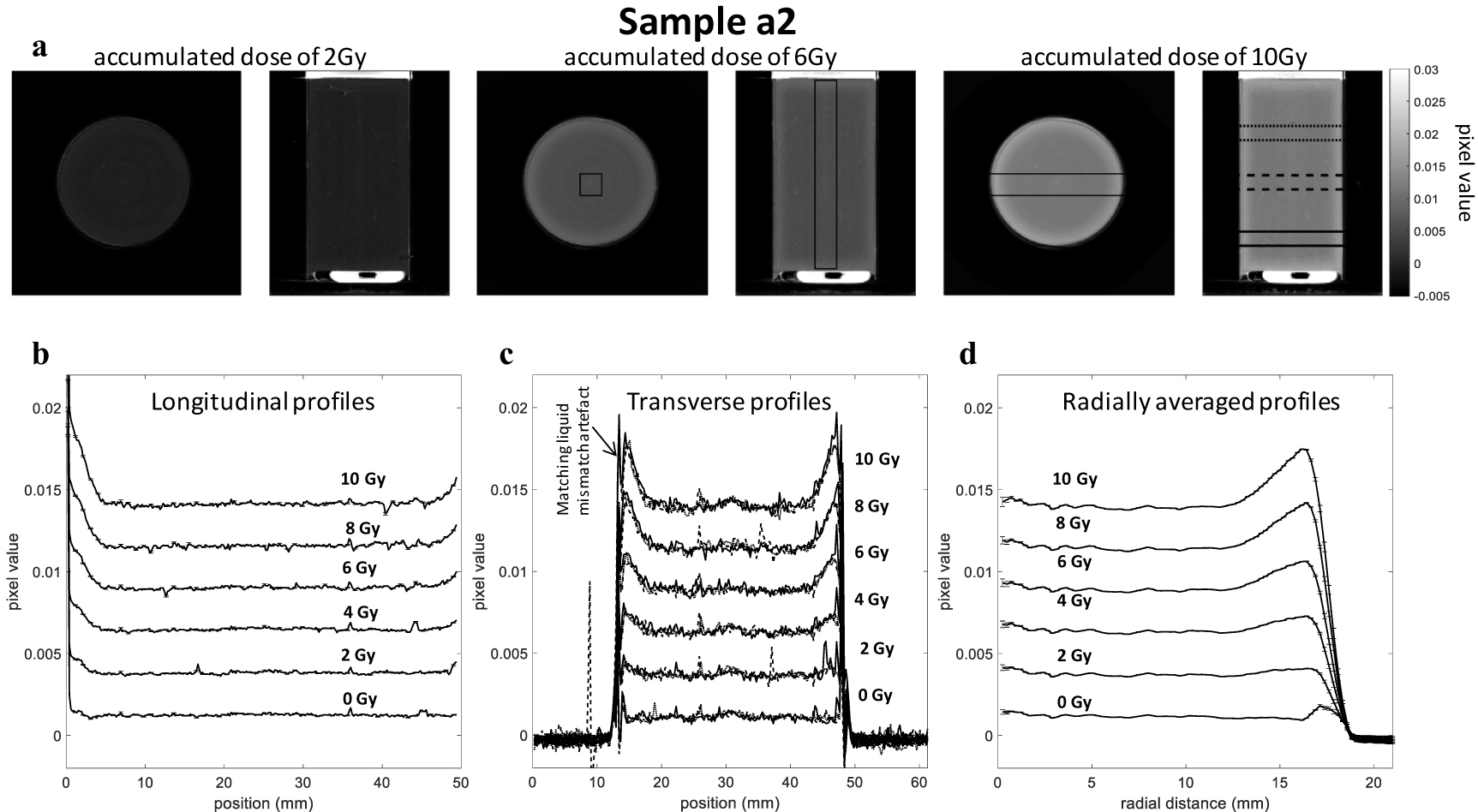
In figure 4, an increased optical-CT pixel value is observed over the outer 6–7 mm of sample a2, both at the top and bottom edges and around the rim. This enhanced colour change demonstrates a spatially non-uniform response of the PRESAGE® to radiation. For samples a1 to a5, the difference between the dose sensitivity between the centre and the edges, ranged from 24% to 36%. The absolute differences in pixel value become smaller for lower accumulated doses, suggesting strongly that this is not an optical artefact resulting from the CT scanning process. By contrast, a known optical edge artefact, caused by residual refractive index mismatch, is visible in figure 4(c), with a much smaller extent into the sample (0.5–1.4 mm for samples a1 to a5). Figure 4(a) shows that, at any given radial coordinate, the relation between absorbed dose and PRESAGE® radiochromic response is linear. However, near the dosimeter edges, the slope of the fit lines (given by the gradient m in equation (1)) increases, indicating enhanced dose sensitivity.
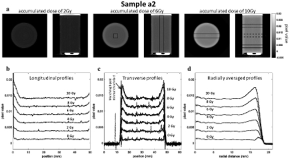
Figure 4. (a) 2D transverse and longitudinal slices of the reconstructed optical-CT image for sample a2 with accumulated dose of 2 Gy, 6 Gy and 10 Gy, showing a visible edge effect. (b) Transverse profiles were obtained by averaging over the 4 mm × 4 mm cross-sectional area of a cuboidal column along the length of the sample as indicated on the 6 Gy images. The error bars represent one standard error of the mean. The profiles show the results for the pre-scan and five accumulated dose levels (c) Transverse profiles were taken at different positions along the sample length, which are drawn on the 10 Gy images. For each dose level the plots are overlaid to show the small variation along the sample length. (d) Sample a2 radial average for each accumulated dose obtained by averaging the axial slices in the central region of the sample (constituting 2.9 cm of the sample). Error bars represent one standard error of the mean of each radial distance.
Download figure:
Standard image High-resolution imageFigure 5(b) demonstrates different absolute dose sensitivity values in the central region of up to 38% between samples from the same dosimeter formulation. These results were discussed with the manufacturer, who explained that the single order had been fulfilled in the form of two nominally identical batches manufactured on different days, but that these had not been segregated when packed. Based on the grouping of the profiles in figure 5(b), we surmise that samples a1, a4 and a3 were likely to have come from the same batch, with samples a2 and a5 from the second batch. However, it was beyond the scope of the current study to characterise batch-related effects exhaustively.
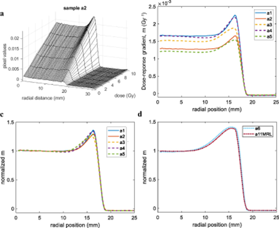
Figure 5. (a) Relationship between optical-CT pixel value and dose for the sample a2 as a function of radial distance. (b) Gradient of dose-response (m) versus radial position for samples a1 to a5, demonstrating both a variation in sensitivity of each sample in the radial direction and a variation in the absolute value of the sensitivity between samples. (c) Radial plots of m values, normalised to 1 at the centre of the samples show a broadly similar pattern of relative sensitivity as a function of radial position for samples a1 to a5. (d) Radial plots of normalised m values for samples a6 and a11MRL, which were irradiated significantly later show a much more extensive edge effect.
Download figure:
Standard image High-resolution imageRather, we focus here on the mitigation of any such effect. Figure 5(c) demonstrates that, regardless of absolute response, all samples from this formulation had very similar spatial variations in relative sensitivity (normalised m value) with accumulated dose. All samples displayed a uniform dose response in the central volume with an increase in sensitivity at the outer edges, the extent of which depended on their age by the time they were irradiated. A quantitative measure for their similarity is found by taking the root mean square (rms) difference between the profiles of figure 5(c) over the region of the edge effect (radial position 11–17 mm). The rms difference between the profiles a1 and a2 is 2.9%, while the mean rms between the profiles a3, a4 and a5 is 3.9%. The mean rms considering all samples a1–a5 is 4%. More information on the edge difference over time can be found in appendix B.
Comparison of figures 5(c) and (d) shows a clear increase in the extent of the edge effect over time that from around 6 to 7 mm in 2.6 month and to approximately 13 mm after 7.1 months. An increase of the magnitude of the effect (∼40% increase in dose sensitivity at the edges for sample a6 and a11MRL, compared to a 24%–36% increase for the other samples).
Further data (not shown) confirm that only one dose point plus the pre-scan is necessary to calibrate the correction: the radial average  is almost identical when calculated using only the pre-scan and a 6 or 10 Gy image, compared with the result of a linear fit to data from multiple images. However, using only the data from the pre-scan and 2 Gy image was insufficient for obtaining a satisfactory calibration.
3.1.2. Magnetic field dependency
The radial dose-response of two samples irradiated within a month, one at the research linac (sample a6) and the other at the MR-linac (sample a11MRL), are very similar after normalization (figure 5(d)). The rms difference between the two profiles of figure 5(d) over the region of radial position 9–17 mm is 3.1%, which is within what was observed for the other samples a1–a5. These results support previous data (Costa et al 2018, Lee et al 2017), which showed that PRESAGE® samples were not affected by a constant magnetic field.
3.2. Performance of the correction procedure
If no correction is applied, PRESAGE® measurements of non-uniform irradiations disagree markedly with planning system predictions in the outer 6–7 mm of the sample (figures 6–8). For samples a7plan, a8plan, a12planMRL and a13planMRL, the maximal errors in the profiles shown here were approximately 23%, 13%, 37% and 35%, respectively, of the maximum dose. Use of the correction methodology described above improved results dramatically. By applying the best correction image, high relative dose differences could be reduced to a maximal error that varied between 2 and 8% and was less than 5% of the maximum dose for the majority of the corrected region. The corresponding 3D gamma passing rates (2%/2 mm with a 10% threshold) improved from 90.4%, 69.3%, 63.7% and 43.6% for uncorrected images to 97.3%, 99.9%, 96.7% and 98.9%, respectively, when the best performing correction was applied (see table 2).
Table 2. 3D Gamma passing rates for the comparison of experimental data for PRESAGE® and Monaco simulations. For each of samples a7plan, a8plan, a12planMRL and a13planMRL, we show results using two different gamma criteria (each with a 10% threshold), both without correction and with correction using data from a number of different calibration samples. The table line with the highest gamma passing rate for each sample is shown in bold.
| Irradiation | Sample providing the correction data | Irradiation time mismatch (months) | 3%, mm | 2%, 2mm |
|---|---|---|---|---|
| a7plan | no corr | – | 97.3 | 90.4 |
| a1 | −0.7 | 99.6 | 96.4 | |
| a2 | 99.4 | 95.4 | ||
| a3 | 1.9 | 99.2 | 96.4 | |
| a4 | 99.6 | 97.3 | ||
| a5 | 99.5 | 97.1 | ||
| a6 | 6.4 | 98.4 | 92.2 | |
| a8plan | no corr | – | 85.2 | 69.3 |
| a1 | −5.4 | 100.0 | 97.2 | |
| a2 | 100.0 | 97.0 | ||
| a3 | −2.8 | 99.6 | 98.8 | |
| a4 | 100.0 | 98.9 | ||
| a5 | 100.0 | 99.7 | ||
| a6 | 1.7 | 100.0 | 99.9 | |
| a12planMRL | no corr | – | 66.7 | 63.7 |
| a11MRL | 0 | 97.8 | 96.7 | |
| a6 | −0.8 | 97.7 | 96.4 | |
| a1 | −7.9 | 81.3 | 78.4 | |
| a13planMRL | no corr | – | 45.3 | 43.6 |
| a11MRL | 0 | 99.0 | 98.6 | |
| a6 | −0.8 | 99.3 | 98.9 | |
| a1 | −7.9 | 70.6 | 68.2 |

Figure 6. Comparison of normalized 2D axial and longitudinal dose distributions, without correction and after applying correction images based on data from six different calibration samples, for sample a7planirradiated on the conventional linac. For each of the left-right (LR), anterior-posterior (AP), diagonal and longitudinal profiles we plot the measured data and the Monaco TPS output together in the upper panel, and then the difference between measurement and TPS for each set of calibration data in the lower panel. Longitudinal profiles corrected by different images (a1–16) overlap as they are taken through the centre of the sample, where no correction is needed (i.e. the correction is applied but the correction factor is 1). EBT3 films normalized profiles and respective differences when compared with Monaco calculated data are shown for LR, AP and longitudinal profiles. Note that the suitability of the correction image used depends on the time it was obtained. For example, sample a6 was obtained 6.4 months after sample a7plan was irradiated and thus overcorrects it (see table 2). Profiles corresponding to the correction image that led to the highest gamma passing rate (displayed in bold in table 2) are highlighted by plotting a thicker line.
Download figure:
Standard image High-resolution imageWe explored the effect of applying corrections based on calibration data obtained from each of samples a1–a6. In our studies, correction always improved the results, but performed best when there was a good match between the sensitivity profiles of the calibration and measurement samples. This meant that the time evolution of the samples, as illustrated in figures 4(c) and (d), was important. The data of table 2 show that, for all four exemplars, the worst performance of the correction algorithm occurs when the calibration data are derived from the sample with largest mismatch in irradiation time from that of the test sample. Films displayed a good agreement with both PRESAGE® and Monaco calculations, showing a relative dose difference similar to what was obtained with PRESAGE® (see figures 6 and 7) with difference in relative doses below 5% for the majority of the measured values.
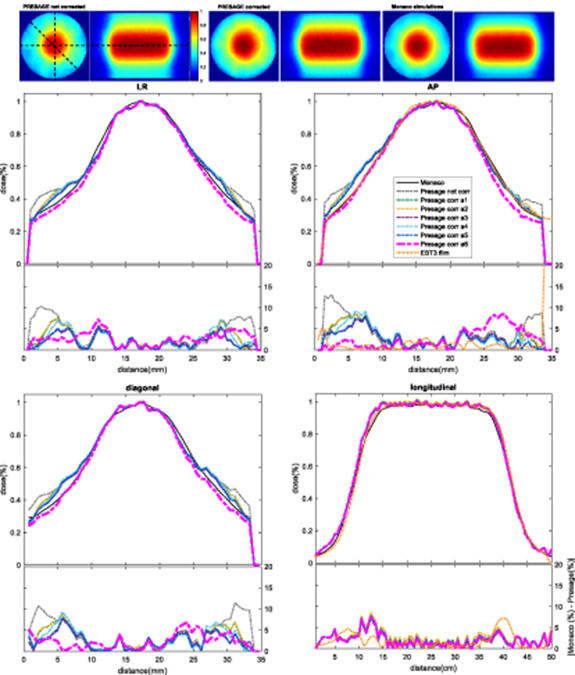
Figure 7. Comparison of normalized 2D axial and longitudinal dose distributions, without correction and after applying correction images based on data from six different calibration samples, for sample a8plan on the conventional linac. For each of the left-right (LR), anterior-posterior (AP), diagonal and longitudinal profiles we plot the measured data and the Monaco TPS output together in the upper panel, and then the difference between measurement and TPS for each set of calibration data in the lower panel. Longitudinal profiles corrected by different images (a1–16) overlap as they are taken through the centre of the sample, where no correction is needed (i.e. the correction is applied but the correction factor is 1). EBT3 films normalized profiles and respective differences when compared with Monaco calculated data were also obtained for AP and longitudinal profiles. Profiles corresponding to the correction image that led to the highest gamma passing rate (dis played in bold in table 2) are highlighted by plotting a thicker line.
Download figure:
Standard image High-resolution image3.3. Physical removal of sample surface layer
Figure 9 shows that the edge effect disappears in the regions where material is physically removed from sample a9, again suggesting strongly that the effect is not an artefact of the optical scanning. The non-reappearance of the effect after the sample was irradiated with an additional 6 Gy shows that newly exposed surfaces do not immediately acquire an enhanced sensitivity, although additional results suggest that the effect can reappear if samples are irradiated after a delay of a month (see supporting data in appendix B, figure B2).
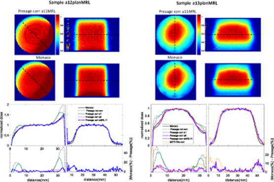
Figure 8. Comparison of normalized 2D axial and longitudinal dose distributions, without correction and after applying correction images based on data from three different calibration samples, for the two exemplars irradiated on the MR linac. The longitudinal view is rotated by 90° to be representative of the sample position during irradiation. Plotted profiles show additional applied correction images and respective difference between Monaco TPS and PRESAGE® (or film) normalized profiles. Both samples reconstructed images show noisy data as a consequence of the samples age. The artefact visible on the longitudinal 2D image of sample 12planMRL corresponds to the end of the sample and was removed in the profile. Note that the quality of the correction image used depends on the time it was obtained. Sample a1 was obtain 7.9 months before sample a12planMRL and a13planMRL were irradiated, under-correcting it (see table 2). The profiles corresponding to correction image that led to the highest gamma passing rate are highlighted by plotting a thicker line.
Download figure:
Standard image High-resolution image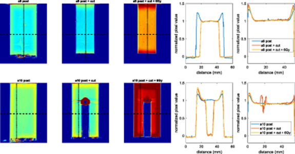
Figure 9. Central longitudinal view of sample a9 and a10 reconstructed images before and after being physically changed and uniformly irradiated with additional 6 Gy. Air bubbles are present in both bottom of the samples and inside the hole in sample a9cut, causing obvious but not troublesome image artefacts. Dose distribution images are shown in absolute values to distinguish between different accumulated dose levels, whereas profiles are shown after normalization to the flat region of each reconstructed image to highlight the high degree of agreement. Longitudinal profiles are averaged over the middle of the samples. For sample a10, this corresponds to the available region without the hole. Transverse and longitudinal profiles were averaged over 20 pixels (∼5 mm) in both directions.
Download figure:
Standard image High-resolution imageFor both samples a9 and a10, the additional irradiation does not change the spatial distribution of relative dose and this explains why the orange curve overlays the red one so precisely as the normalized pixel value are within <1.5% for sample a9 scanned at all different stages (as well as providing confirmation of the reproducibility of our optical-CT scanning methods).
Sample a10 shows that it is possible to drill a hole in the sample and still obtain valid data near the internal edges. As long as irradiation and imaging take place soon after the sample is modified, there is no need to apply a correction for the edges that were removed or drilled, as the central region of the sample has uniform response to dose. Note how the edge effects seen on images of both samples are still visible for regions that were left in their original state.
4. Discussion
In this study, we developed a methodology to correct the over-response of PRESAGE® to dose at sample edges, based on images obtained by uniformly irradiating calibration samples. This correction allows us to obtain information about the dose distribution delivered to small samples of PRESAGE® that it would not otherwise be possible to obtain. We did not attempt to apply a correction image that would account for absolute changes in sensitivity but rather to correct relative sensitivity changes as a function of radius.
4.1. Time, magnetic field, intra and inter-formulation dependency
Results shown in figures 4 and 5 illustrate that samples have a central region where there is an approximately uniform response to dose and an outer 'skin' of ∼6–7 mm, or ∼13 mm, where the sensitivity to dose can increase by up to 24%–40% depending on the sample and its age. The extent of this region changes over time, as shown in figures 5(c) and (d), where samples a6 and a11MRL were irradiated 7–8 months after samples a1 and a2 (figure B1). The small difference between sample a6 and a11MRL after normalization provides anecdotal evidence that irradiation in a conventional linac or in the MR-linac does not influence the spatial distribution of the PRESAGE® dose response. However, samples of the same formulation can have markedly different absolute sensitivities. This we regard as an almost inevitable consequence of chemically-based dosimetry using materials incorporating long-chain polymers, and is something that is very familiar in traditional polymer gel dosimetry (Vandecasteele and De Deene 2012).
As detailed in the appendix A, additional studies not reported as part of the main text, show that changing the percentage of solvent in the PRESAGE® formulation leads to observable changes in the spatial variation of sensitivity.
Applying any of the correction images to non-uniformly irradiated samples (figures 6–8) improves the agreement between the measured data and the prediction from the TPS. This is clear by looking at both profiles and 3D gamma passing rates (table 2). For sample a11MRL, these results show how the correction completely transforms our ability to measure near the edges, and in this case allows us to make 3D measurements of the ERE that could not currently be obtained by any other non-imaging method (figure 8). The images here have higher spatial resolution and better signal-to-noise than the equivalent MRI-based dosimetry data recently published by (Mcdonald et al 2018), but the PRESAGE® material cannot mimic low density regions.
As expected, and as a consequence of a presumed chemical change leading to an extension of the edge effect over time, all non-uniformly irradiated samples show better agreement with TPS simulations when corrected using calibration data from samples uniformly irradiated at a matching time point.
4.2. Physical removal of sample surface layer
The calibration and correction methodology demonstrated here reduces the dose measurement error at the sample edges to a clinically acceptable level. Nevertheless, it is of interest to try and eliminate errors at source, and the physical removal of the outer edges of the samples prior to irradiation completely mitigates the edge effect on these samples. Although it might be difficult to integrate with a clinical workflow, this is good alternative to applying a correction, provided that a sample is ordered with dimensions larger than those needed for the eventual measurement, and assuming that workshop facilities are available for cutting the sample with high accuracy. None of the scan results showed any evidence that the act of machining the samples caused changes to the dose-response characteristics of the adjacent PRESAGE® left behind, which is an encouraging finding.
4.3. Sources of edge effects
It is important to realise that edge effects in optical-CT can arise in different ways: (1) a genuine change in the PRESAGE® sensitivity to radiation, which is the main focus of this paper; (2) the well-known artefact caused by a mismatch between the matching liquid and the samples; (3) an artefact previously observed for highly light-absorbing samples (Al-Nowais and Doran 2009) which leads to reconstructed images with a lower intensity in the middle than the edges; (4) effects attributed to scattering, as reported by (Bosi et al 2009).
The physicochemical origins of the observed effects, which have been seen by others before (Dekker et al 2016, Mein et al 2017), have been discussed with the manufacturer. Our current working hypothesis is that, both during the curing process and subsequently over time, solvent is lost from the sample at exposed surfaces, thus altering the chemistry that occurs when the samples are irradiated. It is plausible that this effect could be ameliorated via changes in the preparation procedure for the samples, but further work is needed in this area.
The artefact mentioned in (2) is also visible in our samples but, typically, affects a millimetre or less around the edges. We expect this artefact to be difficult to eliminate, because, in practice, it is not possible to obtain a perfect refractive index agreement between the sample and the matching liquid, particularly if there are temperature variations in scanning conditions.
As described in the appendix, there are tentative indications that some of our results for other formulations may also have been affected by artefacts of type (3). However, more work would be needed to confirm this.
We do not expect PRESAGE® samples to suffer from issue (4), as the origin of its optical contrast is absorption, not scattering.
4.4. Practical guidelines
Based on the studies above, the following recommendations may be made if performing measurements using PRESAGE®, particularly if interested in accurately measuring dose at the sample edges:
- (a)Order or manufacture a batch with enough samples to use one (or more) as uniformly-irradiated calibration samples (section 2.3.1) to obtain a correction image, with the remaining 'test samples' used for the experiments of interest. All samples should have the same diameter and should be similar in length.
- (b)Where possible, irradiate any calibration sample at the same time as the test samples to reduce changes in the samples' sensitivity over time.
- (c)If this is the first time irradiating a batch or specific formulation, make sure artefacts caused by extremely high absorption are not present for higher doses, by testing linearity with dose using several samples.
- (d)Assuming linearity, obtain the calibration data by pre-scanning the selected sample and then irradiating it uniformly, and then scanning the sample one hour after irradiation. We suggest using a higher dose than the maximum dose to be delivered to the test samples, to cover the full range of measurements with good signal-to-noise ratio.
- (e)For each scanned and reconstructed image, exclude the top and bottom edge of the sample, and average the central slices along the sample length where there is a small variation between axial slices.
- (f)Apply the correction image slice by slice to the irradiated test sample using equation (3). The 6–7 mm top and bottom edges of the test sample should not be considered, as the correction would not be accurate for those regions.
- (g)If one expects to irradiate samples for a period longer than 3 months, we recommend saving a sample to uniformly irradiate at a later time point, in order to identify possible changes over time and possibly interpolate the correction images.
- (h)We suggest that, for cylindrical samples with a meniscus, it is likely to be easier to trim the two ends of the sample to mitigate the end effect, rather than attempt to model it.
5. Conclusion
In this study, we have shown that samples of PRESAGE® have increased sensitivity to radiation at their edges, and that the physical size and magnitude of this effect depends on the sample formulation and its age. We successfully improved the measured dose distribution of non-uniformly irradiated samples by applying a correction image obtained from uniformly irradiated calibration samples of the same formulation. Both plans delivered by a conventional linac and by an MR-linac showed better profile agreement with simulations and higher 3D passing rates after correction, with relative dose errors at the sample surface being improved from up to 37% to 2–8%. As an alternative, and when samples allow, we suggest physically removing the edges of the sample to perform measurements near the edges, provided that bigger samples are obtained and that the samples have a central region where a uniform response to dose exists.
A better understanding of the factors influencing PRESAGE® sensitivity is needed before a correction image can be applied to absolute rather than relative values of dose. Nevertheless, the results from this work make it possible for the first time to exploit the full volume of small PRESAGE® samples and to have confidence in the results on the exterior margin of the samples. This could have important implications not only in the field of MR guided radiotherapy, where changes in the dose distributions are expected to occur near tissue-air interfaces, but also to validate treatments such as stereotactic radiotherapy in the lung, where measurements near the dosimeter-air interface are needed.
Acknowledgments
SJD acknowledges receipt of CRUK and EPSRC support to the Cancer Imaging Centre at ICR and RMH in association with MRC and Department of Health C1060/A10334, C1060/A16464 and the NHS funding to the NIHR Biomedical Research Centre and the Clinical Research Facility in Imaging. The Institute of Cancer Research is supported by Cancer Research UK under Programme C33589/A19727.
Appendix A.: Results for alternative PRESAGE® formulations
Using the methods in the main text, the non-uniform dose response was also investigated for three additional batches of PRESAGE®, each with different percentages of solvent content. Denoting the formulation used in the main body of the paper as Formulation a, these new batches were Formulations b, c, and d. A higher solvent content was expected to have effects on dose sensitivity, response stability over time and spatial uniformity of the dose-response.
Table A1 gives the composition of the different formulations, whilst table A2 lists the samples measured.
Table A1. Composition of formulations a, b, c and d investigated in the study.
| Formulation a | Formulation b, c and d | |
|---|---|---|
| Solvent name(s) and wt/wt % | 2% DCM/1% Toluene | 10%, 15%, 20% Dimethylphthalate |
| Leucodye | 1% 2-methyl LMG-DEA | 1% 2,4 dimethyl LMG-DMA |
| Initiator | 0.4% CBr4 | 0.4% CBr4 |
| Polyurethane | BJB–782 | BJB–782 |
| Diameter dosimeters | 3.5 cm | 3.5 cm |
Table A2. Details of the further samples irradiated manufactured with different formulations.
| Formulation (solvent %) | Sample | Interval between manufacture and irradiation (months) | Dose (Gy) | Purpose |
|---|---|---|---|---|
| b (10%) | b1, c1, d1 | 0.7 | 0, 2, 6, 10 | Uniform irradiation to obtain correction image |
| c (15%) | b2plan, c2plan, d2plan | 0.7 | max 9.7 | Application of correction |
| d (20%) | b3MRL, c3MRL, d3MRL | 1.4 | 0, 5, 10 | As above but in the MR-linac |
| b4MRL, c4MRL, d4MRL | 2.9 | 0, 2, 6, 10 |
The main findings of the additional study are as follows:
- Formulations b, c and d demonstrated a different pattern of sensitivity, in which there was not a uniform central region with well-defined edge, but rather a gradual variation in intensity from the centre to the edge (figure A1(a)).
- Normalised radial profiles from different formulations did not overlap over the outer ∼6 mm of the sample (figure A1(b)).
- The dose response for these three formulations displayed non-linearities (figure A1(c)), something which is uncharacteristic for PRESAGE®. This effect was more evident for samples irradiated at a later time point. It was beyond the scope of this work to study this effect in detail. This non-linearity means that correcting data on the basis of a single calibration image could be unsound. Nevertheless, for all the samples measured, our correction method improved the gamma passing rates.
- Formulations b, c and d darkened noticeably with time (figure A1(d)). This is important, because it reduces the time window in section 4.4(e) within which the calibration sample must be scanned in relation to the test sample.
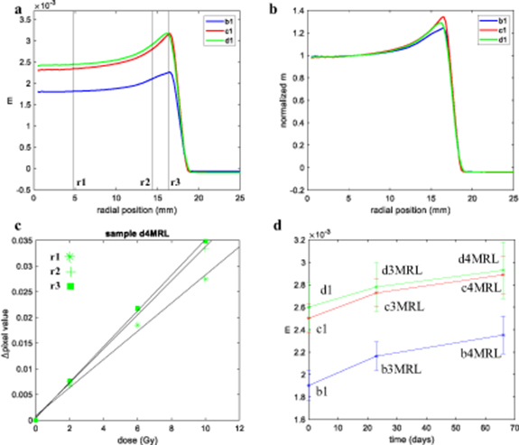
Figure A1. (a) Absolute values and (b) normalized relationship between gradient and radial position obtained with samples from Formulation b, c and d in a conventional linac (samples b1, c1 and d1). Over-responses at the edge are 34%, 29% and 23% respectively. (c) Dose-response relations show reduced linearity. (d) Relationship between averaged absolute gradient and time of irradiation post-manufacture for all the uniformly irradiated calibration samples. Time represents the number of days between the sample manufacture and their irradiation. All samples shown here were manufactured at the same time. Error bars represent one standard deviation of the gradient values found in a cylindrical subvolume of radius ∼1.75 cm of each sample.
Download figure:
Standard image High-resolution image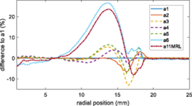
Figure B1. Difference between sample a1 normalized m values and samples a2 (irradiated at the same time), a3–a5 (irradiated 2.6 months after), a6 (irradiated 7.1 months after) and a11MRL (irradiated 7.9 months after).
Download figure:
Standard image High-resolution image
Figure B2. Transverse and longitudinal profiles averaged over the middle of sample a1, after being reduced in diameter (+ cut) and then irradiated with additional 6 Gy (+ cut+ 6 Gy), and scanned again after a month (cut + 6 Gy+ 1 month), are shown after normalization to the flat region of each reconstructed image. Changes in the extension of the axial edge effect (+ 1.4 mm) are visible a month after the second irradiation. During this time the sample was in the fridge and in the dark.
Download figure:
Standard image High-resolution image
Appendix B.: Edge-effect over time
It was not the aim of this manuscript to study dose sensitivity changes systematically over time for all samples, but our preliminary anecdotal result is that the extent of the edge effect increases as samples age. The difference in the normalized gradient between samples a22–a6 and a11MRL when compared to sample a1, showing the magnitude and extent of the edge effect at different time points is shown in figure B1. As noted in the main body of the text, samples a2 to a5 differ from a1 for inter-batch and other reasons. However the changes seen in samples a6 and a11MRL are larger and it is clear that the effect has extended further into the sample. Changes in the edge effect magnitude for sample a1 after being reduced in diameter and irradiated uniformly after with 6 Gy are shown in figure B2.