
Abstract
In-room imaging is a prerequisite for adaptive proton therapy. The use of onboard cone-beam computed tomography (CBCT) imaging, which is routinely acquired for patient position verification, can enable daily dose reconstructions and plan adaptation decisions. Image quality deficiencies though, hamper dose calculation accuracy and make corrections of CBCTs a necessity. This study compared three methods to correct CBCTs and create synthetic CTs that are suitable for proton dose calculations. CBCTs, planning CTs and repeated CTs (rCT) from 33 H&N cancer patients were used to compare a deep convolutional neural network (DCNN), deformable image registration (DIR) and an analytical image-based correction method (AIC) for synthetic CT (sCT) generation. Image quality of sCTs was evaluated by comparison with a same-day rCT, using mean absolute error (MAE), mean error (ME), Dice similarity coefficient (DSC), structural non-uniformity (SNU) and signal/contrast-to-noise ratios (SNR/CNR) as metrics. Dosimetric accuracy was investigated in an intracranial setting by performing gamma analysis and calculating range shifts. Neural network-based sCTs resulted in the lowest MAE and ME (37/2 HU) and the highest DSC (0.96). While DIR and AIC generated images with a MAE of 44/77 HU, a ME of −8/1 HU and a DSC of 0.94/0.90. Gamma and range shift analysis showed almost no dosimetric difference between DCNN and DIR based sCTs. The lower image quality of AIC based sCTs affected dosimetric accuracy and resulted in lower pass ratios and higher range shifts. Patient-specific differences highlighted the advantages and disadvantages of each method. For the set of patients, the DCNN created synthetic CTs with the highest image quality. Accurate proton dose calculations were achieved by both DCNN and DIR based sCTs. The AIC method resulted in lower image quality and dose calculation accuracy was reduced compared to the other methods.
Export citation and abstract BibTeX RIS

Original content from this work may be used under the terms of the Creative Commons Attribution 3.0 license. Any further distribution of this work must maintain attribution to the author(s) and the title of the work, journal citation and DOI.
1. Introduction
Adaptive radiotherapy (ART) intends to improve radiation treatments by monitoring changes in patient anatomy, assessing the actual delivered dose and subsequently modifying treatment plans to achieve the best possible target coverage and organs at risk sparing (Yan et al 1997, Lim-Reinders et al 2017, Sonke et al 2019). Repeated imaging throughout the treatment course plays an essential role in adaptive treatment strategies, since dose recalculations, based on these images, indicate the necessity for treatment plan modifications (Hvid et al 2018, Posiewnik and Piotrowski 2019).
In photon therapy centers, and in recent years also in proton therapy centers, on-board cone-beam computed tomography (CBCT) systems are available for accurate pre-treatment patient alignment (Hua et al 2017, Stock et al 2018). Beside patient position, CBCT images can also provide information about interfractional changes of the patient anatomy.
Accurate stopping power ratios (SPR), which are typically derived from CT numbers, are a prerequisite for precise proton dose calculations. The relationship between CT-number and SPR is ambiguous and not unique since tissues with similar CT-numbers can have different SPRs and vice versa (Yang et al 2012). Any underlying CT-number error will enlarge the uncertainty of the SPR conversion and eventually affect dosimetric accuracy. This makes proton dose calculations in particular sensitive to CT-number uncertainties. In contrast to conventional fan-beam CT, cone-beam CT images suffer from various imaging artifacts that impair the image quality and lead to such CT-number uncertainties (Schulze et al 2011, Nagarajappa et al 2015). Due to the high requirements on the accuracy of CT-numbers, clinical proton dose calculations cannot be performed directly on CBCT images and corrections have to be applied to the CBCTs first.
With a rise in CBCT equipped proton therapy centers and the increased interest in adaptive proton therapy in recent years, different correction approaches and their suitability for proton dose calculations have been reported in literature. This includes, among others, look-up table (LUT) based approaches (Kurz et al 2015), histogram matching (Arai et al 2017), deformation of planning CTs (Peroni et al 2012, Veiga et al 2015, 2017, Landry et al 2015b, Veiga et al 2016), projection-based correction methods (Niu et al 2010, Park et al 2015, Kurz et al 2016a) and deep learning techniques (Kida et al 2018, Hansen et al 2018).
Kurz et al investigated a LUT based CBCT correction method (2015). This relatively simple technique was found not sufficiently accurate for proton dose calculations and was outperformed by a deformable image registration method. Results from a histogram matching algorithm were reported by Arai et al (2017). In this study, dose calculation accuracy in phantoms and head and neck cancer patients was improved compared to dose calculation on raw CBCTs. Another approach, that was comprehensively investigated in the context of adaptive photon radiotherapy, is the deformation of planning CTs onto the geometry of daily CBCTs which results in a synthetic CT (often also referred to as virtual CT or pseudo CT). In the scope of proton therapy of lung malignancies, Veiga et al reported findings from such a deformable image registration method (2015, 2016, 2017). They concluded that for lung cancer similar conclusions for plan adaptations can be drawn on a synthetic CT as on a repeat (fan-beam) CT scan. Their method also incorporated additional correction steps for areas in which the deformable image registration was not able to reconstruct correctly. For head and neck cancer patients Landry et al reported good agreement between dose calculated based on a synthetic CT resulting from deformed planning CT and on a repeat CT (2015b). Kurz et al compared the deformable image registration method to a projection based correction method in terms of its suitability for proton dose calculations (2016a). The projection-based method was initially described by Niu et al (2010) and Park et al (2015). It uses the synthetic CT, created by deformable image registration, as prior for scatter correction and was found highly accurate in terms of proton dose calculations. Kurz et al concluded that for head and neck patients, the synthetic CTs from the deformable image registration method were equally suitable for proton dose calculations than those from the projection-based correction method. For prostate cancer patients, the projection-based method performed better.
With the recent progress in the field of artificial intelligence (AI), such techniques are increasingly applied to problems in radiology and radiotherapy. In the subfield of medical image synthesis a lot of progress has been recently made using AI to convert magnetic resonance (MR) images into synthetic CT images (Han 2017, Chen et al 2018). These techniques have also been translated to CBCT scatter correction. AI-based CBCT correction methods include conventional machine learning techniques such as random forest based methods (Li et al 2019) but also deep learning based methods like deep convolutional neural networks (Kida et al 2018) and generative adversarial networks (Liang et al 2019, Harms et al 2019). In random forest-based methods decision trees are trained to predict CT intensities based on aligned CT and CBCT or MRI patches. Deep convolutional neural networks, on the other hand, learn a direct non-linear mapping of image intensities from one imaging modality to another using paired CBCT and CT images. Generative adversarial networks have the ability to learn from unpaired CBCT and CT datasets. A common advantage of all these AI-based techniques is that they do not require a planning CT for sCT generation once the model is trained.
Kida et al showed one of the first applications of deep learning approaches to convert CBCT images into synthetic CTs (2018), but did not include a dosimetric evaluation. Li et al reported high image quality and potential for accurate dose calculations of DCNN based synthetic CTs for photon radiotherapy (2019). Hansen et al evaluated the accuracy of proton dose calculations on CBCTs corrected with a U-net deep convolutional neural network which was trained on raw and scatter-free CBCT projections (2018). For patients with pelvic tumors, their results showed insufficient proton dose calculation accuracy. Landry et al used a similar convolutional neural network and compared different training data types (2019). This included raw and scatter-free projections, reconstructed CBCTs, DIR-synthetic CTs and reconstructed CBCTs, based on raw and corrected projections. For proton dose calculations in prostate cancer patients the method using CBCTs, from raw and corrected projections, performed best. Table 1 summarizes the methods for synthetic CT creation, the anatomical site for which they were evaluated and their suitability for proton dose calculations.
Table 1. Overview of previously investigated CBCT correction/conversion methods in the context of proton dose calculations.
| Method | Literature | Anatomical site | Suitability for proton dose calculation |
|---|---|---|---|
| LUT based correction | Kurz et al 2015 | Head and neck | — |
| Histogram matching | Arai et al 2017 | Phantoms, head and neck | — |
| DIR | Veiga et al 2015, 2016, 2017, Kurz et al 2015, 2016a, Landry et al 2015b | Lung, head and neck, pelvis | ++ (H&N), + (pelvis), + (lung) |
| Projection-based correction | Park et al 2015, Kurz et al 2016a | Head and neck, pelvis | ++ |
| Deep convolutional neural network | Hansen et al 2018, Landry et al 2019 | Pelvis | + |
— stands for insufficient, + for acceptable, and ++ for high proton dose calculation accuracy.
A comparison of the above-mentioned methods is challenging since many investigations were carried out for different anatomical regions, were based on different input data and used different metrics for the dosimetric evaluation. In this work, we compare three methods to correct CBCTs (acquired in a proton treatment room) and create synthetic CTs using a large head and neck data set. Method 1 uses a deep convolutional neural network derived by the work of Spadea et al (2019). Method 2 is based on deformable image registration and uses a similar DIR-algorithm as Veiga et al, Kurz et al and Landry et al (Landry et al 2015b, Veiga et al 2016, Kurz et al 2016a). Method 3 uses an iterative approach where the joint histogram between the pCT and the CBCT is used to create an intensity conversion function. Shading artifacts are also corrected by using a correction map constructed utilizing the planning CT. Results from the various methods are compared in terms of image quality and proton dose calculation accuracy.
In a clinical context, not only raw performance and accuracy are predominant factors to determine if a method is suitable for clinical implementation. Stability, time consumption, and labor efficiency should also be considered. Our work aims at identifying a clinically optimal method to create synthetic CTs suitable for an automated adaptive proton therapy workflow. Compared to previous works, multiple sCT methods are tested on exactly the same extensive dataset. This facilitates an in-depth comparison of these methods for application in adaptive proton therapy.
2. Material and methods
2.1. Patient data
CT and CBCT imaging data from 33 head and neck cancer patients, treated with PBS proton therapy at the University Medical Center Groningen (UMCG, Netherlands), were used to create synthetic CTs (sCT). Images were acquired between January 2018 and February 2019 and patients were aged between 27 and 80 years (mean: 62 years). Out of the 33 patients, 23 were of male gender. A planning CT (pCT), acquired approximately three weeks before treatment, weekly repeated CTs (rCT) and daily CBCTs (used for patient position verification), were available for each patient. For synthetic CT generation and validation, CBCT-CT imaging pairs from the day of the first rCT acquisition were chosen. A Siemens SOMATOM Definition AS Open scanner (Siemens Healthineers, Germany) with a resolution of 0.98 mm × 0.98 mm, a slice thickness of 2 mm and a FOV of 500 mm was used for the acquisition of the pCTs. For rCTs, a Siemens SOMATOM Confidence scanner with similar settings (resolution: 0.98 mm × 0.98 mm, slice thickness: 2 mm, FOV: 500 mm) was utilized. CBCT images were acquired using the onboard imaging device of an IBA Proteus®PLUS gantry (IBA, Belgium). CBCTs were reconstructed on a 0.50 × 0.50 mm × 2.50 mm grid with a FOV of 260 mm. Generally, CBCTs consisted of 140 and CTs of 226 axial slices. Both with an axial resolution of 512 × 512 pixels. A facial mask was used during CBCT and CT acquisition to fix the patient's head in a reproducible position.
CT and CBCT images were not covering the same field-of-view (FOV) and were therefore cropped to an equal FOV during data preparation. Furthermore, the low dose imaging protocol for CBCT acquisition lead to artifacts and heavily impaired image quality below the shoulders. To avoid any influence on the image and dose comparison, we cropped this region on all images. Examples for the extent of image cropping can be found in section S4 of the supplementary materials (stacks.iop.org/PMB/65/095002/mmedia).
2.2. sCT methods
2.2.1. Neural network method (NN)
Paired CBCT and rCT images, acquired on the same day with the same immobilization, were used to train a deep convolutional neural network (DCNN) to convert CBCT image intensities into CT intensities, generating sCTs. The employed network was originally designed for MRI to sCT conversion but was left unchanged for our purpose (Spadea et al 2019). It is based on a U-net proposed by Han (2017). This U-net consists of an encoding path to extract representative features from the CBCT using convolutional layers. This encoding path is followed by a decoding path, also based on convolutional layers, to reconstruct these features with the corrected HUs. Based on this architecture, Spadea et al further introduced a multi-planar approach to train an individual network for axial, sagittal and coronal images which are afterwards combined into a final sCT image. A detailed description of the applied neural network in the context of MRI based sCT synthesis was reported by Spadea et al (2019).
Before training the neural network various data preparation steps were necessary. On the CBCT and rCT the treatment couch, facial mask, and background were removed by segmenting the patient outline using an automatic segmentation algorithm included in the image processing software Plastimatch www.plastimatch.org; Zaffino et al 2016. The resulting masks were manually corrected to assure complete coverage of ears, nose and lungs. All voxels outside these masks were set to −1000 HU. As a next step a rigid registration of the CBCT to the rCT was performed using the registration algorithm included in Plastimatch. In the last step, the CBCT was deformably registered to match the rCT using a diffeomorphic morphons DIR algorithm (Janssens et al 2011) included in the openREGGUI MATLAB package www.openreggui.org. This resulted in aligned images to train the neural network. To allow a meaningful comparison, the resulting pre-processed CBCT was also used as starting points for the other two methods. For simplification, we will still refer to it as CBCT, although it is not the original CBCT anymore. Synthetic CTs resulting from the DCNN training will be referred to as sCTNN in the following sections.
As described by Spadea et al (2019), three individual sets of weights were trained using slices from axial, sagittal or coronal views, respectively. The resulting images from each trained network were combined afterwards. The training was performed on a NVIDIA 1080 Ti Graphical Processing Unit (GPU). In total, including slices from all views and data augmentation, 240 thousand slices were used to optimize 32 million learnable parameters of the DCNN. The data augmentation included small translations and mirroring of entire slices. The training was stopped when five consecutive epochs did not improve the validation loss.
A 3-fold cross-validation approach was followed by randomly splitting our dataset into three subsets of 11 patients each. Two subsets were used for training/validation, while the third was used for testing of the trained network. This was repeated two times, so every subset was used for testing once. This procedure allowed the utilization of all 33 patients as testing cases and increased the number of available patients for image comparison and dosimetric evaluations.
2.2.2. Deformable image registration method (DIR)
As a second method to generate synthetic CTs, a diffeomorphic morphons DIR algorithm, implemented in the MATLAB package openREGGUI, was used to deform the pCT onto the geometry of the CBCT. This algorithm is particularly suited for CBCT-CT image registration since it is using a local phase metric instead of solely focusing on image intensities (Kurz et al 2016a). The algorithm was previously applied for CBCT-CT image registration and showed suitability for H&N applications (Landry et al 2015a, Kurz et al 2016b). Before DIR the patient outline was automatically segmented on CBCT and pCT using Plastimatch. Similar to the neural network data preparation, masks were checked manually to assure full coverage and values outside the patient outline were set to −1000 HU. Afterwards, the pCT was rigidly registered to the CBCT and the FOV was cropped to be equal to the FOV of the CBCT. Then the actual CBCT conversion was performed by deforming the pCT to match the CBCT. We refer to the resulting image as sCTDIR.
2.2.3. Analytical image-based correction method (AIC)
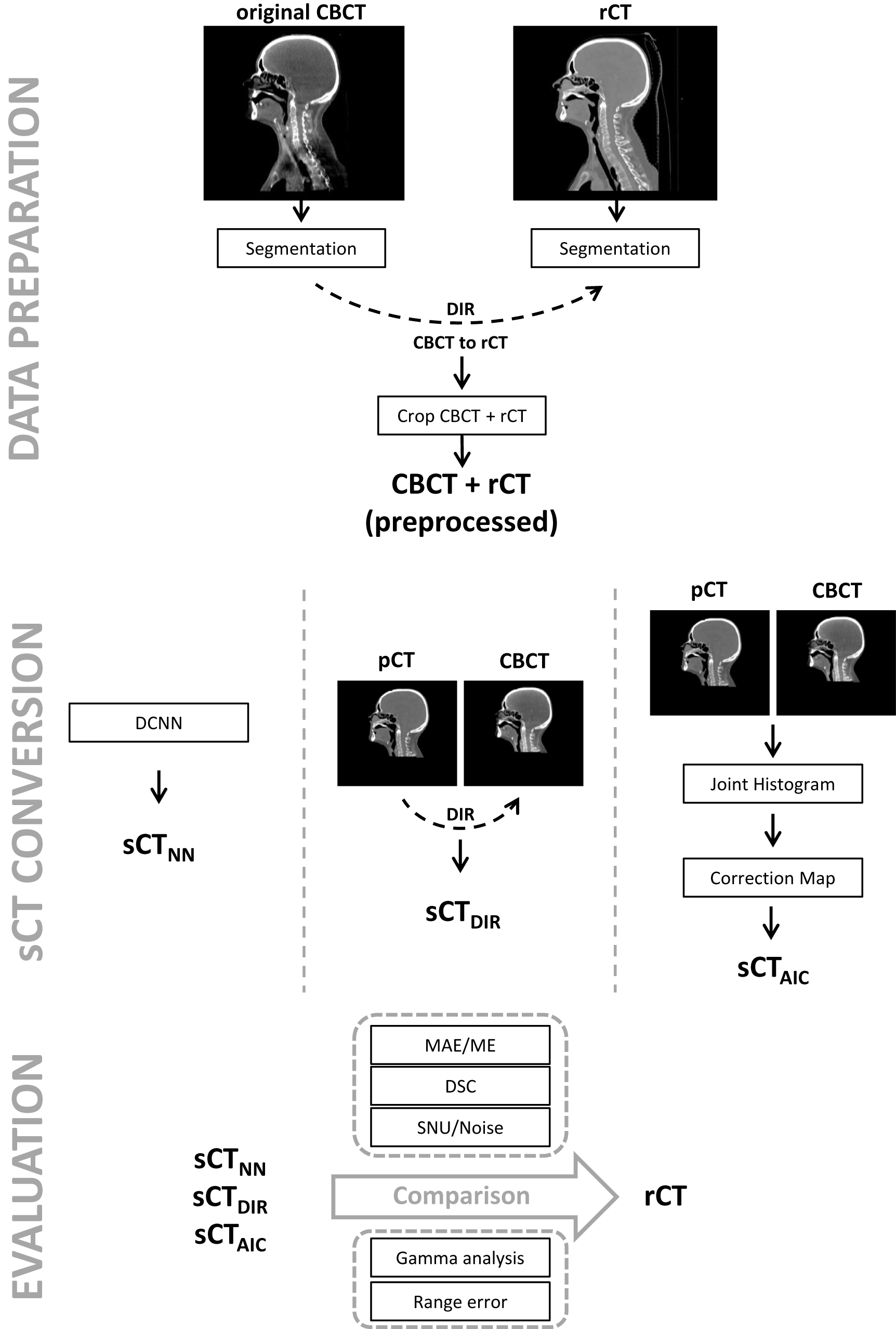
A first version of an analytical correction and conversion method was available in a research version of the clinical treatment planning system (TPS) Raystation (Version 7.99; RaySearch, Sweden). This third investigated method uses an iterative approach to convert and correct CBCTs. First, the pCT is utilized to find a conversion from CBCT to CT intensity scale by creating a joint histogram in which points corresponding to different tissues are found and a piecewise linear conversion function is created. Then, image artifacts are reduced by creating a correction map, not influenced by anatomical differences, that tries to eliminate low-frequency variations that are present on the CBCT but not on the pCT. As data preparation, the pCT was rigidly registered to the CBCT and masked to cover the same FOV as the CBCT. For optimal results, the recommendation to perform a DIR within the TPS was followed. After that, the script was executed and resulted in sCTAIC. An overview of the data preparation steps for all methods is provided in figure 1.

Figure 1. Overview of data preprocessing, sCT conversion and data evaluation. sCT = synthetic CT, rCT = repeated CT, DIR = deformable image registration, DCNN = deep convolutional neural network, AIC = analytical image-based correction, MAE = mean absolute error, ME = mean error, DSC = dice similarity coefficient, SNU = spatial non-uniformity index.
Download figure:
Standard image High-resolution image2.3. Image evaluation
The rCT was used as 'ground truth' image to evaluate the performance of the various sCT conversion methods. The image quality and accuracy of the CBCT-conversion methods were quantified by mean absolute error (MAE) and mean error (ME), defined in equations (1) and (2).


Only voxels that lay within the automatically created patient skin contour were considered for MAE and ME calculations. A distribution of the MAE in varying HU regions was investigated by calculating a MAE-spectrum for bins of 20 HU from −1000 to 1500 HU. To assess the geometric accuracy of each conversion method, the Dice similarity coefficient (DSC) was calculated for bone according to equation (3). For this purpose, a segmentation of bone tissue was performed by thresholding the images to only include voxels with HU-values above a certain limit. Threshold values from 100 to 1000 HU (in steps of 100 HU) were used to calculate a DSC spectrum. This allowed an investigation of the similarity of bone tissues with increasing density.

Furthermore we investigated the DSC of air cavities within the patient outline. To segment the air cavities on the rCT and sCTs we used a threshold of −465 HU (Nakano et al 2013) and calculated the DSC according to equation (3).
The spatial uniformity of CBCT images is impaired by scatter artifacts. We therefore calculated the spatial non-uniformity index (Shi et al 2017, Kida et al 2018) for the original CBCT, the reference rCT and the various sCTs. The spatial non-uniformity (SNU) is defined as

where  is the maximum/minimum of the mean pixel value out of multiple ROIs located in regions with similar density. In this work, six ROIs were equally distributed across the soft tissue in the brain. An example for the ROI-positioning can be found in the supplementary materials subsection S2. A low SNU index indicates high uniformity across the image.
2.4. Dosimetric evaluation
To evaluate the suitability of the sCTs for proton dose calculations, two pencil beam scanning (PBS) proton plans with artificial target volumes were created in the research version of RayStation TPS (version 7.99). For plan 1, a cylindrical target was positioned in the region of the brainstem and was treated with a beam incoming from a 45° gantry angle (see figure 2(b)). This direction was chosen to avoid airways and oral cavity, where movements and anatomical variations occur frequently and on short timescales. Nonetheless, the beam still traverses a challenging path with small bone structures and multiple bone-soft tissue interfaces. For plan 2, a target with a larger volume was positioned above the first one in a central location in the brain. It was irradiated from a 180° gantry angle and only traverses the skull and brain (see figure 2(c)). In plan 2, the beam passes through the skull and then stops in brain tissue. Four patients had to be excluded from the dosimetric evaluation using plan 2. This was caused by the limited FOV of the CBCTs at the posterior part of the skull.

Figure 2. (a) Exemplary targets used in plan 1 (blue, inferior) and plan 2 (yellow, superior), (b) beam direction for plan 1, (c) beam direction for plan 2.
Download figure:
Standard image High-resolution imageFor both targets, a uniform dose of 10 GyRBE in five fractions (5 × 2 GyRBE) was planned on a 1 mm × 1 mm × 1 mm dose grid. A constant RBE value of 1.1 was used for all dose calculations. Figure 2 depicts the target positions and beam directions. The average target volumes for plans 1 and 2 were 20 and 50 cm3, respectively.
Initially, the dose was calculated on the rCT using the RayStation Monte Carlo dose engine with an uncertainty of 1.0%. For the dosimetric evaluation, the dose was then recalculated on sCTNN, sCTDIR and sCTAIC. Gamma pass ratios, including only voxels above 10% of the prescribed dose, were computed for 2%/2 mm and 3%/3 mm criteria. Furthermore, a comparison of HU-profiles of rCT, sCTNN, sCTDIR and sCTAIC and the resulting dose profiles were plotted along the beam direction at a central line of plan 1 and 2.
To further investigate the proton dose calculation accuracy of the synthetic CTs, range shifts were computed by comparing depth-dose profiles from dose calculations based on the rCTs and the synthetic CTs as in Pileggi et al (2018). Range shifts were determined by shifting the depth-dose profile until the sum of differences between the two curves was minimal. This was performed for all dose profiles that were exposed to at least 80% of the planned dose. Based on these results, the mean and standard deviation of the relative range shift for each patient and the entire patient population were calculated.
3. Results
3.1. Image quality and time efficiency
3.1.1. Neural network (NN)
On average, the training of the DCNN was stopped after 29 epochs. Table 2 shows the number of epochs that each network was trained for and the resulting MAE and ME for the individual subsets of the 3-fold cross-validation. Training of one epoch took up to 4 h. With the hardware used during this study, converting a CBCT into a sCT took about 3 min (1 min per view). Time for combining the views was negligible. sCTNN resulted in an average MAE and an average ME of 36.3 ± 6.2 HU and 1.5 ± 7.0 HU, respectively.
Table 2. Overview of training epochs for subset 1–3 in axial, sagittal and coronal views. Additionally, also the MAE and ME for the individual subsets are listed.
| Nr. of epochs | MAE [HU] | ME [HU] | |||
|---|---|---|---|---|---|
| Axial | Coronal | Sagittal | |||
| Subset 1 | 35 | 32 | 31 | 36.4 ± 5.6 | 0.9 ± 5.1 |
| Subset 2 | 29 | 25 | 23 | 34.9 ± 3.7 | 2.0 ± 7.1 |
| Subset 3 | 31 | 27 | 26 | 37.8 ± 8.4 | 1.4 ± 8.2 |
3.1.2. Deformable image registration (DIR)
Generating synthetic CTs by deforming the pCT onto the CBCT took about 20 min per patient and resulted in an average MAE of 44.3 ± 6.1 HU and an average ME of −7.6 ± 4.9 HU.
3.1.3. Analytical image-based correction (AIC)
For synthetic CTs created with the AIC method, MAE and ME averages of 76.2 ± 13.3 HU and 1.4 ± 11.5 HU were observed. Conversion times, including the deformable registration in the TPS, lay between 1 and 2 min. After registration, the actual conversion from CBCT to sCTAIC was very fast and only required 5–10 s of computational time.
3.2. Image comparison
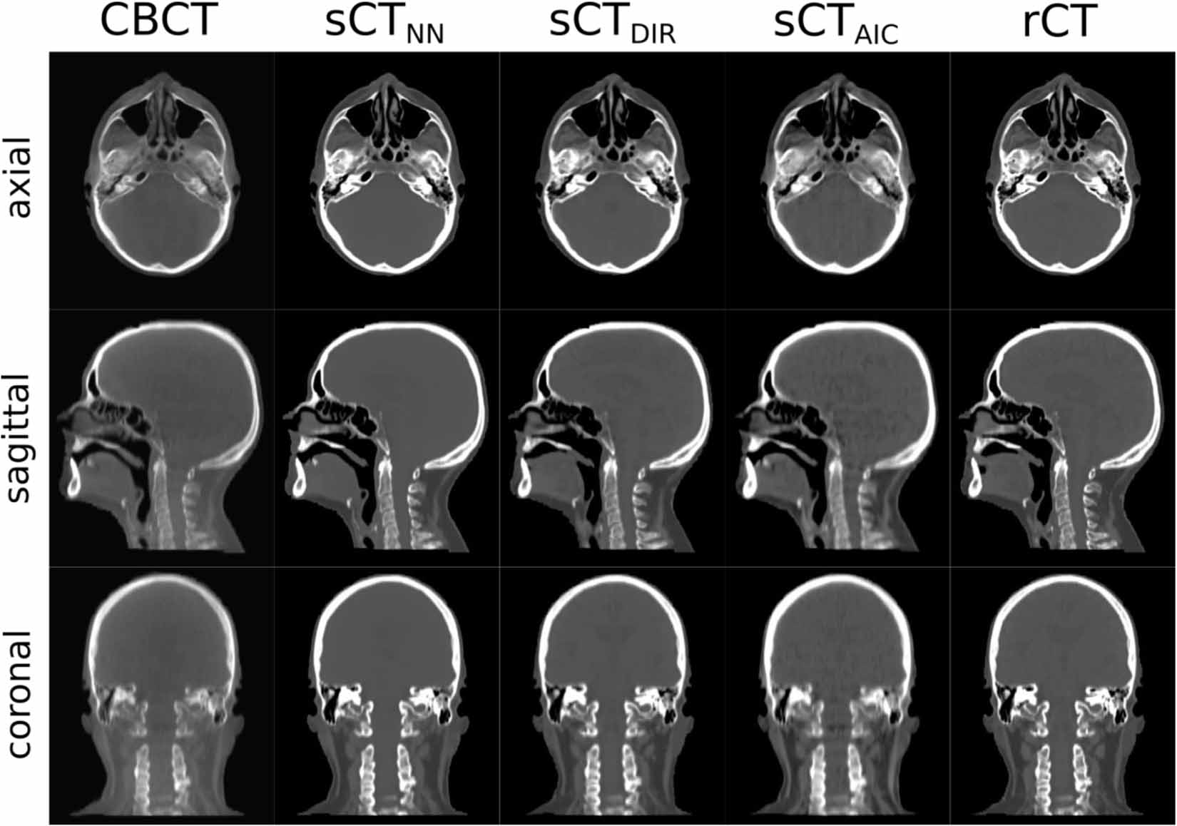
Figure 3 provides an overview of the CBCT, the created synthetic CTs and the reference rCT for patient 15 in axial, sagittal and coronal views. A Hounsfield-unit window of 2000/0 was applied to all images. sCTAIC images were noticeably blurrier than sCTNN and sCTDIR images. This was partially caused by resampling and image registration of the CBCT during preprocessing. Image noise was comparable to the rCT in sCTDIR, lower in sCTNN and higher in sCTAIC. A quantitative analysis of imaging noise in different tissues and animated figures showing the entire imaging volumes can be found in subsections S2 and S3 of the supplementary materials.

Figure 3. Comparison of CBCT, the various sCTs (sCTNN, sCTDIR and sCTAIC) and the reference rCT images in axial, sagittal and coronal views for patient 15. The same HU-windowing settings [WL = 250,WW = 1250] were applied to all images except for the CBCT, where a window of [1900,−100] was used. The MAE values for this patient are: sCTNN = 35.8 HU, sCTDIR = 43.4 HU and sCTAIC = 78.2 HU. Gamma pass ratios(2%/2 mm) are: sCTNN = 99.2%, sCTDIR = 99.5% and sCTAIC = 98.4%.
Download figure:
Standard image High-resolution imageFigure 4 presents the difference between rCT and the various synthetic CTs for patient 15. The higher average MAE of sCTAIC is clearly visible in all views. Especially in bone, the error is larger than for the other two methods. In sCTNN the error is more randomly distributed than in sCTDIR and sCTAIC, where the error is mostly distributed around bone/soft-tissue interfaces. This is partially caused by the use of deformable image registration to create synthetic CTs. High error areas can also be seen in the oral and nasal cavity. However, these errors are caused by actual anatomical differences between the CBCT and the ground truth rCT and not by the synthetic CT conversion itself.

Figure 4. Difference images between rCT and the various sCT methods in coronal, sagittal and axial view of patient 15. The color bar indicates the difference in HU.
Download figure:
Standard image High-resolution imageFigures 5(a) and (b) present the MAE and ME of the three conversion methods for the entire dataset. All datasets were visually checked for any impeding factors. Due to major imaging artifacts, the CBCT of patient 4 was found not suitable for further investigation and was therefore excluded from all further analysis. sCTNN produced images with the lowest MAE for all cases. On average, the MAE was 8 HU higher for sCTDIR and 40 HU higher for sCTTPS. For sCTNN (1.5 HU) and sCTAIC (1.4 HU), the ME was evenly distributed around zero, while for sCTDIR (−7.6 HU) the ME was noticeably shifted towards lower HU values. Due to a specific neck position of patient 18, the conversion using the AIC method partially failed and increased MAE and ME values were observed.

Figure 5. (a) Mean absolute error (MAE) and (b) mean error (ME) in HU of sCTNN, sCTDIR and sCTAIC for all 33 patients. Only voxels within the patient outline were considered for calculation of MAE and ME.
Download figure:
Standard image High-resolution imageFigure 6 reports the average MAE spectrum for sCTNN, sCTDIR and sCTAIC. The shaded areas indicate the standard deviation within the entire patient dataset. For voxels with HUs in the interval from −1000 to 0, sCTNN resulted in the lowest average MAE, though the standard deviation overlaps with sCTDIR and sCTAIC. For HUs above 0, sCTAIC shows double the error than sCTNN and sCTDIR. The trend of sCTDIR and sCTTPS with increasing HU is similar while sCTNN exhibits a different behavior with a decreasing MAE above 1000 HU. Overlapping with the MAE-spectrum, also an average image histogram is presented in figure 6. It shows that most of the voxels have CT-numbers around 0 HU and hence the global MAE is also mainly determined by these voxels.

Figure 6. Mean absolute error spectrum for sCTNN, sCTDIR and sCTTPS. The continuous lines were created by binning the MAE (bin-size 20 HU), calculating MAE for every bin and averaging over all patients (excluding patient 4). Shaded areas indicate one standard deviation. The dashed black line shows an average image histogram.
Download figure:
Standard image High-resolution imageFigure 7 shows the DSC of bone tissue for a range of threshold values. At a threshold of 200 HU, sCTNN results in a DSC of 0.96, sCTDIR in 0.95 and sCTAIC in 0.90. With increasing threshold values, representing more dense bone tissue, the DSC decreases.

Figure 7. DSC for threshold values between 100 and 1000 HU. Averaged over all patients (excluding patient 4). Error bars indicate 1 SD.
Download figure:
Standard image High-resolution imageFor air cavities an average DSC of 0.90, 0.81 and 0.80 was observed for sCTNN, sCTDIR and sCTAIC, respectively. These values are significantly lower than the once observed for bone. This is caused by variations in the oral cavity that occur between scans even if acquired on the same day.
For rCT, CBCT, sCTNN, sCTDIR and sCTAIC we observed an average SNU of 14.0 ± 7.0 HU, 118.0 ± 45.0 HU, 8.5 ± 4.2 HU, 12.4 ± 6.1 HU and 21.6 ± 16.3 HU, respectively. These results show that all three sCT methods significantly reduce the non-uniformity caused by scatter on the CBCT. As expected, the lowest difference to the ground truth rCT was observed for sCTDIR since it deforms a planning CT scan with similar uniformity as the rCT. sCTAIC resulted in images with lower uniformity than the rCT scan, while the smoothing and the loss of detail in the soft tissue of the brain leads to a higher uniformity for sCTNN when compared to the rCT and all other sCT methods.
3.3. Dosimetric evaluation
Figure 8(a) shows HU profiles and corresponding line doses of dose distributions based on the rCT, sCTNN, sCTDIR and sCTAIC along the beam direction of plan 1. sCTNN and sCTDIR profiles closely follow the HU profile of the rCT, but show some locally confined differences. Larger deviations could be observed for the HU-profile of sCTAIC which resulted in higher range shifts for dose distributions based on the sCTAIC. Although, it has to be noted that in the selected profile the range shift of sCTAIC is larger than the overall average range shift of sCTAIC. Hence, it is not representative for the entire dataset.

Figure 8. Comparison of Hounsfield unit (HU) profiles of rCT, sCTNN, sCTDIR and sCTAIC along a) beam direction 1 and b) beam direction 2 for patient 15. Dashed lines represent dose profiles of the according sCTs. The presented profiles are exemplary and are not representative of the entire dataset.
Download figure:
Standard image High-resolution imageFigure 8(b) presents a similar plot for profiles in the beam direction of plan 2. In this case, all three methods can reproduce HU-values of the rCT in the homogeneous soft tissue areas. Higher noise was observed for sCTAIC. sCTNN achieves the highest agreement with the rCT. sCTDIR is not able to reconstruct the first peak accordingly. This is partially connected to the deformation of the pCT that also causes a deformation of the patient outline. sCTAIC underestimates the HU of the first peak but also overestimates the HU of the second peak. Overall, this results in no range shift for the dose recalculated on sCTAIC.
Table 3 presents the gamma analysis results using 2%/2 mm and 3%/3 mm acceptance criteria for both plans. Boxplots in figure 9 indicate the distribution of the pass ratios for the entire dataset. While sCTNN showed a similar distribution of pass ratios for plan 1 and 2, sCTDIR and sCTAIC have a noticeably wider distribution in plan 2.
Table 3. Overview of average gamma pass ratios for 1%/1 mm, 2%/2 mm and 3%/3 mm criteria. In brackets minimum and maximum values of each method/criteria are listed.
| Plan 1 | Plan 2 | |||
|---|---|---|---|---|
| 2%/2 mm [min, max] | 3%/3 mm | 2%/2 mm | 3%/3 mm | |
| sCTNN | 99.43 [98.08, 99.75] | 99.98 [99.75, 100] | 99.18 [93.75, 99.57] | 99.91 [99.70, 100] |
| sCTDIR | 99.58 [97.59, 99.84] | 99.96 [99.10, 100] | 98.35 [87.52, 99.62] | 99.84 [93.60, 99.99] |
| sCTAIC | 98.05 [95.39, 99.62] | 99.66 [98.48, 100] | 96.64 [84.87, 99.44] | 99.23 [93.48, 99.98] |

Figure 9. Boxplots of gamma pass ratios (2%/2 mm) of sCTNN, sCTDIR and sCTAIC for (a) plan 1 and (b) plan 2.
Download figure:
Standard image High-resolution imageThe range shift analysis for plan 1 resulted in a mean relative range shift of 0.0 ± 0.7%, 0.1 ± 0.4% and −0.8 ± 1% for sCTNN, sCTDIR and sCTAIC, respectively. For plan 2, a mean relative range shift of −0.1 ± 0.3%, −0.6 ± 0.7% and −0.3 ± 1.6% was observed for sCTNN, sCTDIR and sCTAIC. In both plans, sCTNN resulted in the lowest mean range error. The lowest standard deviation in plan 1 was observed for sCTDIR, in plan 2 for sCTNN. Figure 10 presents boxplots of range errors for individual patients. It visualizes the higher standard deviations of sCTNN and sCTAIC when compared to sCTDIR in plan 1. Contrary to sCTDIR and sCTAIC, plan 2 resulted in lower range shifts for sCTNN. sCTDIR and sCTAIC showed increased inter-patient variability in plan 2.

Figure 10. Boxplots of relative range errors for plan 1 (a) and plan 2 (b) for every patient individually. In figure 10(b) whiskers are out of the image frame for patients 3 (value of −6.5%), 17 (−6.9%), 19 (−5.5%) and 32 (−8.2%).
Download figure:
Standard image High-resolution image3.4. Patient-specific differences
Besides global differences between the various synthetic CT methods, also patient-specific variations were observed. Figure 11 presents a selection of these variations to further highlight differences between the synthetic CT methods. Figure 11(a) shows minor dental artifacts of patient 19. On the ground-truth rCT (and also the pCT) these artifacts are not visible because built-in iterative metal artifact correction was used. This technique was not available on the used CBCT scanner. sCTNN and sCTDIR were able to completely compensate for the dental artifacts, while sCTAIC still suffered from these artifacts in a similar magnitude as the CBCT. Figure 11(b) depicts more pronounced dental artifacts on the CBCT of patient 26. These artifacts are in a reduced intensity also visible on the rCT. On sCTNN the artifact was almost reduced to rCT level. Similar to patient 19, sCTAIC shows artifacts in the same magnitude as on the CBCT. In total 42% of the patients used in our work showed some kind of dental artifact.

Figure 11. Patient-specific differences of the various sCT methods. (a), (b) Dental artifacts, (c) artifact from nasogastric tube, (d) filling of sphenoid sinus on sCTDIR.
Download figure:
Standard image High-resolution image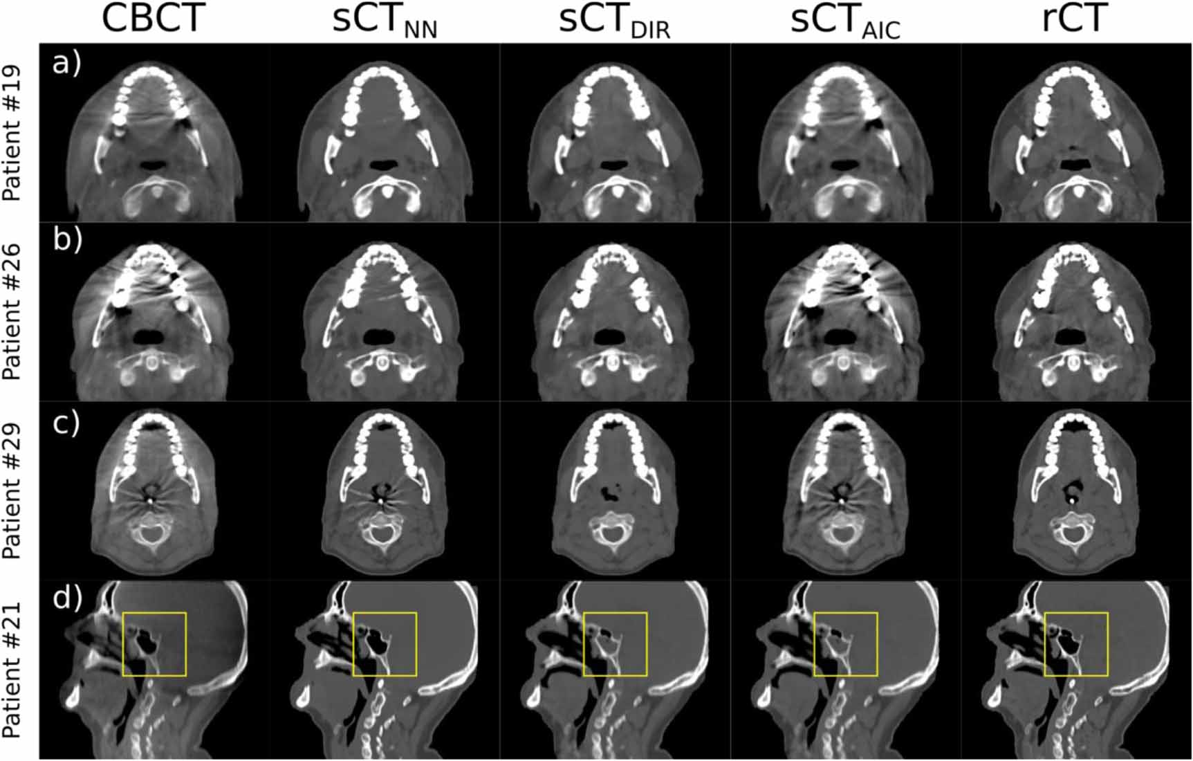
In figure 11(c), a nasogastric tube is visible on the CBCT and the rCT of patient 29. This tube lead to an artifact that is present on the CBCT but not on the rCT. On sCTDIR no artifact but also no nasogastrical tube is visible. This was caused by not using such a tube during pCT acquisition, which was then deformed to create sCTDIR. On sCTNN and sCTAIC these artifacts are still visible and uncorrected. Contrary to the dental artifact, which was present in multiple patient cases, the artifact emerging from the nasogastric tube was only seen in a single patient case.
Patient 21, shown in figure 11(d), has a filled sphenoid sinus (indicated by yellow box) on sCTDIR. On the two other synthetic images, but also the CBCT and the rCT, the sphenoid sinus is empty. Similar to the nasogastric tube of patient 29, the sinus was filled during image acquisition of the pCT but not on the treatment day on which the rCT and the CBCT were taken.
4. Discussion
This work presented a comparison of three methods to create synthetic CTs from CBCTs in the context of adaptive proton therapy. This included a DCNN, a DIR and an AIC based method. Our aim was not only to investigate image quality and proton dose calculation accuracy but also to address practical aspects of synthetic CT generation in a clinical workflow.
We used a H&N cancer patient dataset with pCT, rCT and CBCT images from 33 patients. A patient cohort with such an extent was primarily selected to have sufficient training data for the DCNN and is comparable to other studies in the field (Hansen et al 2018, Kida et al 2018, Landry et al 2019). Since we used a 3-fold cross-validation approach, the patient number that was available for evaluation was higher than in previous studies (Hansen et al 2018, Kida et al 2018, Landry et al 2019, Liang et al 2019).
Image quality wise, the DCNN based method resulted in the lowest average MAE (37 HU) and the highest DSC (0.96, 200 HU threshold). Average gamma pass ratios of 99.95% and 99.30% (both plans averaged) were observed for 3%/3 mm and 2%/2 mm criteria, respectively. To our knowledge, this work presented the first dosimetric evaluation of the DCNN method with a H&N dataset in the context of adaptive proton therapy. Our results showed high dosimetric accuracy and potentially supports its implementation in adaptive workflows. Compared to Hansen et al (2018), who investigated a DCNN trained with pelvic CBCT projections, and Landry et al (2019), who used, among others, reconstructed CBCTs of the pelvis, we achieved higher and more consistent gamma pass ratios using our neural network strategy for intracranial dose calculations. However, relative to the intracranial area that we investigated, the pelvic region can be considered more complex in terms of movement and anatomical change.
A MAE of 44 HU and average gamma pass ratios of 99.90% and 98.65% were observed for sCTDIR with 3%/3 mm and 2%/2 mm criteria, respectively. The lower image quality compared to sCTNN (MAE of 44 vs. 37 HU) does not have an impact of similar magnitude on the dose calculations. Since MAE is a voxel-wise image quality metric, already small misalignments during DIR can lead to a notable increase in MAE. For proton dose calculations though, the dose distribution and range are defined by all voxels along the beam path. Therefore, a slight registration error will have no significant impact on the dose calculation accuracy but still show up in MAE analysis. This explains why although sCTDIR has a higher MAE, dose calculations are still on a comparable level of accuracy as for sCTNN. Previously reported good accuracy of proton dose calculations using sCTDIR in the H&N area (Kurz et al 2016a) was confirmed by our intracranial results. In the case of sCTAIC the lower image quality noticeably impacted the proton dose distributions. sCTAIC also showed more variation in gamma pass ratios and range shifts when compared to the other methods. The underlying algorithm of sCTAIC is currently still under development and only an initial version was available for this work.
Deformable image registration played a key role in this work. The used registration (DIR) method was extensively tested and showed its principle suitability for CT to CBCT registration in previous works (Janssens et al 2011, Landry et al 2015a, 2015b, Kurz et al 2016a). In this work, the registration accuracy was visually evaluated by the authors by mainly checking the alignment of bony anatomy. A figure showing the improved alignment using DIR can be found in the supplementary materials (subsection S5).
In adaptive radiotherapy workflows, also time is an important factor to consider, especially if online adaptive radiotherapy is of interest. With an average duration of about 20 min, DIR is the slowest method we investigated. For sCTNN about 3 min were necessary for the conversion. sCT generation was the quickest when using AIC. Actual conversion times of only a few seconds were observed. Especially the DCNN method still has the potential for further acceleration. This can be achieved by either using more powerful hardware or optimizing the DCNN code. Recent reports show conversion times for neural network-based sCTs on the timescale of a few seconds (Han 2017, Hansen et al 2018, Liang et al 2019). This would be an important step towards online adaptive proton therapy.
Patient-specific differences showed that sCTNN had a conceptual advantage over sCTDIR and sCTAIC. It solely requires the CBCT image to generate a synthetic image, while sCTDIR and sCTAIC also rely on the pCT. This, especially for sCTDIR, causes problems whenever there is a change between CBCT and pCT acquisition that cannot be modeled by DIR alone. In our dataset, we observed cavity filling and usage of a nasogastric tube that lead to such conversion errors. We expect that these issues occur even more frequently in regions where anatomical changes and interfractional movement is more prevalent (e.g. thorax, abdomen). Occurrence of such issues with sCTDIR and strategies to account for them in lung proton therapy have been reported in literature (Veiga et al 2015, 2016). A downside of the proposed correction solution is, that it requires manual interference for proper sCT generation. This obstructs full automatization, which would be a desirable characteristic for a clinical implementation in the context of online adaptive proton therapy.
On the other hand, including the pCT in sCT creation also leads to advantages. It reduces the dependence on the stability and consistency of the CBCT image acquisition. In case of a change in CBCT scanner or imaging parameters, sCTNN would require new training data acquired with the updated settings. This training data is usually not available immediately and has to be acquired over a typical timeframe of months. Furthermore, preparing the data for repeated training of the DCNN is laborious and time-consuming. Although, it has to be mentioned that, once clinical imaging protocols have been established, changes in these settings are rare. To overcome the dependence on imaging parameters, training of the DCNN with a more inhomogeneous CBCT dataset, including images with different acquisition settings or even from different scanners, could be performed. This would require a much bigger dataset than the one we used for this study. sCTDIR and sCTAIC are not depending on image acquisition parameters in the same way as sCTNN. The HU information stems exclusively from the pCT. CBCT image parameter changes would not disturb or invalidate the procedure of creating sCTDIR or sCTAIC.
Dental artifacts in the CBCT further highlighted differences between the sCT methods. For sCTNN, the DCNN learned during training to correct for dental artifacts. This was possible since the rCT was corrected for metal artifacts and this type of artifact had a high occurrence in the training data. Other artifacts, such as from a nasogastric tube, were not corrected by sCTNN because they were only present in one patient case. sCTDIR used the metal artifact corrected pCT for image synthesis and hence showed no dental artifacts. On sCTAIC we did not observe any artifact correction and they were present in a similar magnitude as on the CBCT. Overall, the data suggests that manual editing of the synthetic CT can be avoided if the planning and repeat CTs were edited and the training cohort is large enough to be representative of all clinical situations, increasing the feasibility of online adaptation.
For a clinical implementation of adaptive proton therapy workflows, a highly automatized synthetic CT generation is desirable. Direct integration of the discussed sCT methods within the treatment planning system (TPS) would allow for a seamless automatization of the image generation and consecutive dose calculation in a clinical workflow. In our work, only the AIC-method was implemented directly in the TPS but DIR and NN based sCTs could also be implemented and used within the TPS and as a result support automatization. For sCTDIR, automatized workflows have already been described in the literature (Veiga et al 2015, Qin et al 2018). Proper quality assurance procedures are necessary to detect failures of the DIR algorithm. Veiga et al used a semi-automatic correction procedure to correct problematic regions (2015, 2016). This manual interference might hinder full automatization. In the case of sCTNN, images are converted outside of the TPS, but could easily be integrated into clinical workflows. Additional AI-based algorithms might be able to further assist the generation of sCTs by using deep learning based segmentation of the patient outline to speed up the process of preparing training data or by using AI for quality assurance of synthetic CTs (e.g. detecting artifacts or conversion errors, checking patient position).
For the dosimetric evaluation, we used artificial targets instead of the actual tumor volume of the patient. This was necessary due to the limited FOV of CBCTs after cropping the images below the shoulders, prohibiting the use of the original target structures. However, the creation of artificial target volumes allowed for a more systematic analysis. A study looking at the consistency of original clinical dose distributions and recalculated clinical plans based on synthetic CTs is currently in preparation.
Our investigations were limited to H&N cancer patients. In anatomical sites with more interfractional movement and more pronounced anatomical changes, we would not only expect bigger differences between sCT and pCT, but also between the various sCT generation methods. For sites with significant intrafractional changes the use of 4D CBCTs and consecutively also 4D sCTs could further benefit dose calculation accuracy. We aim to extend our work in this direction.
5. Conclusion
In this study, we compared a DCNN based, a DIR based and an analytical image-based correction method to generate sCTs from CBCTs and investigated their suitability for use in proton dose calculations. Using a DCNN created synthetic CTs with the highest image quality. In terms of intracranial proton dose calculations, both the DCNN and DIR resulted in high dosimetric accuracy. The analytical image-based method suffered from lower image quality which in turn lead to lower dose calculation precision. Future work is warranted for the translation of DCNNs in automated adaptive proton therapy processes.
Acknowledgment
The authors would like to thank Sebastian Andersson from RaySearch for his support. Furthermore, the release of open-source software tools by the developer teams of openREGGUI (www.openreggui.org) and Plastimatch (www.plastimatch.org) and a travel grant for Paolo Zaffino from the European Association for Cancer Research (EACR) is gratefully acknowledged. This study was financially supported by a grant from the Dutch Cancer Society (KWF research project 11518).