


Abstract
This article presents a radial electric field measurement by a heavy ion beam probe in the JFT-2M tokamak, during the L-H transition. An abrupt increase (time scale of O(100 µs)) of the strong edge radial electric field (localized in the radius with FWHM ∼7 mm) results in the increase of density gradient and turbulence reduction. Rapid inward propagation of the turbulence suppression front is observed at the transition. After the transition, the electric field structure in the tiny edge localized modes (ELMs) is analyzed. Transport self-regulation events observed in the vicinity of the L-H transition, i.e. the limit cycle oscillation (LCO) in the L-mode, the tiny ELM in the H-mode, as well as the L-H transition itself, are summarized in a single Lissajous diagram in the electric field-density gradient space, which provides a comprehensive explanation of the transition dynamics.
Export citation and abstract BibTeX RIS
1. Introduction
After the first discovery of the H-mode discharge [1], the importance of the radial electric field and its shear has been recognized in theoretical [2–4] and experimental [5, 6] studies. In order to understand the physical mechanism of the electric field excitation during the L-H transition, the limit-cycle oscillation (LCO), or I-phase has been intensely studied [7–16]. Detailed analysis of the transition sequence has also been promoted experimentally [17–21] and numerically [22]. Throughout the studies, diversity of the transition routes has been pointed out experimentally, in which the electric field bifurcation model [23] and/or the predator-prey model of zonal flow and turbulence [24] have been adopted to explain the observations. Synthetic classification of the transition physics and determination of the selection rules remain open issues.
Another important dynamics might be self-sustained oscillation of transport barriers. On the one hand, this kind of oscillations, including the edge localized modes (ELMs) [25, 26], the edge harmonic oscillations (EHOs) [27–29] and others, are regarded to be crucial for the stationary H-mode operation. Excessive particle and impurity accumulations to the core in improved confinement mode should be controlled by the density ejection with sufficiently moderate heat load to plasma facing materials. On the other hand, some of the activities might be interpreted as a series of small collapse/regeneration of the transport barrier [23]. Therefore, detailed observation of the oscillation can provide essential clues to address the dynamics of the L-H transition.
This article reports on the spatiotemporal dynamics of edge plasma during the L-H transition, which is based on the direct measurement of radial electric field, density gradient and turbulence intensity with a heavy ion beam probe (HIBP) in the JFT-2M tokamak. According to the radial current evaluated from the time evolution of the radial electric field, key physics of the transition is discussed. The oscillation of the transport barrier is described in detail. Temporal sequences in the transition and in the tiny ELM in the H-mode, as well as in the LCO, are synthetically depicted.
2. Experimental setup
JFT-2M was a medium size tokamak operated until 2004. Major radius and minor radius of JFT-2M were R = 1.3 m and a = 0.3 m, respectively. In the early stage of the JFT-2M experiment, the L-H transition phenomena that were considered to be triggered by the sawtooth heat pulse have been studied intensely [30, 31]. After the installation of the Heavy Ion Beam Probe (HIBP) system, direct observation of the radial electric field has been performed and rapid changes of the plasma parameters have been clarified [17–19, 32]. For the present study, the plasma was mainly heated with a co-directed neutral beam injection (NBI) with the power of Pin = 750 kW, which was almost equal to the L-H threshold power (Pth), i.e. Pin ∼ Pth. Several dozen milliseconds after the NBI was turned on at t = 700 ms, the L-H transition occurred. The discharges presented here were identical to those in [13], where the LCO was observed before the transition. Other plasma parameters just before the L-H transition were as follows: the toroidal magnetic field of Bt = 1.17 or 1.28 T, the plasma current of Ip = 190 kA, the line averaged electron density of 1.1 × 10¹⁹ m−3 and the safety factor at the flux surface enclosing 95% of the total poloidal flux, q95, of 2.9. An upper single-null divertor configuration was used, where the ion ∇B drift was directed toward the X-point. The HIBP measurements were carried out, which allowed us to directly obtain the electrostatic potential with the high time resolution (1 µs) [32]. Four different radii can be measured simultaneously, where the radial separation of each channel is about 2.5 mm. The size of the sample volume limits the spatial resolution of the HIBP to ∼6 mm. The signal intensity of the probing beam IHIBP can also be used as an indicator of the electron density ne. From the HIBP signal, electric field Er (≡ −∂φ/∂r), inverse gradient length of electron density
 and turbulence intensity
 are computed. Turbulence intensity
is defined as the envelope of band-pass filtered (20 kHz ⩽ f ⩽ 90 kHz) potential fluctuation. The edge region −5 cm ⩽ r − a ⩽ 0 cm (approximately corresponds to 0.85 ⩽ ρ ⩽ 1, where ρ indicates normalized minor radius) is covered in a shot-by-shot manner. Reproducibility of the discharges is checked by means of the divertor Dα signal. Mirnov coil signal is also used to observe the electromagnetic component of the fluctuation.
are computed. Turbulence intensity
is defined as the envelope of band-pass filtered (20 kHz ⩽ f ⩽ 90 kHz) potential fluctuation. The edge region −5 cm ⩽ r − a ⩽ 0 cm (approximately corresponds to 0.85 ⩽ ρ ⩽ 1, where ρ indicates normalized minor radius) is covered in a shot-by-shot manner. Reproducibility of the discharges is checked by means of the divertor Dα signal. Mirnov coil signal is also used to observe the electromagnetic component of the fluctuation.
3. Spatiotemporal evolution of the electric field during the transition
Figure 1 shows the time evolution of plasma parameters and their fluctuation spectrum. Red curves show the mean value of the signals, which are evaluated using a digital low-pass filter with the cut-off frequency of 2 kHz. Around the time of a sawtooth crash, a sharp decay of the divertor Dα signal is seen, as shown by the arrow at the top of the figure, t ∼ 734 ms. The other typical L-H transition behaviors, such as a sudden drop of the electrostatic potential φ and the radial electric field Er, and increase of the density gradient
 , are also observed. The measurement location of the time evolution is r − a ∼ −1 cm, which corresponds to the pivot point of the pedestal formation. Therefore the HIBP intensity IHIBP shows only the small change in its mean value. High frequency turbulence components both in density and potential are clearly suppressed just after the transition. However, high frequency fluctuations in φ and magnetics show gradual increase starting at t ∼ 745 ms. In the H-mode, no large spikes related to the type-I ELM exhibit in the Dα signal and the magnetics.
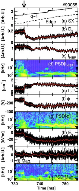
Figure 1. Time evolutions of (a) SX intensity, (b) Dα, (c) IHIBP, (d) power spectrum of IHIBP, (e)
, (f) φ, (g) power spectrum of φ, (h) Er, (i) magnetics and (j) power spectrum of magnetics.
Download figure:
Standard image High-resolution imageThe coherent oscillation at the frequency of f ≡ fELM = 1–2 kHz is observed from t ∼ 739 ms, on the all measured variables except for the magnetics. Therefore, this oscillation observed here, which we call tiny ELM in the H-mode, is not an MHD activity. The tiny ELM is triggered when the Dα signal goes below a threshold value. The poloidal mode number of the tiny ELM is deduced to be zero because the phase difference of φ is almost zero when the measurement points of the HIBP channels are aligned on the identical magnetic surface at r − a ∼ −1 cm.
Radial profiles of the turbulence amplitude in density |ñ/
 | ∼ |ĨHIBP/
 HIBP| and potential signal
, and the mean radial electric field Er are shown in figures 2(a)–(c), respectively, for the L- and H-mode plasmas. Here, tilde and bar indicate the fluctuation component and the long time averaged value of the quantity. In the H-mode, a deep electric field well Er ∼ 20 kV m−1 is formed at the edge transport barrier. Turbulence components in both the density and potential are suppressed by the transport barrier. Outside the radius of the electric field minimum at r − a ∼ −1 cm, especially around the separatrix, the fluctuation power of the potential rises up to three times larger than that at r − a < −1 cm. Figures 2(d)–(f) show frequency power spectra of density, potential and magnetics, respectively, measured at r − a ∼ −1 cm. After the L-H transition, reduction of the fluctuation power in the high frequency component in the range of 10 < f < 100 kHz is clearly observed in the density and potential fluctuations. On the contrary, the high frequency component in the magnetic field fluctuation shows the slight increase after the transition. This observation possibly implies the qualitative variation in the turbulence state before and after the L-H transition, e.g. from electrostatic turbulence to electromagnetic turbulence.
HIBP| and potential signal
, and the mean radial electric field Er are shown in figures 2(a)–(c), respectively, for the L- and H-mode plasmas. Here, tilde and bar indicate the fluctuation component and the long time averaged value of the quantity. In the H-mode, a deep electric field well Er ∼ 20 kV m−1 is formed at the edge transport barrier. Turbulence components in both the density and potential are suppressed by the transport barrier. Outside the radius of the electric field minimum at r − a ∼ −1 cm, especially around the separatrix, the fluctuation power of the potential rises up to three times larger than that at r − a < −1 cm. Figures 2(d)–(f) show frequency power spectra of density, potential and magnetics, respectively, measured at r − a ∼ −1 cm. After the L-H transition, reduction of the fluctuation power in the high frequency component in the range of 10 < f < 100 kHz is clearly observed in the density and potential fluctuations. On the contrary, the high frequency component in the magnetic field fluctuation shows the slight increase after the transition. This observation possibly implies the qualitative variation in the turbulence state before and after the L-H transition, e.g. from electrostatic turbulence to electromagnetic turbulence.

Figure 2. Radial profiles of (a) |ñ/
|, (b)
and (c) Er, and frequency power spectral densities of (d) |ñ/
|, (e)
and (f) magnetic field fluctuation, for the intervals in the L-mode and H-mode. Average is taken for 10 ms in each period. Dashed lines in (a) and (b) show noise induced error components for turbulence measurement.
Download figure:
Standard image High-resolution imageFigure 3 shows the spatiotemporal evolutions of mean
 and
signals during the L-H transition. Figures 3(a) and (b) show time evolutions of Dα and soft x-ray (SX) intensity for #90048, and figures 3(c)–(e) are constructed using 5 different discharges, in which the measurement location of the HIBP is scanned. The time axis in figures 3(c)–(e) is normalized as (t − tLH)/ΔtLH, where tLH and ΔtLH show the beginning time and typical duration of the L-H transition, respectively, and are evaluated from the Dα signal. The 5 discharges used here have a similar time evolution of Dα with a typical value of ΔtLH ∼ 1 ms. An ambiguity in determining tLH in a discharge is less than ∼100 µs. Note that ΔtLH does not have to be the actual temporal scale of the transition of electric field and/or turbulence intensity because the Dα emission is a passive signal of plasma transport. At the transition, the sawtooth crash event is routinely observed. The strong electric field well is formed at r − a ∼ −1 cm, where the full width of half maximum (FWHM) is ∼7 mm. This is comparable to the case in JT-60U, where the FWHM is ∼1 cm [20].
and
signals during the L-H transition. Figures 3(a) and (b) show time evolutions of Dα and soft x-ray (SX) intensity for #90048, and figures 3(c)–(e) are constructed using 5 different discharges, in which the measurement location of the HIBP is scanned. The time axis in figures 3(c)–(e) is normalized as (t − tLH)/ΔtLH, where tLH and ΔtLH show the beginning time and typical duration of the L-H transition, respectively, and are evaluated from the Dα signal. The 5 discharges used here have a similar time evolution of Dα with a typical value of ΔtLH ∼ 1 ms. An ambiguity in determining tLH in a discharge is less than ∼100 µs. Note that ΔtLH does not have to be the actual temporal scale of the transition of electric field and/or turbulence intensity because the Dα emission is a passive signal of plasma transport. At the transition, the sawtooth crash event is routinely observed. The strong electric field well is formed at r − a ∼ −1 cm, where the full width of half maximum (FWHM) is ∼7 mm. This is comparable to the case in JT-60U, where the FWHM is ∼1 cm [20].
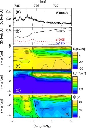
Figure 3. Time evolutions of (a) Dα and (b) SX signals for #90048, and spatiotemporal evolutions of mean (c) Er, (d)
and (e)
signals. Figures (c)–(e) are composed using 5 different discharges, in which the measurement location of the HIBP is scanned (shown by the vertical axes). Measurement location approximately corresponds to 0.85 ⩽ ρ ⩽ 1. The time axis is normalized as (t − tLH)/ΔtLH, where tLH and ΔtLH show the beginning time and typical duration of the L-H transition, respectively.
Download figure:
Standard image High-resolution imageAlthough the transport barrier is generated at a limited region in the plasma edge, a global and rapid improvement of confinement is observed just after the transition in many tokamaks. In the previous work [13], a dynamic turbulence front propagation toward the core was identified in the LCO, which can be a clue of the nonlocal improvement of confinement [33]. This front propagation is also seen during the L-H transition. In figure 3(e), the rapid propagation of the turbulence suppression front is clearly shown with the eye-guide. The turbulence suppression front starts from the edge region where the transport barrier is created, and propagates toward the core with ∼400 m s−1. To the best of authors' knowledge, this may be the first observation of the turbulence suppression front propagation during the L-H transition. In the LCO phase, there are similar observations showing the spatial propagation of the turbulence front and the electric field [8], and that of the turbulence front and the density gradient [13]. The former work addresses the long-distance propagation of the turbulence front accompanied by the electric field perturbation and/or its shear. In contrast, the latter case and the present observation show the front propagation of the turbulence suppression induced by the edge-localized electric field. Apart from the edge, the turbulence front propagation is found not to be coincident with the electric field propagation, at the present diagnostic accuracy. In any case, these observations are crucial to explore the plasma non-locality along with the theoretical prediction [34].
In order to discuss the transition mechanism, time evolution of mean quantities at the barrier location is focused on. Figure 4 shows the transition sequence at 1 cm inside the separatrix. Time evolution of the radial current is evaluated as Jr = − 0 ⊥∂Er/∂t, where 0 and ⊥ indicate the dielectric constant for vacuum and the relative dielectric constant of toroidal plasma, respectively [35, 36]. Non-ambipolar radial particle flux of electrons and ions, i.e. finite radial current, can excite Jr × B force in the poloidal direction, which drives poloidal flow structure. Even with a transient rise of the current, the confinement state can be kicked from L- to H-mode [2]. Identification of the origin of the non-ambipolar radial current is essential to understand the mechanism of the L-H transition. There are several theories that discuss the radial electric field, as has been summarized in a review article [35]. The synchronous change of mean gradient and electric field suggests the important role of the driving mechanism through neoclassical viscosity. However, this drive by neoclassical process is in proportion to the difference between the electric field and mean gradient (as is shown in [35, 37]), so that it is not at all self-evident whether this process is dominant over other mechanisms during the process of onset of transition. In further studies, this observation of the radial current will be useful in evaluating the radial current excitation mechanisms, e.g. the neoclassical flux, loss cone loss, and Reynolds stress, along with the experimental parameter using these models. Lissajous diagrams among several variables are shown in figure 5. Dual peaks in the Jr–Er Lissajous diagram are clearly shown in figure 5(b), which suggests that two different electric field excitation mechanisms co-exists. At the first transition step, an abrupt increase of the edge Er with O(100 µs) leads to increase of
(and probably the temperature gradient as well) and reduction of
. The temporal scale of transition is consistent with that estimated with electric field bifurcation theory [2, 23], including the neoclassical enhancement factor of the plasma rotational inertia, 1 + 2q2 (in the plateau regime), due to toroidal geometry [35]. No substantial change of
is seen before the change of Er. The electric field driven by the turbulence can be evaluated by the gradient of the Reynolds stress, as
0 ⊥∂Er/∂t, where 0 and ⊥ indicate the dielectric constant for vacuum and the relative dielectric constant of toroidal plasma, respectively [35, 36]. Non-ambipolar radial particle flux of electrons and ions, i.e. finite radial current, can excite Jr × B force in the poloidal direction, which drives poloidal flow structure. Even with a transient rise of the current, the confinement state can be kicked from L- to H-mode [2]. Identification of the origin of the non-ambipolar radial current is essential to understand the mechanism of the L-H transition. There are several theories that discuss the radial electric field, as has been summarized in a review article [35]. The synchronous change of mean gradient and electric field suggests the important role of the driving mechanism through neoclassical viscosity. However, this drive by neoclassical process is in proportion to the difference between the electric field and mean gradient (as is shown in [35, 37]), so that it is not at all self-evident whether this process is dominant over other mechanisms during the process of onset of transition. In further studies, this observation of the radial current will be useful in evaluating the radial current excitation mechanisms, e.g. the neoclassical flux, loss cone loss, and Reynolds stress, along with the experimental parameter using these models. Lissajous diagrams among several variables are shown in figure 5. Dual peaks in the Jr–Er Lissajous diagram are clearly shown in figure 5(b), which suggests that two different electric field excitation mechanisms co-exists. At the first transition step, an abrupt increase of the edge Er with O(100 µs) leads to increase of
(and probably the temperature gradient as well) and reduction of
. The temporal scale of transition is consistent with that estimated with electric field bifurcation theory [2, 23], including the neoclassical enhancement factor of the plasma rotational inertia, 1 + 2q2 (in the plateau regime), due to toroidal geometry [35]. No substantial change of
is seen before the change of Er. The electric field driven by the turbulence can be evaluated by the gradient of the Reynolds stress, as
 , where kr and kθ denote radial and poloidal wavenumbers of the turbulence. The observation implies the small role of the Reynolds stress in the electric field excitation, as was the case in the LCO [13]. At the moment,
and Er change simultaneously, as shown in figures 4(a) and (c), showing turbulence suppression due to the E × B shearing. In this series of discharges, the first step transition is always accompanied by the sawtooth crash event as shown in figure 5(a). The radial current peaking and the reach of the heat pulse induced by the sawtooth crash, as well as the turbulence suppression, occur at the same instant, within the present diagnostic accuracy. The impact of the heat pulse might play a role to induce a bifurcation, but, so far, no clear 'agent' associated with sawtooth has not been identified. After a short time delay (∼100 µs), the density gradient increases. In the second transition step, no SX signal peaking and little turbulence suppression are recorded. On the contrary to the first transition, the radial current is induced without a sawtooth event. Relatively slower and larger transition, compared to the first transition, in the electric field and the density gradient is clearly observed. The physical mechanism of the second step transition is still unsolved, and the clarification will be a future work.
, where kr and kθ denote radial and poloidal wavenumbers of the turbulence. The observation implies the small role of the Reynolds stress in the electric field excitation, as was the case in the LCO [13]. At the moment,
and Er change simultaneously, as shown in figures 4(a) and (c), showing turbulence suppression due to the E × B shearing. In this series of discharges, the first step transition is always accompanied by the sawtooth crash event as shown in figure 5(a). The radial current peaking and the reach of the heat pulse induced by the sawtooth crash, as well as the turbulence suppression, occur at the same instant, within the present diagnostic accuracy. The impact of the heat pulse might play a role to induce a bifurcation, but, so far, no clear 'agent' associated with sawtooth has not been identified. After a short time delay (∼100 µs), the density gradient increases. In the second transition step, no SX signal peaking and little turbulence suppression are recorded. On the contrary to the first transition, the radial current is induced without a sawtooth event. Relatively slower and larger transition, compared to the first transition, in the electric field and the density gradient is clearly observed. The physical mechanism of the second step transition is still unsolved, and the clarification will be a future work.

Figure 4. Time evolutions of (a) Er, (b)
, (c)
, (d) Jr and (e) SX signal at ρ ∼ 0.95 (r − a ∼ 1.7 cm). Dual stage is defined by the two distinguishable peaks seen in the time evolution of the radial current. Curves in t > tLH(t < tLH) are plotted with solid (dashed) trajectory.
Download figure:
Standard image High-resolution image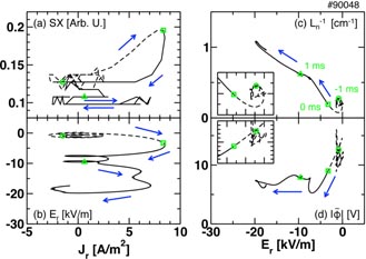
Figure 5. Lissajous diagrams in (a) Jr–SX signal at ρ ∼ 0.95, (b) Jr–Er, (c) Er– and (d) Er–. Zoomed figures at t − tLH ∼ 0 are shown inside the panels (c) and (d). Time labels are shown with open circles (t − tLH = −1 ms), squares (t − tLH = 0 ms) and triangles (t − tLH = 1 ms), in addition to the line type (curves with t > tLH(t < tLH) correspond to solid (dashed) lines).
Download figure:
Standard image High-resolution image4. Self-sustained edge transport barrier fluctuation
On the experimental study of the tiny ELM, a modulation of turbulence intensity, which might be related to the transport modulation seen in the Dα emission, is frequently discussed to determine physical mechanism that controls the continuous oscillation of the confinement with the ELM. In the present experiment, the turbulence modulation at r − a < −1 cm is not observable in the tiny ELM system, since the turbulence is already suppressed inside the transport barrier in the H-mode. The turbulence modulation seems to be localized outside the edge pedestal region, i.e. at r − a > −0.5 cm. Unfortunately, the signal to noise ratio for the turbulence intensity is too poor to discuss the phase of the turbulence components in detail even in the region r − a > −1 cm. Therefore, we avoid further discussion about the turbulence intensity modulation at present.
Figure 6(a) shows the typical waveform of the Dα oscillation in the tiny ELM sequence. The waveform is sawtooth-like that has the sharp rise and slow fall, with the amplitude of the oscillation of ∼20%. The tiny ELM activity is also seen in the envelope of the high frequency component of the magnetics (figure 6(b)), as well as other quantities measured with the HIBP. Figures 6(c) and (d) are conditional averages of the Dα signal and envelope of the magnetics with respect to the tiny ELM period. Here, the conditional average for an arbitrary function x(t) is defined as
 , where the value ti indicates the ith time instant in which the phase of the tiny ELM in Dα emission passes zero, and N is the total number of the zero passages. In the experiment, typically N = 10–20 of ensembles can be used. The phase evolution of Dα emission signal is obtained with wavelet transform. The new time variable τ takes values in −Tb < τ < Tb, where Tb is the period of the tiny ELM. The black solid curves in figures 6(c) and (d) indicate the conditional averaged signals for a single discharge #90055, while the red dashed curves show the signal averaged over 11 different discharges. The error bars on the red curves are the standard deviation of the average with 11 ensembles. The smaller standard deviation means good reproducibility of the sawtooth-like wave form at the constant amplitude. Note that the low frequency oscillation in the envelope of the high frequency component of the magnetic fluctuation is not regarded to be an activity concerning to precursors of the ELM. In many experimental devices, it is reported that the precursor of ELMs have a coherent frequency peak and a certain mode number [25]. In our case, the high frequency magnetic field is more like turbulence (see figure 3(f)), therefore the oscillation in the envelope seems to be the modulation in the broadband turbulence intensity.
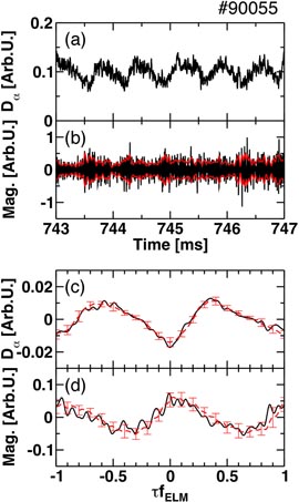
Figure 6. Evolutions of (a) Dα and (b) magnetics, and conditional average of (c) Dα and (d) envelope of magnetics for the tiny ELM period. τ is the time variable for the conditional average, where τfELM = 0 corresponds to the minimal Dα emission.
Download figure:
Standard image High-resolution imageSpatiotemporal structures of the conditional averaged
and Er are shown in figure 7. Figures 7(b) and (d) show time slices at τ fELM = −0.5 (Dα is at the top) and 0 (Dα is at the bottom) for
and Er, respectively. Strong tiny ELM activities in both
and Er are localized in the region r − a > −2 cm. When the out flux associated with Dα emission is the minimum value (τ fELM = 0), the density gradient and the radial electric field take the maximum value, and vice versa. In addition, the electric field well position clearly exhibits reciprocating motion with the characterized width of ∼1 mm. The phase profile of the φ oscillation is almost constant in space, providing kr = 0. Therefore, the oscillation is attributed to mean flow modulation, where no zonal flows are involved. The electric field oscillation is associated with the gradient of the amplitude in φ oscillation at −1 cm < r − a < 0 cm, i.e. the imaginary part of the radial wavenumber. In contrast, the amplitude in φ is almost constant at r − a < −2 cm, having only a small amplitude in Er fluctuation. The large amplitude is localized at the location of the transport barrier, r − a ∼ −1 cm. The dynamics of the tiny ELM is characterized by the periodic modulation in the strength of the transport barrier, i.e. the mean poloidal flow, the pedestal gradient, and the transport.
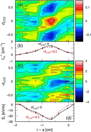
Figure 7. (a) (c) Spatiotemporal evolution of conditional averaged
[Er] and (b) (d) radial profile of
[Er] at τ fELM = −0.5 (maximal Dα) and 0 (minimal Dα).
Download figure:
Standard image High-resolution image5. Discussion
In the series of this study, we have discussed the physical mechanism of the dynamics in the LCO in the L-mode [13], the L-H transition and the tiny ELM in the H-mode. Figure 8 shows the Lissajous diagram for the three different time periods in the normalized electric field eρpEr/Ti and the normalized density gradient
 space, where ρp and Ti/e denote the poloidal Larmor radius and the ion temperature in the electron volt unit, respectively. These parameters take ρp ∼ 2 cm−1 and Ti/e ∼ 170 eV as the average values between L- and H-mode plasmas. The thin dashed curve, the red solid curve and the green solid curve show the trajectory during the L-H transition (#90055), the LCO in the L-mode and the tiny ELM in the H-mode, respectively. The phase relation seen in the tiny ELM sequence matches that in the LCO in the L-mode, which may imply the existence of the similar physical mechanism between them.

Figure 8. Lissajous diagram in eρpEr/Ti– space (Er and
are also shown). Error bars in the insert show the 95% confidence interval for the conditional average.
Download figure:
Standard image High-resolution image
Theories [2, 23] indicate that the transition to the stationary H-mode was expected with the parameters eρpEr/Ti ∼ 1 and
 . In the experiment, the critical electric field for the L-H transition has been clearly observed at eρpEr/Ti ∼ 1 in JFT-2M [18] and ASDEX-U [37]. A comprehensive picture is obtained in this experiment, as shown in figure 8. In the L-mode plasma with the input power Pin ∼ Pth (the present condition), the LCO can be turned on as the oscillatory self-regulation of the turbulence transport by the electric field and density gradient. Similar oscillation is also seen as the tiny ELM in the H-mode, at the lower frequency. These oscillations are understood as the strengthening/weakening of the transport barrier. However, they cannot kick the L-H or H-to-L transitions because of their small amplitude. Once the strong excitation of the electric field is achieved (accompanied by the sawtooth heat pulse and/or some coinciding events) and the condition eρpEr/Ti > 1 is satisfied, the L-H transition occurs. The value eρpEr/Ti > 1 is obtained only with the first transition step. The role of the second transition step, where the stronger transport barrier evolves, is still not understood, and will be addressed in future.
6. Summary
The HIBP measurement provides quantitatively clear views of the L-H transition. The main claims of the article are as follows. (i) At the L-H transition, an abrupt increase (time scale of O(100 µs)) of mean Er (which is localized in radius with FWHM ∼7 mm) leads the increase of
and the suppression of
. Reynolds stress force might remain too small to drive the abrupt increase of |Er| in the present series of observations. In the Lissajous diagram between the radial current and the radial electric field, dual peaks were found. (ii) Rapid inward propagation of the turbulence suppression front is observed at the transition. This might be linked to the fast core-edge coupling seen in global improvement of confinement after the H-mode transition. (iii) After the transition, the tiny ELM is found. Spatiotemporal dynamics of the tiny ELM are exhibited. (iv) Physical mechanism that can comprehensively explain the limit-cycle oscillation in the L-mode, the L-H transition and the tiny ELM in the H-mode is discussed. The important role of the critical electric field eρpEr/Ti ∼ 1 is confirmed.
Acknowledgments
We thank Prof P.H. Diamond, Prof G.R. Tynan, Prof U. Stroth, Prof J.-Q. Dong, Prof K.J. Zhao and Prof C. Hidalgo for useful discussions, and the late Dr H. Maeda, Prof Y. Hamada, Dr M. Mori and Dr Y. Kamada for strong support. This work was partly supported by Grants-in-Aid for Scientific Research from JSPS, Japan (21224014, 23244113, 26887047), the collaboration programs of JAEA and of the RIAM of Kyushu University and of NIFS (NIFS13KOCT001), and the Asada Science Foundation.
Footnotes
- *
This article is dedicated to the memory of Professor Tihiro Ohkawa.