


Abstract
Edge poloidal flows exceeding the poloidal sound speed lead to the formation of a pedestal structure (Guazzotto and Betti 2011 Phys. Rev. Lett. 107 125002). This result is based on the existence of 'transonic' equilibria, in which the edge region of the plasma flows supersonically with respect to the poloidal sound speed (i.e. the sound speed reduced by a factor Bθ/B), while the plasma core is rotating with subsonic poloidal velocities. The ideal-MHD equilibrium force balance shows that radial discontinuities must be present at equilibrium in the presence of transonic flows. The formation of the transonic discontinuity was proven with time-dependent simulations. In this work, we prove that the transonic discontinuity can be formed with poloidal velocities no larger than a few tens of km s−1. Such relatively slow velocities are supersonic at the bottom of the pedestal where the temperature is a few tens of eVs. We also show how realistic toroidal velocity profiles can be obtained in transonic equilibria if the appropriate choice is made for the input free functions.
Export citation and abstract BibTeX RIS
1. Introduction
The tokamak concept is a likely candidate to achieve the condition of the burning plasma state in the magnetic confinement approach. Even though great progress has been made in the last decades in tokamak experimental performance, further improvements are still required before a net power gain can be obtained from the fusion reactions in the plasma. One fundamental parameter for the plasma performance is the energy confinement time τE. A value of τE ≳ 1 s is required to achieve the burning plasma state. A way to improve τE is to reduce radial thermal transport from the plasma core. A significant reduction in thermal transport, of about a factor of 2, is observed in the so-called high-confinement mode (or H-mode) of operation, as opposed to the standard low-confinement tokamak mode of operation (or L-mode). The H-mode was discovered experimentally [1] and has been observed in all major tokamaks. The H-mode is associated with high shear in poloidal (the short way around the torus) plasma rotation. Poloidal velocity shear reduces energy transport by breaking eddies and streamers and by reducing turbulence. H-modes are also associated with a sharp radial variation of density and temperature across the region of high poloidal flow shear (density and temperature pedestals, respectively). Tokamaks spontaneously enter the H-mode of operation when a sufficient heating power is applied to the system. Notwithstanding the large theoretical effort so far invested in H-mode investigation, no conclusive explanation of the mechanism for H-mode development and pedestal formation has yet been found.
One possible physical mechanism associated with the initial phase of the formation of the flow shear and density pedestal (L–H transition) was recently proposed in [2, 3]. It was shown, with time-dependent simulations performed with the code SIM2D, that an equilibrium with initially smooth profiles for all physical quantities will naturally develop discontinuous density and velocity profiles if a source of poloidal momentum is inserted into the system. Remarkably, discontinuities develop even if the momentum source is itself smooth. In this paper, we extend the work of [2, 3] to show how it is possible to form discontinuous profiles even with relatively small velocities for the entire transient. Moreover, we turn our attention to toroidal velocity experimental measurements, and compare them with equilibrium calculations performed with the code FLOW [4], which is used to calculate steady-state discontinuous solutions (corresponding to the late-time steady-state solution of the SIM2D simulations).
The physical mechanism on which the model is based is purely geometrical, and was first introduced in [5]. It can be summarized as follows. In ideal magnetohydrodynamic (MHD), the plasma is frozen in the magnetic field lines, and therefore can only flow along field lines and not across them. Thus magnetic surfaces act as rigid walls from the point of view of the plasma. If we consider the simplest case of a low-β (β is the ratio between pressure and magnetic pressure), large aspect ratio plasma of circular cross section and look at two adjacent magnetic surfaces, we observe that a fluid element located between the magnetic surfaces will remain between the same two surfaces as it moves in the poloidal direction. If we neglect the Shafranov shift (as is legitimate for the simple case we are considering) and assume that the radial distance Δr between the two surfaces does not change along the angle, we conclude that because of toroidal geometry the cross section for the plasma flow, proportional to RΔr (where R is the torus major radius), changes with the poloidal angle, and is maximum on the outer midplane and minimum on the inner midplane. In other words, a fluid element travelling in the poloidal direction from the outer midplane will see a progressively decreasing cross section until it reaches the inner midplane and then an increasing cross section until it comes back to the outer midplane. Considering the poloidal direction as the only relevant direction, we can then analyse the properties of the flow using the well-known one-dimensional gas dynamic theory of converging–diverging deLaval nozzles (see for instance [6, p 552]). At steady state, a fluid element that starts subsonic (supersonic) on the outer midplane will see its Mach number Mp increase (decrease) until it reaches the throat of the nozzle, and decrease (increase) afterwards. The maximum (minimum) Mach number is reached at the minimum of the cross section, and can be no more than Mp = 1 for a fluid element that starts subsonic, and no less than Mp = 1 for a flow element that starts supersonic. If we now consider two fluid elements, the first just subsonic
 and the second just supersonic
 at the throat of the cross section on two adjacent magnetic surfaces, we realize that the difference
 will increase with the poloidal angle and reach a maximum at the outer midplane. The radial discontinuity in the Mach number is associated with a discontinuity in poloidal velocity, density and pressure. This is what is called the transonic discontinuity. It is important to emphasize that there is no flow across the discontinuity, and therefore no dissipation as there would be for a shock discontinuity. If a more realistic situation is considered (e.g. finite β, finite aspect ratio, arbitrary cross section) the picture becomes somewhat more complicated, but the basic physics mechanism remains valid.
In the intuitive picture of transonic equilibrium given above, we have implicitly excluded the possibility that a fluid element transitions to a different characteristic (i.e. to supersonic from subsonic flow) while travelling along the magnetic deLaval nozzle. This was done because such a transition would require an additional transition in the opposite direction (to subsonic from supersonic) before the fluid element completes a poloidal revolution. This is necessary in order to satisfy the periodic boundary condition for the flow (the velocity at θ = 2π must be the same as the velocity at θ = 0). In ideal MHD the reverse transition can only occur with a shock. A different mechanism may be involved if more detailed physics is included, but the transition can only be due to a dissipative phenomenon. What this means is that if this situation occurs in the plasma, entropy will constantly be generated, and the plasma will therefore not be in a steady state. However, the sub-supersonic transition along the direction of the flow (and its reverse) can be present during transients, when a supersonic poloidal rotation starts developing. Transients bringing the formation of transonic equilibria were first investigated with the code SIM2D in [2, 3], and will be further analysed in this work.
In the previous discussion, the poloidal Mach number Mp was introduced. This is defined as the ratio between the poloidal velocity and the characteristic plasma velocity with which information travels in the poloidal direction, i.e. the poloidal sound speed Csθ = CsBθ/B (where
 is the sound speed, Bθ the poloidal field and B the total magnetic field). Due to the fact that Bθ ≪ B in tokamaks, the poloidal sound speed is much slower than the total sound speed. Nevertheless, in [7] it was pointed out that in the core of the plasma Csθ is still much larger than measured poloidal velocities, thus excluding any relation between transonic poloidal flows and internal transport barriers. However, the plasma temperature T ∼ p/ρ is small at the edge, making the poloidal sound speed relatively small at the edge (∼10 km s−1 in the model equilibria used in our simulations), compatible with supersonic flows for velocities measured in experiments. It is worthwhile to mention that in plasma physics, in particular in astrophysics, the poloidal sound speed is more correctly identified as the poloidal magneto-slow speed. For all practical purposes the two are indistinguishable for the plasma properties examined in this paper, and we will therefore conform to the standard tokamak notation of poloidal sound speed in the rest of this work.
2. The two-dimensional MHD code SIM2D
In this section, we briefly summarize the main characteristics of the SIM2D code [2, 3], which is used for the time-dependent simulations shown in the rest of this paper. SIM2D was written to simulate transonic poloidal flows in two-dimensional MHD transients. The code is based on the resistive-MHD set of equations:


In equations (1)–(4), B is the magnetic field, V the plasma velocity, ρ the density, J the plasma current, γ the adiabatic index, η the resistivity and
 is the identity tensor. The definitions
 (total pressure) and
 (total energy) were also introduced. Here and in the following, we have set μ0 = 1 for ease of notation. The term Smom appearing on the right-hand side of equations (2) and (4) is the (input) momentum source, which is used to drive the poloidal flow in the simulations. The choice for the shape of Smom used in this paper is given later in section 3.
The code is written in Cartesian coordinates and uses a uniform, fixed, regular grid to approximate the solution of equations (1)–(4). The time stepping algorithm combines a predictor–corrector [8] scheme and an alternate-direction-implicit scheme, and is second order accurate in both time and space. A projection method [9] is used to control the
 error. Outflow boundary conditions are used for the velocity, which at the edge is assigned to be proportional to the sound speed. A mass recycling algorithm is used to prevent emptying the low-density, low-temperature halo region that surrounds the main plasma region (see figure 2 later). The edge magnetic field is assigned to be constant in time and equal to its initial (equilibrium) value. Different boundary conditions (e.g. rigid wall) were tried during the development of SIM2D. The boundary conditions mainly affect the halo region, but barely influence the main plasma. This is because the main plasma region is close to ideal; therefore the plasma is confined in the closed-field line region. Indeed, it was verified that different boundary conditions do not have a strong influence on the formation of the MHD pedestal. Standard Von Neumann–Richtmyer numerical dissipation [10, p 311] is used in the simulations. In this work, a resolution of 500 points in each direction was used. All simulation results are shown in physical units; times are normalized to the poloidal revolution time τp in the supersonic region, which is case dependent and calculated a posteriori after the rotation profile in the simulation has fully developed.
Initial conditions for the code are obtained from a high-resolution equilibrium calculated with FLOW [4]. In this work, we will only discuss SIM2D results relative to a single FLOW equilibrium, which is described in more detail in section 3. What is important to emphasize is that the starting point for the simulations is an L-mode equilibrium, in which all plasma parameters are continuous, and that the momentum source is also smooth. Thus, any discontinuity appearing in the results is not due to any special choice in the input profiles, but solely to the physical mechanism described in section 1. This is illustrated by the plots in figure 1. The figure shows the comparison of the velocity profile at time t = 0.84τp and the time integral of the velocity source (i.e. the momentum source divided by the time-dependent density) to the same time. Both curves are shown in logarithmic scale. The difference between the source profile and the velocity profile is evident. In particular, the velocity profile has a sharp gradient at R ≃ 2.25 (the transonic discontinuity), where the integrated source profile is smooth.
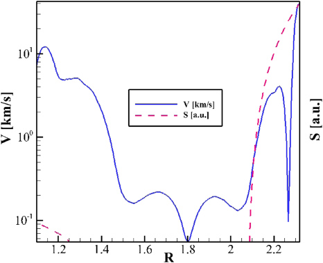
Figure 1. Comparison between poloidal velocity profile on the midplane at time t = 0.84τp (solid curve) and time integral to 0.84τp of the velocity source (dashed curve) in logarithmic scale. Notice the large velocity shear at R ≃ 2.25, and the corresponding smooth source profile.
Download figure:
Standard image
Figure 2. Initial plasma density (colourmap) and magnetic surfaces (black lines) in the simulations used in [2, 3] (left) and in the simulations in section 3 of this paper (right).
Download figure:
Standard image3. SIM2D simulations with small momentum source
After proving the possibility of generating a density pedestal and a high poloidal flow shear by introducing a smooth poloidal momentum source in the system with time-dependent simulations [2, 3], we turn our attention to the level of velocity that is required to generate the pedestal structure at the plasma edge. It is important to emphasize that the pedestal forms when the poloidal velocity at the plasma edge (i.e. at the bottom of the pedestal) is supersonic with respect to the poloidal sound speed. To investigate the issue, a new series of simulations with respect to the ones presented in previous work was ran. For convenience, we refer to the new set of simulations as the 'low-Vθ' simulations in the rest of this paper. The new simulations start from an equilibrium similar (but not identical) to the one used in [2, 3]. The geometry of the old (left) and new (right) equilibria is shown in figure 2. In the figure, solid lines represent magnetic surfaces and the colourmap corresponds to plasma density. In both equilibria, the main plasma region extends to the last magnetic surface drawn inside of the LCFS. The low-density, low-temperature external region corresponds to the halo plasma. The main difference between the old and new equilibria is the use of smoother input profiles, in order to avoid the numerical problems occurring late in time in the previous set of simulations. The main plasma parameters, summarized in table 1 are intentionally similar to the previous simulation ones, with the purpose to make a meaningful comparison between the two sets of simulations possible. The slightly smaller plasma surface in the new simulations is not particularly important. Arguably, the equilibrium parameter that has the largest influence on the maximum poloidal velocity for transonic equilibria is the edge temperature, which directly determines the poloidal sound speed,
 . In the simulations presented in this paper, Tedge = 30 eV was used. As for the momentum source used to drive the flow, we use the same profile that was used in [2, 3],
where α is a dimensional constant used to control the strength of the source and ψm is an input parameter used to set the source to zero in the core region of the plasma. The momentum source is proportional to the density, so that the velocity source (=Smom/ρ) remains smooth even after the density develops a discontinuity (see figure 1, at the time of the figure the density discontinuity has already formed in the outboard part of the plasma). Therefore the velocity discontinuity is not generated by the source shape, but by the physics of the system evolution. The source dependence on the poloidal angle θ is used to mimic a momentum source that is peaked on the outboard midplane and vanishes on the inboard side of the plasma, such as, for instance, a momentum generation due to turbulence driven by unfavourable curvature. The development of a physics-based model of the poloidal momentum source will be the subject of future work. Some details regarding future plans are given in the appendix. It is important to observe that the position of the discontinuity is determined by the source shape and strength. Since the discontinuity forms between an edge supersonic region and an inner subsonic region (always referring to the poloidal sound speed), moving inwards from the plasma edge, the discontinuity will form at the radial location where the source becomes too weak to drive the plasma to supersonic speeds. Thus, for instance increasing the source strength without changing its shape will make the discontinuity move inwards, and making the source profile narrower without altering its strength will make the location of the discontinuity move outwards.
Table 1. Main plasma parameters for the DIII-D model equilibrium.
| Parameter | Meaning | Value |
|---|---|---|
| βt | Toroidal
 |
1.15% |
| Ip | Plasma current | 670 kA |
| βp | Poloidal beta = 2〈p〉/〈Bp〉2 | 0.42 |
| R0 | Major radius | 1.69 m |
| a | Minor radius | 0.61 m |
| BV | Vacuum field | 1.26 T |
| TE | Edge temperature | 30 eV |
| TC | Temperature on axis | 3 keV |
It is worthwhile to emphasize that the size of the momentum source used in our simulations (and also in the simulations presented in previous work) is rather small as compared with the order of magnitude of the momentum dissipation due to poloidal viscosity in the system. This is due to the fact that no physical momentum dissipation mechanism is included in the system, yet. Thus, the momentum source needs to overcome only the numerical dissipation in order to make the plasma spin. Introducing a model for the poloidal viscosity in the simulations will also be the subject of future work, and it will allow us to evaluate in a more realistic way the amount of power required to drive the poloidal rotation. Some details regarding future plans for this issue are also given in the appendix. At any rate, it was shown in [3] with a scaling analysis that the amount of power required to drive edge poloidal flows is small compared with the power exhausted through the pedestal.
In principle, the only requirement for the existence of a transonic equilibrium is that the poloidal velocity must exceed the poloidal sound speed in the edge region of the plasma (i.e. at the bottom of the pedestal), i.e. at all angular locations for ψ > ψtransition. Numerical equilibrium calculations show that in the outboard region of the plasma the minimum poloidal Mach number for transonic equilibria is Mp ≃ 2–2.5. This is due to the fact that in the supersonic region the poloidal Mach number in the outboard part of the plasma must be larger than the Mach number in the inboard part, as is discussed in more detail in [5, 11]. The situation is illustrated in figure 3, showing the poloidal Mach number profile along the midplane for a DIII-D equilibrium with small edge poloidal velocity computed with FLOW. In the figure, each dot corresponds to a grid point: the discontinuity in the Mach number in the outer midplane is visible. Also, it is clear that the equilibrium Mach number is larger in the outboard region than in the inboard region for supersonic flows, and vice versa for subsonic flows.

Figure 3. Poloidal Mach number profile in a FLOW equilibrium with low edge poloidal velocity.
Download figure:
Standard imageIn principle, one could expect to find the same range of Mach numbers for time-dependent simulations. In practice, numerical limitations require slightly higher Mach numbers in our SIM2D simulations, even though maximum Mach numbers as low as the ones predicted by equilibrium theory are observed transiently (see below). This is mainly due to the fact that the velocity and Mach number profiles depend in a highly non-linear way on the input momentum source profile, so that it is not possible to directly control the profiles by requiring a minimum-velocity transient. Rather, we can only proceed by trial and error, adjusting the momentum source strength in order to keep the poloidal rotation supersonic and the maximum velocity low.
The maximum poloidal velocity in the low-Vθ simulations is shown versus time in figure 4. The figure shows that during the transient, the poloidal velocity never exceeds 45 km s−1, arguably not an unrealistic value, as compared with measured and inferred velocities in DIII-D or other tokamaks H-mode plasmas [12–14]. In contrast, the maximum poloidal velocity observed in the simulations presented in [2, 3] was almost double, and of the order of 88 km s−1. Moreover, the maximum poloidal velocity is of the order of
 for most of the transient. In the figure, three times are indicated with distinct symbols. First, a red circle marks the time when the edge poloidal velocity first becomes larger than the poloidal sound speed (this occurs in the outer midplane, where the source intensity is largest). Next, a red square shows the time when the edge poloidal velocity is supersonic at all angular location, and therefore two separate plasma regions (a subsonic core one and a supersonic edge one) are effectively present. Last, a red 'P' shows the time when the MHD pedestal (i.e. both the outer transonic pedestal and the inner pedestal due to mass redistribution) is completely formed (the definition of this time is only approximate).
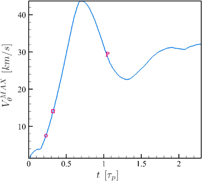
Figure 4. Maximum poloidal velocity in the system as a function of time. The red circle marks the time when the velocity first becomes supersonic in the outboard plasma region, the square the time when the edge poloidal velocity is supersonic at all angular locations, and the 'P' the time when the MHD (inner and transonic) pedestal is completely formed.
Download figure:
Standard imageAs for poloidal Mach numbers, the time evolution of the maximum Mach number in the plasma region during the transient is shown in figure 5. The Mach number shown in figure 5 is located at the outer midplane. The maximum Mach number in the computational region is actually higher than the value at the outer midplane. This is because at the X-points, which are located in the halo region, the poloidal magnetic field and hence the poloidal sound speed vanishes. Therefore, large numerical values Mp ≫ 1 are found at the X-points, even for relatively small poloidal velocities,
 . It is seen from figure 5 that the maximum Mach number in the plasma never exceeds
 , somewhat larger than the minimal required
 obtained from equilibrium calculations. Also, once the MHD pedestal is formed,
only changes slowly, and it remains around a value of
obtained from equilibrium calculations. Also, once the MHD pedestal is formed,
only changes slowly, and it remains around a value of
 , not too far from the equilibrium results. It is reasonable to expect that the formation of the MHD pedestal can occur with maximum Mach numbers (and thus velocities) even lower than the ones reported in this section. In particular, the relatively fast rotation with
 at the beginning of the transient is likely not necessary. At any rate, we consider the results of this section sufficient to define an upper limit for the range of Mach numbers required in order to generate the MHD pedestal. One should also keep in mind that the inclusion of additional physics in the simulations, in particular of neoclassical poloidal viscosity, will certainly affect the transient and its maximum velocities.
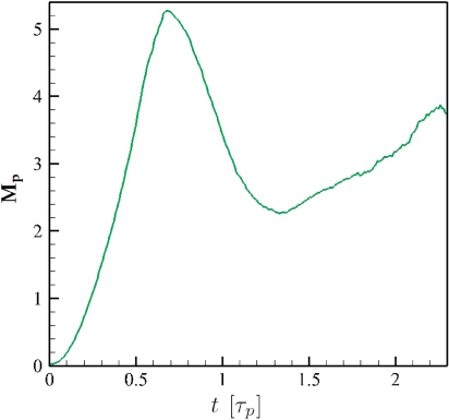
Figure 5. Maximum poloidal Mach number in the system as a function of time.
Download figure:
Standard image4. Equilibria with discontinuous input free functions
The most distinctive property of transonic equilibria is the presence of radially discontinuous profiles for all plasma properties. As discussed in [2, 3], equilibrium profiles are discontinuous at all angular locations except for the inner midplane if the input free functions are all continuous. However, conservation of mass generates a density profile with an inner pedestal, which is not due to the transonic discontinuity, but which can be reproduced in equilibrium calculations assigning a discontinuous profile for one of the five free functions of ψ that are necessary as input for transonic equilibrium calculations. In this section, we turn our attention to yet another physical quantity that was not investigated in detail in [2, 3], namely the plasma toroidal velocity Vφ. Here and in [3] the equilibrium code FLOW is used to calculate transonic equilibria. FLOW is described in detail in [4], and will not be further discussed here. In this section, we will use a DIII-D model equilibrium, similar but not identical to the one used in SIM2D simulations.
A typical profile for Vφ in a transonic equilibrium calculated with FLOW is shown by the black curve in figure 6 (the sharp variation of Vφ in the inboard region of the plasma, which is not a discontinuity, is due to the localized profile chosen for the poloidal velocity, which turns into a localized profile for φ(ψ) in equation (6)). At the transonic surface the toroidal velocity shows a finite discontinuity, which in the equilibrium in figure 6 is of the order of ΔVφ ≃ 72 km s−1. As discussed in section 5, experimental profiles of Vφ do not show large discontinuities of this size. One can easily expect that toroidal momentum transport will make such large discontinuities disappear. It is then worthwhile to investigate what is the minimum size of the toroidal velocity discontinuity that is compatible with the ideal-MHD equilibrium theory. Interestingly, it is possible to reduce the size of ΔVφ by taking into account the equilibrium definition of Vφ:

On the right-hand side of equation (6), if all input free functions are continuous, the only discontinuity is in the density ρ (strictly speaking, Bφ is also discontinuous, but ΔBφ/Bφ ≪ 1 and the discontinuity in Bφ can thus be ignored for the purpose of this discussion). It is therefore possible to modify the profile of the input free functions in such a way that the discontinuity in Vφ will be removed. In particular, it is possible to assign a jump in Ω that will compensate the jump in ρ. However, it is necessary to take into account that the toroidal field is given with excellent approximation by

Therefore it is possible to make Vφ continuous only at a single value of R, R = Rs. Writing the discontinuity in toroidal velocity at the transonic surface ψ = ψtr as

we obtain

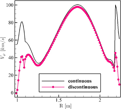
Figure 6. Toroidal velocity profile along the midplane for a FLOW equilibrium with continuous Ω(ψ) (black curve) and with discontinuous Ω(ψ) (red curve, dots).
Download figure:
Standard imageIn writing equation (9) one should also keep in mind that ρ is a function of (R, Z); so an appropriate choice must also be made for the value of Δρ to be used in the equation. Clearly, the value Rs can be chosen arbitrarily. One additional subtlety that must be taken into account is that the density profile and its jump (which needs to be obtained from an equilibrium calculation) also depend on the toroidal velocity profile (see [5]). Moreover, the value ψtr too depends in a non-trivial way on the input free functions, and is modified by introducing a discontinuity in Ω(ψ) (even though in practice the modification is small for low β plasmas with reasonable velocities). For these reasons, it is necessary to iterate on equation (9) in order to remove the toroidal velocity jump at the desired location Rs. Alternatively, if the angular location of the continuous toroidal velocity profile is not the most important parameter in the resulting equilibrium, one can assign an input value for Rs and obtain a continuous profile at a slightly different location R's ≃ Rs. This was the approach used for the equilibrium shown with the red, dotted curves in figures 6 and 7. In this case, the main purpose of the discontinuity in Ω(ψ) is to reduce the jump in Vφ to more realistic values. As seen from figure 6, this is indeed possible. More precisely, the maximum jump in Vφ in the equilibrium with continuous Ω(ψ) is of the order of ∼72 km s−1, while the jump in the equilibrium with discontinuous Vφ is reduced to ∼20 km s−1. A detailed analysis of the two-dimensional output of the equilibrium calculation (not shown) proves that the radial jump in Vφ at the outer midplane is close to the maximum radial jump in Vφ. This is not automatic, since by assigning a discontinuity in a free function one could move the position of the maximum jump in toroidal velocity to a different angular location. Coming back to figure 7, several points can be made from the comparison of the density profiles in the two equilibria. First, we observe that, notwithstanding the change in one of the input free functions, the profiles are essentially identical in most of the plasma. In particular, the transonic discontinuity for the density is not modified, even though the toroidal velocity profile is quite different at the outer midplane on the transonic surface. Notably, the poloidal velocity profile is also only marginally affected by the change in Ω(ψ) (not shown). Both equilibria are ran with a resolution of 128 × 128 points, and in figure 7 each symbol corresponds to a grid point, so that a sharp variation between two consecutive symbols corresponds to a discontinuity in the calculated profile. The only visible difference between the two profiles is the inboard side, where the profile with discontinuous Ω(ψ) has a steeper gradient near the transonic surface. In fact, high-resolution calculations (512 × 512 points) confirm that the steep gradient in the inboard side of the plasma is a veritable discontinuity, while the density profile of the equilibrium with continuous Ω(ψ) is continuous, even though steep, as expected from theory. This should not come as a complete surprise. As mentioned earlier, the density profile is modified by the choice of Ω(ψ). In particular, a discontinuous Ω(ψ) can and does result in a discontinuous density profile. This is not dissimilar from the case investigated in [3], where a discontinuous input free function is assigned in order to create a discontinuous density profile at all angular locations. More details on the equilibrium density profile are given in [5].

Figure 7. Density profile along the midplane for a FLOW equilibrium with continuous Ω(ψ) (black curve, squares) and with discontinuous Ω(ψ) (red curve, circles).
Download figure:
Standard imageIn conclusion, it was shown in this section and in [3] that the properties of transonic equilibria that are dissimilar from experimental profiles can be ameliorated by a judicious choice of the input free functions. In particular, with respect to the toroidal velocity, it was shown that the large discontinuity in toroidal velocity obtained in standard transonic equilibrium calculations can be reduced to more realistic values by assigning a discontinuous profile for the rigid toroidal rotation frequency Ω(ψ). It is interesting to observe that discontinuities exist in transonic equilibria even if all input free functions are perfectly smooth. Perhaps somewhat counterintuitively, a discontinuous input can instead be used to make equilibrium profiles 'less discontinuous'.
5. Comparison with experimental measurements
The most important test bed for any theory is the comparison with experimental findings. Transonic equilibria have several distinctive characteristics that should in principle make a comparison with experimental measurements very straightforward, thus allowing us to recognize if transonic equilibria are present in experiments. Unfortunately however, the most important plasma properties of transonic equilibria are the ones that are hardest to measure in experiments. In particular, the measurement of sharp gradient and a high level of poloidal rotation at the plasma edge, with its two-dimensional structure, is beyond the capabilities of present diagnostics. Some 'coarser' properties, such as the transonic dip (a minimum in poloidal velocity just inside the pedestal) appear to be present in experiments (see for instance figure 9 in [14]), but they hardly constitute a final proof of the presence of transonic equilibria in experiments. The two-dimensional structure of the density just after the L–H transition is also not easily available from experimental data.
In light of the discussion in section 4, in this paper we turn our attention to the toroidal velocity profile. Toroidal flows are much better diagnosed in experiments than poloidal flows: if discontinuities of the order of the ones predicted by transonic equilibria are found in experiments during the (early) H-mode phase, this would constitute at least a good hint of the relevance of transonic equilibria to H-mode plasmas. Before proceeding with the analysis, it is important to recall that the ideal-MHD transonic pedestal has zero width for the sharp variations at the transonic surface. In experiments, the pedestal has a finite width (typically ∼ 1 to a few centimetre), which is determined by physics that is not included in the ideal-MHD model. When considering experimental measurements, we will compare the size of the discontinuities predicted by the theory with the size of the sharp variations measured across the pedestal. Since the numerical work presented in the previous part of this paper referred to the DIII-D tokamak, and since DIII-D has excellent diagnostics for toroidal flows, we will mainly consider DIII-D measurements in this section, and only make some brief reference to other experiments. Needless to say, the literature on toroidal flow measurements is quite extensive. In the following, we will only consider a few meaningful samples and compare them with our numerical results.
As discussed in section 4, we expect radial transport of toroidal momentum to quickly minimize toroidal flow discontinuities after the formation of the MHD pedestal. Since momentum transport is not included in SIM2D simulations, and since the reduction of the toroidal flow discontinuity, although quick, will happen on time scales longer than the time scales covered by SIM2D simulations, it is not meaningful to compare SIM2D toroidal velocity profiles with experimental profiles. Rather, we consider the results of the equilibrium calculations in section 4 for our comparison with experimental measurements.
For our purpose, the most interesting results for toroidal velocity measurements in DIII-D H-mode plasmas are reported in [15, 16]. In these references, a Langmuir probe situated 18.8 cm under the midplane is used to measure the toroidal velocity in the region at the bottom of the H-mode pedestal under various plasma conditions (co- and counter-injection for NBIs, ECH heating). Impurity velocity is used as a proxy for main ion velocity in the core of the plasma. Several remarkable points can be made from the results shown in [15, 16]. First, it is seen that the toroidal velocity peaks inside the LCFS. Moreover, there is no appreciable velocity peak before the L–H transition. Finally, the toroidal velocity variations over a small radial distance (∼1 cm) are of the order of ∼10 to a few tens of km s−1 under all plasma conditions, roughly compatible with our numerical results in section 4.
More puzzling, but still at least partially supportive of the results of theory are the measurements shown in [17]. In this work, a one-dimensional theoretical model is used to calculate several properties of the plasma, with a set of experimental measurements as input. Without getting into the details of the model, we just comment on the resulting calculated main ion velocities. Of the three H-mode shots analysed in the paper, two show fairly smooth profiles for poloidal and toroidal velocity, while one has a quite large main ion poloidal velocity (∼60 km s−1 at the edge), and a fairly large and sharp variation of Vφ near the edge (∼25 km s−1), once again compatible with the results of equilibrium calculations.
Some interesting results can be found also for other experiments. For instance, we can consider [18] for JET. In that work, a spectroscopic diagnostic is used to measure the rotation velocity of impurities. It is found that there is a sharp velocity transition at the edge, of the order of ∼30 km s−1. In truth, a similar sharp transition seems to be present in both the L- and H-mode. However, what seems most important for the purpose of this paper is that there is a measured jump in toroidal velocity of the order of tens of km s−1, again at least in qualitative agreement with the theoretical results presented in section 4.
Sharp variations of the toroidal velocity are also observed in a completely different machine, the spherical torus MAST. In [19] edge toroidal velocity measurements obtained using a gas puffing diagnostic are shown. In H-mode plasmas, sharp variations of the toroidal velocity, of the order of ∼5–10 km s−1 are observed at the edge. This is somewhat smaller than what is obtained in regular tokamaks, and than what is predicted for DIII-D by transonic equilibrium calculations. More analysis on low-aspect ratio plasmas will be required to evaluate the properties of transonic equilibria with discontinuous input free functions.
6. Conclusions
This work is based on the model for transonic equilibrium that was first proposed in [5] and solved numerically in [4], and on its possible connection with the early phase of the L–H transition, which was suggested in [2, 3]. The two main results of this paper are as follows. First, it was shown that the MHD pedestal can be formed with relatively low Mach numbers during the entire transient,
 , and Mp < 2–4 in the whole plasma during most of the transient. Granted that these results are not a conclusive proof of the relevance of transonic equilibria to tokamak experiments, they do go in the direction of showing that transonic equilibria do not require inordinately large poloidal velocities to exist. This occurs because the supersonic flow is localized at the bottom of the pedestal, where the poloidal sound speed is rather low. The second main result of this paper is the calculation of transonic equilibria with realistic toroidal velocity discontinuities. Equilibrium results predict that all plasma properties are discontinuous if the poloidal rotation is transonic. In particular, large radial jumps in toroidal velocity are expected, much larger than poloidal velocity jumps, and also likely larger than what is observed in experiments. It was shown in section 4 that it is possible to significantly reduce the size of the toroidal velocity discontinuity by choosing a discontinuous profile for one of the input free functions of the equilibrium, namely the rigid toroidal rotation Ω(ψ). With the appropriate size and position of the discontinuity in the input, the resulting equilibrium profile for Vφ has a much smaller jump than the one obtained with a continuous input (∼20 km s−1 versus ∼72 km s−1 for the model DIII-D equilibrium used in the calculations). It was then shown in section 5 that the toroidal velocity discontinuity obtained in the previous section is in fact compatible with experimental measurements. In experiments, toroidal velocity variations of the order of a few tens of km s−1 across the pedestal region are routinely measured in H-mode plasmas. Clearly, these results again do not constitute a conclusive proof of the relevance of transonic equilibria to tokamak H-modes, but they certainly prove that realistic toroidal velocities can be obtained in transonic equilibrium calculations.
Acknowledgments
This work was supported by DOE under grant DE-FG02-93ER54215. Participation to the 2011 H-mode workshop of one of the authors (LG) was made possible by Marie Curie Grant PIRG-GA-2009-256385.
Appendix.: Future plans for model physics improvement
A physics-based momentum source and neoclassical poloidal viscosity will be implemented in SIM2D in the near future. First, the generation of poloidal flow due to ion-orbit losses will be considered [20]. Ions are lost near the edge due to finite banana width. The charge imbalance caused by the ion loss causes a radial electric field, which in turn produces a poloidal rotation. An explicit expression for the momentum source is given in [20] in terms of collisionality, geometry and orbit shape, and will be implemented in the code:
 , where angular brackets indicate flux surface averages,
 is the poloidal viscosity term (expressed in terms of surface integrals, plasma velocity and collisionality in [20]), M is the ion mass, N the plasma density, Γorbit the particle flux associated with the ion-orbit loss and c is the speed of light. The work in [20] is based on the solution of the drift-kinetic equation with mass flow velocity. Another source of poloidal rotation is the momentum deposition due to auxiliary heating, either neutral beam injection (NBI) [21] or radio-frequency (RF) heating [22]. Neutral beams deposit momentum in the plasma through collisions. A detailed kinetic model of the beam attenuation is contained in [21], where the fast-ion population evolution is calculated using a Monte Carlo method. SIM2D can be coupled to the NUBEAM code to calculate the effect of NBI on the plasma properties (both temperature and rotation). However, at least the first implementation will rely on a simplified attenuation (and momentum deposition) model for the beam. Momentum deposition from RF heating is similar to the mechanism of spontaneous flow generation from ion loss. Since energy is deposited only at specific resonance locations, RF heating causes a symmetry break between the inward and outward drifting parts of a banana orbit, producing a net non-ambipolar radial drift. The radial drift produces a charge separation and, therefore, a radial electric field. An approximate explicit expression for the radial electric field is given in [22].
Regarding neoclassical poloidal viscosity, detailed kinetic calculations for neoclassical fluxes are beyond the scope of our planned work. The implementation will instead rely on analytical approximations of the poloidal viscosity. For instance, (a simplified version of) the analytic expressions contained in [23] could be implemented. In [23] the poloidal viscosity on each magnetic surface is expressed in terms of flux averages of macroscopic quantities. A rigorous treatment will require a considerable computational effort, due to the bookkeeping necessary to keep track of the poloidal magnetic flux and, at least in principle, to the large number of flux averages to be calculated, since grid points are distributed on a Cartesian grid rather than on flux surfaces. The implementation of the poloidal viscosity will, at least initially, rely on further approximations; e.g. the use of a fixed small number of magnetic surfaces and one-dimensional interpolation for mitigating the computational requirements.