Memristor-based neural networks

Andy Thomas

doi:10.1088/0022-3727/46/9/093001

1. Introduction

If we follow Chua's original line of argumentation in his seminal paper in which he introduced the memristor, we find the following concept [1]. There are four fundamental circuit variables, namely, the charge (q), voltage (v), current (i) and flux linkage (φ). Consequently, there are six two-variable combinations of those four elements. Two of these combinations are defined by $q(t) = \int^t_{-\infty} \rmi(\tau)\,\rmd\tau$ and $\varphi(t) = \int^t_{-\infty} v(\tau)\,\rmd \tau$ .

Three more relationships are given by the resistor (combining i and v), capacitor (q, v) and inductor (φ, i) (figure 1). Consequently, Chua wrote [1] From the logical as well as axiomatic points of view, it is necessary for the sake of completeness to postulate the existence of a fourth basic two-terminal circuit element which is characterized by a φ–q curve [footnote]. This element will henceforth be called the memristor because, as will be shown later, it behaves somewhat like a nonlinear resistor with memory.

Now, we will consider a general definition of discrete memory elements that have time-dependent and non-linear responses. We follow the definitions provided by Di Ventra et al [2, 3]. Let u(t) and y(t) be the input and output variables of a system, respectively. u and y are the complementary constitutive circuit variables, such as the current, charge, voltage and flux. Subsequently, an nth-order, u-controlled memory element can be defined by

$\begin{equation*} y(t) = g(x,u,t)u(t) \end{equation*}$

$\begin{equation} \frac{\rmd}{\rmd t}x = f(x,u,t), \end{equation} \tag{ 1 }$

where x is an n-dimensional vector of the internal state variables, g is the generalized response, and f is a continuous n-dimensional vector function. For a memristive system, equation (1) becomes

$\begin{equation*} V_M(t) = R(x,I,t)I(t) \end{equation*}$

$\begin{equation} \frac{\rmd}{\rmd t}x = f(x,I,t) \end{equation} \tag{ 2 }$

where V_M and I indicate the voltage across and current through the device, respectively, and R denotes the memristance [4]. Again, from a symmetry point of view, we can introduce a meminductive and a memcapacitive system in a similar manner using flux-current and charge–voltage pairs, respectively [2, 3]. However, meminductive and memcapacitive systems are not further discussed in this paper. For a good introduction and an even further generalization of equation (1), please refer to Pershin and Di Ventra [5]. Strictly speaking, a memristor is an ideal memristive system and we tried to distinguish between the two in this paper.

In the late 1990s, researchers from Hewlett-Packard Laboratories and the University of California (Los Angeles) were studying electronically configurable molecular-based logic gates [6]. The concept was further refined by Snider et al (HP Labs) when they presented a CMOS-like logic in defective, nanoscale crossbars in 2004 [7], computing with hysteretic resistor crossbars in 2005 [8] and self-organized computation with unreliable, memristive [sic] nanodevices in 2007 [9].

A basic form of a memristive device consists of a junction that can be switched from a low- to a high-resistive state and vice versa. This behaviour can be accomplished with a simple switch. The switch closes above a threshold voltage, opens below a second threshold voltage, and the device breaks well beyond either of the threshold voltages. The nano-switches can be deposited by, e.g., electron-beam evaporation or sputtering and more than 10¹⁰ switching cycles were shown for some of the layer stacks [10, 11]. A memristor usually exhibits a characteristic, pinched hysteresis loop which is illustrated in figure 2.

**Figure 2.** An idealized iv-curve of a memristive system subjected to a periodic voltage V = V₀ sin(ωt). The result is a characteristic, pinched hysteresis curve.
Download figure:
Standard image

In 2008, researchers from HP-labs combined the interest in the younger field of nano-ionics [12, 13] with Chua's concept. They reused the term memristor (although for a memristive system), presented an experimental realization, and created a new research field that resulted in more than 120 publications about memristors and memristive systems by 2011 [14].

A straightforward way to consider a memristor is as a potentiometer, i.e. an adjustable resistor. Every time a certain amount of flux (V s) flows in one direction through the device, the resistance increases. If the current flows in the other direction, the resistance decreases. In an ideal memristor, a pulse that is half the voltage and twice the duration will result in the same change in resistance, because the resistance depends on the flux. This effect is evident in figure 3, which shows one of our memristive tunnel junctions as an example (see [15]). The curvature of the plot is an indication that it is helpful to distinguish between memristive systems and (ideal) memristors.

**Figure 3.** Total change in the resistance of a memristive system depending on the flux. The resistance continuously decreases with increasing flux.
Download figure:
Standard image

The growing interest in memristors has resulted in the development of several concepts for the use of these devices, such as utilizing memristive systems for (reconfigurable) logic circuits [16–20], or new computer memory concepts [21–23]. The simulation of memristive behaviour in electric circuits is also possible [24–28].

However, one of the most promising applications for memristors is the emulation of synaptic behaviour. Here, we will investigate memristor-based neural networks with a focus on systems that are inspired by biological processes. For this investigation, we first introduce mechanisms for the biological neural networks, e.g., in the brain. The presented processes have been identified over the past decades to be crucial for learning and memory and were initiated by Hebbs influential work, The Organization of Behavior [29]. These mechanisms will be presented in the following section. Then, we will review experiments, and mostly disregard simulations [30–33] that use memristive systems to realize the same processes.

2. Biological mechanisms

In this section, we will introduce the basic components of biological neural networks and their primary features. We begin with the schematic of two interconnected neurons, which is shown in figure 4.

**Figure 4.** Schematic representation of two interconnected neurons. The contact areas where the information is transmitted are called synapses. A signal from the presynaptic cell is transmitted through the synapses to the postsynaptic cell.
Download figure:
Standard image

A neuron interacts with a second neuron through an axon terminal, which is connected via synapses to dendrites on the second neuron. The information is transported by changes in membrane potentials, which can be generated by the influx of positive ions, such as Na⁺. The information flow transported by the membrane potentials is directed from the presynaptic to the postsynaptic cell. A central concept in biology is the plasticity of synaptic junctions. Eccles and McIntyre wrote [34] Plasticity in the central nervous system, that is, the ability of individual synaptic junctions to respond to use and disuse by appropriate changes in transmissive efficacy, is frequently postulated or implied in the discussions on the mechanisms underlying the phenomena of learning and memory [35, 36]. Therefore, we are interested in mimicking this plasticity with an artificial device.

However, achieving a one-to-one relationship between an artificial device and natural neuron connections is a very challenging task. Hyman and Nestler reported [37] that every neuron is usually connected via thousand, sometimes more than several thousand, synapses with other neurons. [...] neurons may release more than one neurotransmitter at any given synapse, adding yet another layer of complexity. Fortunately, exactly imitating nature (i.e. connecting a neuron to a second one via many synapses) is not necessary to mimic the functionality of the neural network. For the moment, we assume a net transmissive efficacy between two neurons that is mediated by the sum of the net synapses and call this efficacy the (global) plasticity of the connection. This process is illustrated in figure 5, which is a further simplification of the two neurons depicted in figure 4. For more information on the interconnection of neurons please see, e.g., Deuchars or Daumas et al [38, 39]. The neurons can interact via excitatory and inhibitory synapses. Curtis and Eccles described how the excitatory and inhibitory synaptic potentials can be integrated within a neuron [40]. This process is further explained in the integrate-and-fire section, in short, signals through excitatory and inhibitory synapses increase and decrease the possibility of the neuron to fire, respectively.

**Figure 5.** Further simplified, schematic representation of two interconnected neurons. The connection between the neurons is mediated through a single synapse with a net transmissive efficacy that represents the net connection strength of the several synapses (three in the case of figure 4) in a biological neuron connection.
Download figure:
Standard image

There are several different properties of a neuron that can be emulated by artificial devices, and some of these properties are crucial in an artificial neural network. We will discuss these mechanisms in the following few paragraphs.

2.1. Long-term potentiation

An important mechanism in biological neural networks is long-term potentiation (LTP) that has [since] been found in all excitatory pathways in the hippocampus, as well as in several other regions of the brain, and there is growing evidence that it underlies at least certain forms of memory [41, 42], as indicated by Bliss and Collingridge [43]. LTP designates a long-lasting change in the plasticity of a connection and is defined by the same authors in the following way [43]: Brief trains of high-frequency stimulation to monosynaptic excitatory pathways in the hippocampus cause an abrupt and sustained increase in the efficiency of synaptic transmission. This effect, first described in detail 1973 [44, 45], is called long-term potentiation (LTP). An example is shown in figure 6.

**Figure 6.** An example of LTP. A large stimulus that was delivered after one hour triggered a long-lasting response. Adapted by permission from [43], copyright (1993).
Download figure:
Standard image

Bliss and Collingridge also reported that LTP is characterized by three basic properties: cooperativity, associativity and input-specificity [43]. We will discuss these three characteristics in the following paragraphs.

Cooperativity means that there is an intensity threshold to induce LTP, and this threshold is above the stimulus threshold that leads to a minimal synaptic response [46]. This process is illustrated in figure 7. A small-intensity stimulus was used in figure 7(a). While there is a reaction, the potentiation disappeared approximately 5 min after application of the stimulus. This behaviour changes if a stimulus of higher intensity is used (figure 7(b)). The potentiation lasts a longer time, although the initial potentiation is of comparable size. The stimulation in a biological system is usually a tetanus, i.e. rapidly repeated impulses. Therefore, the threshold for inducing LTP is a complex [complicated] function of the intensity and pattern of the tetanic stimulation ([43]). This concept is discussed in more detail by [47].

**Figure 7.** A low- (a) and high-intensity stimulus (b) was applied to a fibre. The low-intensity stimulus produced a reaction, but it was short lasting. The high-intensity stimulation lasted for a longer time. Reprinted from [46], with permission from Elsevier.
Download figure:
Standard image

Associativity indicates that many weak tetani in separate but convergent inputs still trigger LTP [49]. Figure 8 depicts the potentiation resulting from the application of two stimuli at the same time. First, the weak stimulus W is used, and no LTP can be observed. The same is true if another strong, solitary stimulus S is applied. However, a combined W plus S tetanus results in a LTP, which is visible in figure 8.

Finally, input-specificity means that only the plasticity of the active connection is potentiated [50, 51]. This was investigated using a tetanized pathway and a control path in 17 matched-pair experiments by Lynch et al [50]. The result is shown in table 1. The tetanized path changed its amplitude by more than a factor of three, while the control pathway remained approximately constant.

Table 1. Population spike amplitude of tetanized and control pathways before and after stimulation (N = 17). Adapted by permission from [50], copyright (1977).

Post tetanus (min)	Pre	5	10	15
Tetanised pathway (%)	100	390	380	332
Control pathway (%)	100	74	67	73

2.2. Long-term depression and retention

We have to distinguish two different types of processes to investigate the term long-term depression (LTD) and compare it with LTP. The first process is the antagonist of LTP, which is consequently labelled LTD. The similarity of LTD to LTP is apparent in figure 9 where the current traces were recorded before and after the stimulus. Although the synaptic strength initially remains constant, the stimulus weakens the connection. Afterwards, the synaptic strength recovers over the course of several minutes, but it remains less than its initial value. This result is indeed the analogue of LTP with an opposite sign of the change in connection strength.

**Figure 9.** LTD before and after stimulation. The initial synaptic strength was set to 1. Reprinted from [52], Copyright (1996), with permission from Elsevier.
Download figure:
Standard image

The second process is more involved and could possibly be described by the depotentiation (reversal) of the LTP at the single-neuron level. However, beginning with a top–bottom approach may be instructive. Therefore, it appears natural to connect the potentiation of the various synaptic inputs with learning and, consequently, the depotentiation with forgetting. This process occurs on a more extended timescale and is of great interest to psychological researchers. In their review, Rubin and Wenzel collected one hundred years data regarding forgetting. They provided a quantitative description of retention from 210 published data sets and plotted the probability of correct recalls versus time [53]. This process was performed for short-term (20 s) and long-term (50 years) memory. The typical slope of the retention data is shown in figure 10.

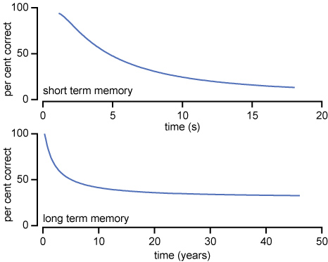
**Figure 10.** Typical retention data from idealized long- and short-term memory experiments.
Download figure:
Standard image

Using these data, we could attribute forgetting to a slow change in the synaptic strength back to its initial value with time, which may best be described as relaxation. However, this model is very simple and does not reflect the results of experiments with, e.g., rats. In these investigations, LTP was depotentiated after the rats were exposed to novel environments [54, 55]. Furthermore, Manahan–Vaughan and Braunewell showed rats a holeboard, i.e. a stimulus-rich environment, and reported [56] The observation that LTD facilitation occurred only during the initial exposure to the holeboard, whereas reexposure had no facilitatory effect on LTD, supports the intriguing possibility that exploratory learning may be associated with LTD expression. Finally, Ge et al reported that hippocampal long-term depression is required for the consolidation of spatial memory [57]. The LTP-blocking GluN2A antagonist had no effect on spatial memory consolidation, whereas two LTD-inhibiting agents disrupted the consolidation.

However, these processes are very difficult to break down to the single-neuron level. Nevertheless, Chang et al compared memristor retention loss with the memory loss of a human [58]. They demonstrated that the relaxation of the resistance value could be used to mimic short-term to long-term memory transitions in a biological system. In the following paragraphs, LTD will always be used as the analogue of LTP, with an opposite sign of the change in connection strength.

2.3. Spike timing-dependent plasticity

We have observed that the synaptic connection strength can be modified by LTP and LTD. However, we have to determine the criteria for when to apply the former or the latter to an existing neural connection. These criteria are essential characteristics of a biological neural network. In this context, Bi and Poo wrote [59]: The effects of precise timing of spikes in the presynaptic and postsynaptic neurons may be used in neural networks to decipher information encoded in spike timing [60–62] and to store information relating to the temporal order of various synaptic inputs received by a neuron during learning and memory [63, 64].

The mechanism that controls the plasticity of a connection is called spike timing-dependent plasticity or short STDP. This mechanism is a sophisticated process that can be understood as a causality detector. The basic mechanism is shown in figure 11(a). We assume that a stimulus reaches the neuron through input 1, which is connected with a synaptic strength of α. If that stimulus triggers an output spike, the output spike has a positive time delay. In other words, the output pulse occurs after the input pulse, and the positive delay times increase the synaptic connection strength. If the output pulse is caused by a stimulus of input 2 or 3, it may occur before the input 1 stimulus reaches the neuron. Then, there is no causality between input 1 and the output pulse. Consequently, the connection strength α is weakened in cases of negative delay times. However, if the time delay is very large, we do not know the causality between the previous pulses through input 1 and the outgoing pulse.

This causality detector is observed in biological neurons and is depicted in figure 11(b); negative time delays of up to −25 ms lead to LTD, positive delays of up to 25 ms give rise to LTP, and long delays cause no change in the synaptic connection strength [59].

2.4. Integrate-and-fire

The preceding paragraphs described the change in the synaptic efficacy and its dependence on several parameters. However, the biological neural network has the ability to transport information by initiating spikes, i.e. short pulses of high voltage (figure 4). This process was previously investigated by Lapicque over 100 years ago [66, 67]. This process was originally known as Lapicque's model or the voltage threshold model, and it was further refined to the model known today as integrate-and-fire [68–71]. The rather simple model captures two of the most important aspects of neuronal excitability; specifically, the neuron integrates the incoming signals and generates the spikes once a certain threshold is exceeded (figure 12).

**Figure 12.** Integrate-and-fire circuits: the perfect integrate-and-fire model consists of a capacitor, threshold detector and switch (without resistor). Once the voltage reaches a threshold, the spike is fired and the switch is closed to shunt the capacitor. In the leaky version, a resistor is added that slowly drains the capacitor with time. This corresponds to leakage current through a membrane in a living cell.
Download figure:
Standard image

This behaviour is often explained using two simple electric circuits [72]. The perfect integrate-and-fire circuit consists of a capacitor, threshold detector and switch. Once a spike is fired, the switch closes and shunts the capacitor. An additional resistor is included in the leaky integrate-and-fire circuit. The resistor slowly drains the capacitor and corresponds to leakage currents in the membrane. However, the integrate-and-fire functionality of a neural network is considerably simpler to implement than the synaptic efficacy. For example, oversampled Delta-Sigma modulators, which are 1-bit analogue- digital converters, can mimic the integrate-and-fire behaviour [73, 74]. Therefore, the following paragraphs primarily describe the use of memristive systems as synapses because the integrate-and-fire functionality can be achieved using conventional CMOS-technology.

2.5. Minimal requirements

We can summarize the primary requirements for a bio-inspired neural network as follows.

(i)
Devices that act as neurons and devices that behave like synapses are needed, and the neurons are interconnected via the synapses.
(ii)
The neurons integrate inhibitory and excitatory incoming signals and fire once a threshold is exceeded.
(iii)
The synapses exhibit LTP (cooperative, associative, and input-specific), LTD, and STDP.

3. Implementations using memristive systems

The question may be asked as to why we want to construct neuromorphic systems that emulate the presented biological mechanisms. Carver Mead pioneered a considerable amount of the research on this topic and explained the reasoning in the following way [75]: For many problems, particularly those in which the input data are ill-conditioned and the computation can be specified in a relative manner, biological solutions are many orders of magnitude more effective than those we have been able to implement using digital methods. [...] Large-scale adaptive analog systems are more robust to component degradation and failure than are more conventional systems, and they use far less power. The need for less power is particularly obvious if we compare the performance of the brain of even an invertebrate with a computer CPU and contrast the power consumption. However, there are some tasks that are difficult for a human and easy for a computer, such as multiplying two long numbers, and other problems that a human can easily solve but computers fail to solve.

In 2008, the use of memristors to mimic biological mechanisms, such as STDP, was already hypothesized [76]. Snider implemented the spike time dependence using memristive nanodevices as synapses and conventional CMOS technology as neurons. He also suggested two electronic symbols for neurons and synapses [76] that have been adapted by some groups as well as in this paper; the symbols are depicted in figure 13. Furthermore, Snider indicated that we should note that STDP alone might not be sufficient to implement stable learning; more complex synaptic dynamics and additional state variables may be required and refers to work by Carpenter et al [77] as well as Fusi and Abbott [78].

**Figure 13.** Schematic symbols for synapses and neurons as used in the following paragraphs.
Download figure:
Standard image

Although Snider suggested a new paradigm that uses large-scale adaptive analogue systems, the approach still uses a global clock signal. In 2010, Pershin and Di Ventra described a small system composed of three neurons and two synapses that is fully asynchronous [79, 80]. The memristive behaviour was emulated by a microcontroller combined with other common electronic components. They demonstrated how Ivan Pavlov's famous experiment [81] can be imitated with the basic circuit depicted in figure 14 [79].

**Figure 14.** Basic circuit consisting of three neurons and two synapses as suggested by Pershin and Di Ventra representing Pavlov's dog. The output signal (salivation) depends on the input signals (sight of food and bell sound), as well as the synaptic efficacy.
Download figure:
Standard image

Initially, the output signal (salivation) is recorded in dependence on the sight of food or a bell sound. Only the sight of food (input signal 1) leads to salivation (neuron 3 output); the bell (input signal 2) is not associated with food. There is a subsequent learning period where the input 1 and input 2 signals are applied simultaneously. Afterwards, both individual input signals induce salivation. The elegant experiment demonstrates how an important function of the brain, namely associative memory [79], can be constructed with a circuit, as shown in figure 14.

A similar simulation was conducted by Cantley et al using SPICE (UC Berkeley, CA, USA) and MATLAB (Natick, MA, USA), and they noted Also, it should be pointed out that the association as presented (in figure 4) can be unlearned. This will happen when the food is continuously presented without the bell [82].

3.1. STDP, LTP and LTD

Afifi et al revisited STDP in neuromorphic networks and proposed an asynchronous implementation [83]. This asynchronous approach may better represent biological neural networks. These researchers used specifically shaped spikes and back-propagation to adapt this approach to the CMOL platform [84]. Voltage-controlled memristive nanodevices were utilized as synapses, the memristive conductance was used as the synaptic efficacy and the CMOS-based platform used conventional integrate-and-fire neurons [85]. They could demonstrate STDP very similar to the biological neurons in figure 11 in their devices. Afifi et al concluded that the special shaped spike has a vital role in the proposed learning method, and simulation results show that even non-ideal shapes don't destroy the general trend of STDP curve for LTP and LTD. This would help us to simplify the neuron circuit design [83].

Jo et al proposed another neuromorphic system that utilizes CMOS neurons and nanoscale memristive synapses [86]. Their design uses synchronous communication and, therefore, a clock. First, we will discuss the LTP and LTD of the memristive systems. Jo et al used positive 3.2 V pulses with a length of 300 µs to induce LTP. They exposed a system to 100 subsequent pulses and measured the current through the device after every pulse at a voltage of 1 V. After 100 positive pulses, they treated the device with −2.8 V pulses of equal length, which gives rise to LTD. The current constantly decreases with every pulse, and it eventually reaches its initial value. The combination of LTP and LTD in a spike timing-dependent circuit leads to STDP very similar to the biological STDP in figure 11.

A comparable experiment was conducted by Chang et al [87]. These researchers observed LTD and LTP in their devices and simulated the behaviour with the SPICE software package. In another layered system, Choi et al experimentally verified the occurrence of LTD, LTP and STDP. These nano-crossbar designs usually consist of metal–insulator–metal (MIM) structures with rather thick (≳10 nm) oxide layers. The layer stack was Pd/WO₃/W in the former and Ti/Pt/Cu₂O/W in the latter case. However, the crossbar devices are very similar to tunnel junctions. Tunnel junctions are also MIM devices, but the insulator is thinner (∼1–2 nm) allowing the electrons to tunnel from one metal electrode to the other side.

Consequently, we observed STDP in memristive tunnel junctions [15]. LTP and LTD was present in our devices depending on the bias voltage applied to the junctions; this is shown in figure 15. Thus, we also observed STDP, as illustrated in figure 16. Again, this figure is very similar to figure 11, but the time scale is seconds rather than milliseconds. In addition to the observed STDP, we suggested another mechanism that is present in magnetic tunnel junctions for use in artificial neural networks. Magnetic tunnel junctions with very thin (0.7 nm) magnesia tunnel barriers can exhibit current-induced magnetic switching, which is sometimes called spin transfer torque switching [89–91]. The torque carried by the tunnelling electrons switches the counter electrode at high current densities (10⁵–10⁶ A cm⁻²) [91]. Sometimes, the device jumps back and forth between its magnetic configurations, i.e. parallel and anti-parallel alignment of the electrodes. This behaviour is called back-hopping [92, 93] and resembles the behaviour of a spiking neuron [88].

**Figure 15.** Long-term and short-term depression in memristive, magnetic tunnel junctions. The stimulus is delivered after 4 min. The behaviour is equivalent to the biological systems shown in figure 6 (LTP) and figure 9 (LTD) on a different timescale. Stronger or subsequent stimuli can induce up to 6% resistance change.
Download figure:
Standard image

**Figure 16.** (a) STDP in our memristive, magnetic tunnel junctions. (b) A spiking neuron emulated by back-hopping in tunnel junctions that exhibit current-induced magnetic switching. Spiking neuron inset from Gray *et al* [88], reprinted with permission from AAAS.
Download figure:
Standard image

In our earlier work [94, 95], we demonstrated that tunnel junctions are an alternative system to nanowire crossbars for observing memristive behaviour. Tunnel junctions are well understood because they have been used in Josephson junctions [96], for spin-polarized tunnelling in superconductors [97] and in magnetic tunnel junctions [98] over the past five decades. These junctions can be reproducibly prepared on the 300 mm wafer scale [99] for use as, e.g. magnetic random access memory [100]. However, crossbar and memristive tunnel junction designs may require lower device-to-device variability to be used as synaptic weights in commercial products with hundreds of thousands of synapses [101].

Nevertheless, the primary advantages of neuromorphic, analogue designs are their robustness to component degradation and moderate variability [75]. For a general introduction to the Synapse project, which aims to develop a neuromorphic computer, please see From Synapses to Circuitry: Using Memristive Memory to Explore the Electronic Brain [102]. Erokhin and Fontana discuss the use of organic memristors for biologically inspired information processing [103, 104]. Furthermore, please see the paper by Pershin and Di Ventra for another perspective on memristors and memristor-based learning [105]. For a more computer science view on learning in neural networks, Carpenter provides a good review [106], whereas Snider describes instar/outstar learning with memristive devices in particular [107], and Itoh and Chua discuss logical operations, image processing operations and complex behaviors [108].

3.2. Slime molds and mazes

We will now discuss more complex mechanisms that are not necessarily based on LTP, LTD and STDP. We will begin with a discussion on maze-solving techniques. Pershin and Di Ventra provide a nice introduction to mazes as follows [109]: Mazes are a class of graphical puzzles in which, given an entrance point, one has to find the exit via an intricate succession of paths, with the majority leading to a dead end, and only one, or a few, correctly solving the puzzle.

The maze in figure 17 can be solved by an organism as primitive as a Physarum polycephalum. To solve the maze, two food sources are placed at the entry and exit points. Then, Nakagaki et al observed that to maximize its foraging efficiency, and therefore its chances of survival, the plasmodium changes its shape in the maze to form one thick tube covering the shortest distance between the food sources. This remarkable process of cellular computation implies that cellular materials can show a primitive intelligence [111–114].

The learning behaviour of the unicellular organism Physarum polycephalum inspired the memristor-based solutions developed by Pershin et al. In 2009, they presented a model using an LC oscillator and a memristor, which are both simple, passive elements, that demonstrated pattern recognition and event prediction [115]. They reported on how the circuit can learn the period of temperature shocks. Furthermore, the circuit was able to predict when subsequent shocks were due. They identified several parameters in the amoeba that are crucial for the learning ability of the organism and established corresponding parameters in the electronic circuit. For example, the information-containing parameters correspond to the veins, and low-viscosity channels in the amoeba correspond to the resistance of the memristor in the circuit. They concluded [115] that this model may be extended to multiple learning elements and may thus find application in neural networks and guide us in understanding the origins of primitive intelligence and adaptive behaviour.

In 2011, Pershin et al returned to the original problem of solving a maze [109]. The maze can be encoded using a periodic array of memristors. The memristors are connected in an alternating head-to-head and tail-to-tail checkerboard pattern. The state of the switches between the crossing points corresponds to the topology of the maze. The maze can be solved by the simple application of a voltage across the entry and exit points. The memristors subsequently change their resistance and not only find a possible solution but also find all of the solutions in multi-path mazes and grade them according to their length. The resistance value of the memristor correlates with the length of the path, where low and high resistances indicate short and long paths, respectively. The advantage of this solution is the requirement of only one computational step; the timescale is given by the timescale of the resistance change in the memristors. Therefore, this solution is a good example of the parallel execution in this type of analogue computer; there is no internal clock. However, the read-out of the solution, as proposed by Pershin and Di Ventra, is slow; all switches are turned to the off state, and a low voltage across a single memristor determines its resistance. This process is repeated for all of the memristors, and the resistances are subsequently mapped to read out the computed solution.

3.3. Giant squid axons

In 1963, the Nobel Prize in Physiology and Medicine was awarded to Sir John Carew Eccles, Alan Lloyd Hodgkin and Andrew Fielding Huxley for their discoveries concerning the ionic mechanisms involved in excitation and inhibition in the peripheral and central portions of the nerve cell membrane [116]. Hodgkin and Huxley selected a squid for their investigations and developed an electrical circuit model of the axon membrane, which is currently referred to as the Hodgkin–Huxley equations [117]. The squid was selected because of the size of its axon, which is up to 1 mm in diameter [118]. An axon conducts the electrical impulses of a cell, e.g., towards another cell. The size of the squid's axon allows an easy installation of electrodes for measuring voltages. The squid uses this particular axon to quickly expel water initiating short, but fast movements.

The Hodgkin–Huxley electrical circuit is shown in figure 18, where three different currents are displayed: the sodium ion current (I_Na), the potassium ion current (I_K), the leakage current (I_l), adding up to the axon membrane current (I) [117]. The same process can be performed for the corresponding voltages and resistances. Hodgkin and Huxley described the large axon as chains of Hodgkin–Huxley-cells, which are paired by diffusive/dissipative couplings. In certain approximations, this pairing can be described based on standard diffusion mechanisms [119]. The values of the circuit elements, e.g. the voltages, have to be determined experimentally. The resistances R_K and R_Na are time-varying resistances. In this context, Chua wrote [120] However, the terms 'time-varying resistance' and 'time-varying conductance' chosen by Hodgkin and Huxley are unconventional in the sense that R_K and R_Na in the HH Circuit model cannot be prescribed as a function of time, as is generally assumed to be the case in basic circuit theory [121, 122]. There are also additional inconsistencies with the original circuit chosen by Hodgkin and Huxley. Mauro pointed out the following [123]. It was discussed by Cole [124] in 1941 in connection with the interesting discovery in 1940 by Cole and Baker [125] that under certain conditions the squid axon displayed positive reactance in AC bridge measurements. However, in 1972, Cole himself wrote [126] The suggestion of an inductive reactance anywhere in the system was shocking to the point of being unbelievable.

Recently, Chua took all of these points into consideration and suggested a new electrical circuit to replace the original circuit developed by Hudgkin and Huxley [4, 120, 127], this circuit is shown in figure 19. The two time-variable resistors are replaced by a first-order memristor for the potassium channel and a second-order memristor for the sodium channel. This result reconciles all of the anomalous behaviours in the Hodgkin–Huxley model, such as the absence of rectifiers and large inductances in the brain and the lack of matching magnetic fields.

**Figure 19.** Alternative electrical circuit model for the giant squid axon as suggested by Chua. The time-variable resistors are replaced by first- and second-order memristors for the potassium and sodium channels, respectively.
Download figure:
Standard image

4. Conclusions

In this paper, we aimed not only to review some of the research in the field of memristor-based neural networks but also to demonstrate the excitement and fast pace that have motivated this field in the past few years. The human brain and associated mechanisms, such as learning and forgetting, are naturally fascinating, and neuromorphic computers that mimic these mechanisms are interesting for technological applications and fundamental science. Although conventional CMOS technology is capable of emulating the integrate-and-fire operation of a neuron, the functionality of a synapse is more difficult to mimic in a simple electrical circuit. However, a basic, passive, two-terminal device called a memristor can easily realise synaptic behaviour. On the one hand, this process enables the development of adaptive, analogue computer systems, which are more robust and consume less power than their conventional counterparts. On the other hand, this approach permits the use of basic electrical circuits as a model for biological systems, such as the presented Hodgkin–Huxley model.

Acknowledgments

The authors would like to thank Barbara and Christian Kaltschmidt for many helpful discussions about memristors and its relation to biological systems. They are grateful to Günter Reiss and Andreas Hütten for their continuous support of their work. Also, they would like to thank Patryk Krzysteczko, Jana Münchenberger, Stefan Niehörster, Marius Schirmer and Olga Simon. This work was funded by the Ministry of Innovation, Science and Research (MIWF) of North Rhine-Westphalia with an independent researcher grant.

Memristor-based neural networks

Article metrics

Submit

Permissions

Author e-mails

Author affiliations

Dates

Abstract

1. Introduction