


Abstract
We present the four-year survey results of monthly submillimeter monitoring of eight nearby (<500 pc) star-forming regions by the JCMT Transient Survey. We apply the Lomb–Scargle Periodogram technique to search for and characterize variability on 295 submillimeter peaks brighter than 0.14 Jy beam−1, including 22 disk sources (Class II), 83 protostars (Class 0/I), and 190 starless sources. We uncover 18 secular variables, all of them protostars. No single-epoch burst or drop events and no inherently stochastic sources are observed. We classify the secular variables by their timescales into three groups: Periodic, Curved, and Linear. For the Curved and Periodic cases, the detectable fractional amplitude, with respect to mean peak brightness, is ∼4% for sources brighter than ∼0.5 Jy beam−1. Limiting our sample to only these bright sources, the observed variable fraction is 37% (16 out of 43). Considering source evolution, we find a similar fraction of bright variables for both Class 0 and Class I. Using an empirically motivated conversion from submillimeter variability to variation in mass accretion rate, six sources (7% of our full sample) are predicted to have years-long accretion events during which the excess mass accreted reaches more than 40% above the total quiescently accreted mass: two previously known eruptive Class I sources, V1647 Ori and EC 53 (V371 Ser), and four Class 0 sources, HOPS 356, HOPS 373, HOPS 383, and West 40. Considering the full protostellar ensemble, the importance of episodic accretion on few years timescale is negligible—only a few percent of the assembled mass. However, given that this accretion is dominated by events on the order of the observing time window, it remains uncertain as to whether the importance of episodic events will continue to rise with decades-long monitoring.
Export citation and abstract BibTeX RIS
1. Introduction
Mass accretion is the key process of star formation; however, the time dependence is not yet well-understood (see review by Dunham et al. 2014). The Luminosity Problem, a potential discrepancy between observed luminosities of YSOs and the luminosities expected from theory, was uncovered by Kenyon et al. (1990), and updated by Evans et al. (2009) and Dunham et al. (2010), following observations by the Spitzer Space Telescope. The episodic accretion model for protostellar assembly, which has quiescent-accretion phases interspersed with burst-accretion phases, has been suggested as a possible solution to this discrepancy. Other solutions require that most of the accretion occurs very early in the protostellar evolution (e.g., Offner & McKee 2011; Fischer et al. 2019)
Some support for the episodic accretion hypothesis can be found among young eruptive variable stars, which show a significant increase in their optical and near-IR brightness due to abrupt changes in the accretion rate (Hartmann & Kenyon 1996). Based on photometric (Hartmann et al. 1998; Scholz et al. 2013; Hillenbrand & Findeisen 2015; Contreras Peña et al. 2017, 2019; Fischer et al. 2019), chemical (Jørgensen et al. 2015; Hsieh et al. 2019), and outflow (Bontemps et al. 1996) surveys, outburst events appear to occur more frequently during the earliest evolutionary stage of formation, in agreement with theoretical (Machida et al. 2011; Bae et al. 2014; Vorobyov & Basu 2015) studies. Furthermore, during this early stage, while the protostar remains deeply embedded in its natal envelope, most of the stellar mass is gained. Therefore, carefully studying the variability of protostars that are densely enshrouded is essential to understanding the effects of mass accretion variability during the star formation process.
Searches for variability of YSOs using optical and infrared data have been effective for discovering variable accretion in the later stages of star formation. Deeply embedded protostars (Class 0), however, are difficult to detect at optical and near-IR because of their thick envelope, which absorbs the short-wavelength radiation from the central protostar and re-emits it thermally, at much longer wavelengths. Johnstone et al. (2013) modeled the effect of enhanced accretion on dust emission from the heated envelope and found that the thermal response timescale to accretion luminosity changes at the protostar should be weeks to months, limited only by the envelope light-crossing time, as the dust is quick to thermally equilibrate.
The possibility of detecting submillimeter variability on months-long timescales motivated the JCMT Transient Survey (Herczeg et al. 2017). We are monitoring eight nearby star-forming regions at 450 and 850 μm at an approximately monthly cadence using the Submillimetre Common-User Bolometer Array 2 (SCUBA-2; Holland et al. 2013) on the James Clerk Maxwell Telescope (JCMT). Roughly 100 protostars in these fields are bright enough for evaluating variability, with a relative flux accuracy of ∼2% achieved by careful calibration (Mairs et al. 2017a).
In our previous paper, Johnstone et al. (2018) investigated the stochastic and linear secular variability of 150 submillimeter emission peaks, both protostellar and pre-stellar, over the first 18 months of the monitoring survey. In that paper, we uncovered six robust protostellar variables by fitting linear trends to the submillimeter light curves and measuring the observed epoch to epoch submillimeter brightness standard deviations. Five out of 50 protostars were found to be secularly (linearly) variable. One source, EC 53 (V371 Ser) in the Serpens Main region (see also Yoo et al. 2017; Mairs et al. 2017b), was found to have a significant stochasticity. EC 53 had previously been observed to vary periodically in the near-IR (Hodapp et al. 2012), with a timescale of 1.5 yr. More detailed analysis of EC 53 (Lee et al. 2020b) reveals a similar periodic variability in submillimeter brightness as well as for the near-IR color, the latter produced by the combination of variable brightness and extinction associated with the underlying accretion process (Lee et al. 2020b). The secular variability found in EC 53 allows for a quantitative determination of accretion-related amplitudes and timescales and a qualitative discussion of the physical instabilities driving the observed periodicity. These results also motivate a detailed search for similar periodic trends in the submillimeter light curves toward our full sample of embedded protostars.
In this paper, we examine protostellar variability beyond the linear trend by applying the Lomb–Scargle Periodogram (LSP; Lomb 1976; Scargle 1989; VanderPlas 2018) analysis to the first four years of monitoring measurements obtained by the JCMT Transient Survey. In Section 2, we summarize the JCMT Transient Survey observing methods and describe the data reduction process, including precision relative pointing and flux calibration. In Section 3, we present the analysis methods that are applied to find protostellar variability from the submillimeter light curves. We separate the secular variability, extracted from our LSP and linear analysis (Section 3.1), and the stochastic variability, found after subtracting any secular variability (Section 3.2). In Section 4, we determine the completeness of our secular variability analysis as a function of source brightness. In Section 5, we discuss the ensemble variability statistics with respect to individual regions and to protostellar evolutionary stage (Sections 5.1 and 5.2), and compare the submillimeter light-curve behavior of sources identified at shorter wavelengths as either bursting (Section 5.3) or appearing subluminous (Section 5.4). In Section 6, we summarize our results.
2. The JCMT Transient Survey
The JCMT Transient Survey (Herczeg et al. 2017) uses the Submillimetre Common User Bolometer Array 2 (SCUBA-2; Holland et al. 2013) to observe continuum emission simultaneously at 450 and 850 μm with effective beam sizes of 9.8'' and 14.6'', respectively (Dempsey et al. 2013). Since 2015 December, the survey has monitored eight star-forming regions within 500 pc of the Sun: IC 348, NGC 1333, NGC 2024, NGC 2068, Orion Molecular Cloud (OMC) 2/3, Ophiuchus, Serpens Main, and Serpens South. All but Serpens Main are monitored at an approximately monthly cadence as weather conditions and target observability allow, while Serpens Main is monitored twice per month to provide additional information on the accretion variability of deeply embedded protostar EC 53 (Yoo et al. 2017; Lee et al. 2020b). In this paper, we include almost all monitoring data obtained from the beginning of the survey through 2020 January. Three observations of NGC 1333 on 2016 February 5, 2017 December 8, and 2018 July 07, as well as one observation of OMC 2/3 observed on 2018 March 8 (less than 2% of our observations) are excluded due to anomalously high uncertainty in the relative spatial alignment of the final maps (see Table 1).
Table 1. Observation Summary by Region
| Region | Start Date | Last Date | # of Epochs | Nsubmm a | Ndisk | Nprotostar |
|---|---|---|---|---|---|---|
| IC 348 | 2015 Dec 22 | 2020 Jan 24 | 35 | 9 | 0 | 5 |
| NGC 1333 | 2015 Dec 22 | 2020 Jan 24 | 34 b | 31 | 1 | 16 |
| NGC 2024 | 2015 Dec 26 | 2020 Jan 24 | 35 | 36 | 3 | 3 |
| NGC 2068 | 2015 Dec 26 | 2020 Jan 24 | 36 | 29 | 0 | 15 |
| OMC 2/3 | 2015 Dec 26 | 2020 Jan 24 | 33 b | 95 | 13 | 14 |
| Ophiuchus | 2016 Jan 15 | 2020 Jan 18 | 28 | 33 | 5 | 9 |
| Serpens Main | 2016 Feb 02 | 2019 Oct 19 | 50 | 16 | 0 | 8 |
| Serpens South | 2016 Feb 02 | 2019 Nov 02 | 35 | 46 | 0 | 13 |
Notes.
a Total number of detected submillimeter sources (>0.14 Jy beam−1), including disks, protostars, and prestellar cores. b Three epochs of NGC 1333 and one epoch of OMC 2/3 have been excluded from the analysis because of poor telescope pointing.Download table as: ASCIITypeset image
The observations employ the Pong1800 (Kackley et al. 2010) scan pattern to produce a circular field  in diameter with uniform background rms noise. During each observation, the telescope scans across the sky at a rate of 400'' s−1 such that each part of the target field is observed from multiple position angles. This strategy allows for the separation of telluric contributions and astronomical source contributions to the flux in the data reduction process. The observations are performed up to a maximum zenith opacity at 225 GHz (τ225) of 0.12, corresponding to precipitable water vapor of <2.58 mm, as measured by the JCMT line-of-sight 183 GHz water vapor radiometer (Dempsey et al. 2013). Depending upon the sky conditions, the integration time is between 20–40 minutes, in order to yield a consistent sensitivity of ∼14 mJy beam−1 at 850 μm (Mairs et al. 2017a). The atmospheric transmission in the 450 μm band, however, has a much stronger dependence on precipitable water vapor, yielding more than an order-of-magnitude variation in rms noise, and thus analysis of the 450 μm survey data are deferred to a future publication.
The data are reduced using the iterative makemap (Chapin et al. 2013) software, found in starlinks (Currie et al. 2014) Submillimetre User Reduction Facility (smurf) package (Jenness et al. 2013). No 12CO subtraction was performed at 850 μm. The standard JCMT observing scheme and data reduction pipeline yields a pointing uncertainty of ∼2 or 3'' and a flux calibration uncertainty of ∼5%–10% (Dempsey et al. 2013). All observations presented in this work are then post-processed to improve spatial alignment and reduce the flux calibration uncertainty in a relative sense (epoch to epoch). Using the methods described in Mairs et al. (2017a), the locations of bright, compact point sources are measured from epoch to epoch to derive pointing corrections in order to align the images to better than 1''. In addition, by monitoring the peak fluxes of a set of bright, non-varying sources over time, relative flux calibration factors are derived for each epoch, reducing the flux calibration uncertainty at 850 μm to 2%. 35
We investigate all eight Transient Survey fields, limiting our analysis to those sources within 18' of each mapping center where the map noise properties are uniform. Among 1665 submillimeter peaks identified through clump-finding (Johnstone et al. 2018) with the FellWalker algorithm (Berry 2015), we analyze 295 sources with the mean peak brightness greater than 0.14 Jy beam−1, corresponding to a signal-to-noise per epoch of ∼10.
Our final sample contains submillimeter peaks coincident to within 10 arcseconds of 22 disk (Class II) objects and 83 protostars (Class 0/I), which have previously been classified through their SEDs (Dunham et al. 2010; Stutz et al. 2013; Megeath et al. 2016). Table 1 provides the numbers of submillimeter sources, protostars, and disks per star-forming region, along with the number and date range of the epochs observed.
3. Analysis
Following the methodology by Johnstone et al. (2018), we separate our variability analysis into two investigations dependent on the light-curve properties. We refer to those sources with light curves that can be modeled as smoothly varying over the 4.5 years of monitoring as "secular," and those with light curves more likely due to either singular or ongoing discrete events are termed "stochastic." We note that the labels secular and stochastic implicitly depend on a timescale and are sometimes defined differently. For example, Dunham et al. (2014) used the term stochastic to refer to any variability arising from random processes over a wide variety of timescales, while using the term secular to refer to very slow, long-term changes in accretion rates that occur over the full lifetime of the embedded phase. When contemplated over such longer times, the secular variations uncovered here may be interpreted as stochastic, with time constants of at least several years.
3.1. Secular Variability
We first examine secular variability, i.e., changes that take place across the entire time coverage. We determine the amplitudes and timescales associated with the observed brightness fluctuations, and then use these measurements to classify the types of variability. Furthermore, these estimates for the timescales involved in the observed variations provide a direct link to the underlying physical process responsible for the variations (e.g., viscously evolving disks, Keplerian orbit times).
We apply an LSP (Lomb 1976; Scargle 1989; VanderPlas 2018) analysis in order to uncover and quantify the relevant timescales and amplitudes of secular variability observed in the submillimeter. The LSP measures the likelihood that an observed light curve is fit well by a sinusoidal function with a set of parameters: mean brightness, amplitude, frequency, and phase. The statistical power measures the quality of the best sinusoidal fit as a function of frequency and builds the periodogram of the observed light curve. We perform the LSP analysis using the LombScargle task in the timeseries package of astropy (Astropy Collaboration et al. 2013) and analytically modify the output to fit our purpose. The details of the LSP output and our modifications are described below.
In the LSP analysis, the statistical power PA of the "A" hypothesis is defined as the fractional improvement over the non-varying (or static) "N" hypothesis:
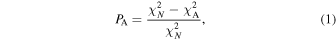
where  denotes the chi-squared value of the subscripted hypothesis. Thus, the value of PA
rises as the goodness of fit of the sinusoidal function improves on the non-varying hypothesis; that is,
denotes the chi-squared value of the subscripted hypothesis. Thus, the value of PA
rises as the goodness of fit of the sinusoidal function improves on the non-varying hypothesis; that is,  reduces with respect to
  . Following standard practice, we consider the frequency at which PA reaches its maximum value to denote the best fit.
We next determine the False Alarm Probability (FAP) of this best fit to validate the detection. The FAP measures the probability that the sinusoidal fit is not real. The FAP is calculated using the best-fit χ2 (Baluev 2008). That is, the FAP of the best-fit "A" hypothesis, FAPA, is defined as

The FAP decreases with increasing degrees of freedom in the fit Nf = (Nepoch − DA), where Nf is determined from the number of epochs observed, Nepoch, minus the number of parameters in the model, DA. The FAPA also reduces as the fractional improvement of the sinusoidal fit PA increases.
Following the traditional LSP approach, the FAP of the best hypothesis must also take into account the total number of hypotheses tested. Thus, we define FAPLSP as

where Nfreq is the total number of frequencies tested. Furthermore, since we are only interested in cases where FAPA ≪ 1, this can be significantly simplified to

Most protostellar sources are best fit by low-frequency, long-timescale, sinusoids. Very short-period sinusoids always result in poor fits to these protostellar light curves. The tested frequency range and step is calculated using the time baseline and the number of observed epochs. Using our 4 yr time baseline and 35 epochs, the tested frequencies are between 0.025 yr−1 (once in 40 yr) and 22 yr−1 (almost once per two weeks) with 0.05 yr−1 steps. The traditional FAPLSP calculated over the full tested frequency range, which includes very high frequencies, will provide a systematic overestimate of the false alarm probability. We therefore modify the FAPLSP to consider only periods longer than the best-fit period, with  given by

where N<freq is the number of tested periods that are longer than or equal to the best-fit period (lower than the best-fit frequency). Thus,  becomes equivalent to FAPLSP for sources with best-fit periods similar to the highest frequency tested.
Given that our LSP analysis uncovers primarily long-period sinusoids, often with periods greater than the 4 yr observing window, we also apply a linear least-squares fitting method to quantify the best-fit linear solution. The statistical power, PLin, and the FAP of the linear best fit, FAPLin, are calculated following Equations (1) and (2).
We demonstrate our dual secular analysis procedure in Figure 1, where the bottom panel plots the 4 yr light curve for a known variable (EC 53 in Serpens Main; see also Lee et al. 2020b). We first perform the LSP analysis and reproduce the periodogram in the upper left panel. We next diagnose the various FAPs derived at the peak of the periodogram, denoted by the vertical orange line. For this source, the periodogram peak is found at a frequency of 0.0017 day−1, equivalent to a 1.61 yr period, the single-frequency false alarm probability is less than 10−11, and both the LSP and modified FAPs are less than 10−8, denoting that the sinusoidal fitting is highly faithful. Finally, we also determine the best-fit linear form (dashed orange line in upper panel) and calculate a large linear FAP, greater than 0.5, denoting the linear fit has a 50% likelihood of being a false alarm.
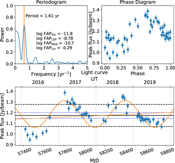
Figure 1. Periodogram, phase diagram, and light curve for known variable source EC 53 in Serpens Main (see also Lee et al. 2020b). Upper left panel: Periodogram for EC 53. The solid orange vertical line indicates the frequency of the peak statistical power. The FAPs shown in the panel are calculated following Equations (2)–(5). Upper right panel: Phase diagram for EC 53. The period of 1.61 yr found by the periodogram analysis is used for folding the light curve. Lower panel: light curve for EC 53. The black solid line indicates the mean peak brightness over the full time window, in Jy beam−1. The black dashed lines and blue dotted lines indicate the observed standard deviation and fiducial uncertainty around the mean peak brightness, respectively. The solid orange curve denotes the best fit sinusoid recovered from the LSP analysis. The dashed orange straight line denotes the best-fit linear function. MJD is JD–2400000.5.
Download figure:
Standard image High-resolution imageIn Figure 2, we show examples of sources with light curves fit robustly by either periodic or linear secular functions. The top panel shows a periodic light curve with short period compared to our time coverage (4 yr). The second panel from the top shows a light curve robustly fit by a sinusoid with a period comparable to 4 yr, but not by a linear function. The bottom two panels show light curves fit well by both sinusoidal and linear functions, where the sinusoidal period is much longer than the time baseline. We specify the classification of the found variables and analyze their properties in Section 3.3.
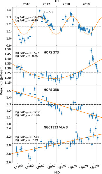
Figure 2. Representative light curves found in this study. The top two panels show Periodic and Curved light curves, while the lower two panels are increasing and decreasing Linear light curves. In all cases, the black horizontal line indicates the mean peak flux of the source over all epochs. The orange solid line shows the sinusoidal best fit of the light curve, and in the bottom two panels the orange dashed line shows the linear best fit.
Download figure:
Standard image High-resolution imageTo confirm the robustness of our method, in Figure 3 we compare the FAPs of the two fitting functions, sinusoidal and linear, for each of the 295 submillimeter sources in our sample. In the figure, we color-code the sources by type: protostar (red), disk (blue), and starless (gray). The starless cores and disk sources occupy the lower left corner of the plot, where there is no robust evidence for secular variability (i.e., FAPs > 0.1%).
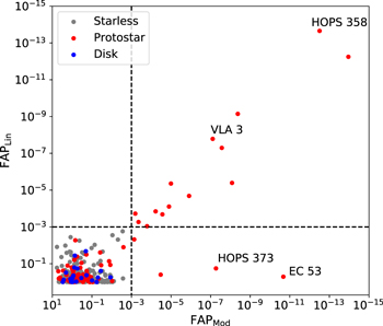
Figure 3. Comparison of the sinusoidal,  , and linear, FAPLin, false alarm probabilities for all 295 submillimeter sources in our sample. The black dashed lines correspond to FAPs of 0.1% along each axis. Sources are color-coded by type as shown in the inset legend.
Download figure:
Standard image High-resolution imageEighteen protostellar sources are found significantly outside the lower left corner of Figure 3. Furthermore, all 14 protostellar sources that have FAPLin < 0.001 also have  and lie along a diagonal line in the figure. This is expected, given that long-period sinusoids are almost indistinguishable from linear functions over limited timescales. In the figure, however, there are an additional four protostellar sources with
  for which a linear fit is poor due to the observed periodicity or curvature of the light curve. While EC 53 (see Figure 1) shows clear periodic variability, the other three sources, HOPS 315, HOPS 373, and SMM 10, reveal clear curved trends with little overall slope and have best-fit periods of < 8 yr; see the light curves of HOPS 315 (Figure B1.9), HOPS 373 (Figure 2), and SMM 10 (Figure B1.5). We discuss further all of the revealed secular variables in Section 3.3.
It is important to note that the LSP determination of a robust sinusoid fit does not necessarily imply that the underlying source variability is truly periodic, especially for the majority of our uncovered sources (16 out of 18) requiring long periods, on the order of or greater than the 4 yr observing time window. Nevertheless, the best-fit parameters provide a useful, quantifiable estimate of the underlying timescale and amplitude for observed light-curve variations. We stress, however, that for periods longer than 4 years, these are extrapolated estimates of the period and amplitude of the observed light-curve event and not an indication of underlying periodicity. Additionally, for the longest robust sinusoidal fits, the periods of the amplitudes are extremely uncertain and the linear slopes are more appropriate quantifiable measures of the variability. Thus, in general we will use sinusoidal fits only for sources with derived periods less than ∼15 years.
3.2. Stochastic Variability
Along with the long-term secular variability, sources may vary irregularly, with timescales of a few months or shorter. Two types of stochasticity are anticipated: (1) long-term chaotic brightness variations resulting in an increase in the epoch-to-epoch brightness variability without an appreciable linear or periodic trend, perhaps due to short-timescale instabilities near the disk/star interface; (2) rare, individual epoch brightening or dimming events that robustly stand out above the noise. We explore both of these stochastic variability possibilities across all observed epochs for each of the 295 submillimeter sources in our sample.
We first consider the rare, individual epoch events. The expected uncertainty of each peak brightness measurement of a given submillimeter source at 850 μm is defined as the fiducial uncertainty, σfid, and calculated as

where  is the mean peak brightness of the source over all observations. The other two terms in Equation (6) are the relative flux calibration error for a given map epoch, 2%, and the typical 850 μm rms noise, 0.014 Jy beam−1. These values have been empirically measured for the JCMT Transient Survey by Mairs et al. (2017a), and the fiducial uncertainty is described in detail by Johnstone et al. (2018). To mitigate the effect of outlier measurements on the mean peak brightness, we determine the mean peak brightness after excluding the brightest and faintest 10% of measurements from each source,
  , and we use this value in place of
  in Equation (6). Furthermore, for the 18 secular variables uncovered in Section 3.1, we subtract the best-fit sinusoidal function from their light curves before determining
  .
.
We first analyze the light curves of all 295 submillimeter sources in our sample for individual outlier events. For each measurement of each source, including the brightest and faintest 10%, we determine the residual peak brightness after subtracting  . We then bring these residual measurements to a standard scale by dividing by the expected measurement uncertainty σfid. Figure 4 presents a histogram over all these σfid scaled residual fluxes (light), and after excluding the 18 secular variables (dark).
Figure 4. Histogram of the stochasticity,  , of each measurement of all 295 submillimeter sources in our sample (light), and after excluding the 18 secular variables (dark). Where necessary, the stochasticity is obtained after subtracting the best-fit sinusoidal function. The black dashed line overlays the Gaussian function obtained by the standard deviation (σ = 1.10) and mean (0.01) of the stochasticity. The red lines show where the stochasticity equals to±5. The red histogram denotes the outlier detected in HOPS 373.
Download figure:
Standard image High-resolution imageThe shape of the distribution follows well the expected normal distribution with an standard deviation fit close to unity, σ = 1.10, indicating that our uncertainty estimates are appropriate. The residuals with absolute values greater than 3, however, are somewhat overpopulated, perhaps indicating slight non-Gaussian shape in the noise characteristics. In addition, there are six highly stochastic events with absolute residuals greater than 5, indicated by the red vertical lines in the figure. These six candidate stochastic events (Table 2) are measured across six different sources, five of which are known protostars,
Table 2. Candidate Stochastic Events
| Region | ID | Known Name |
 ( ( )
a )
a
|

| Fmax/
| Date | Robust? |
|---|---|---|---|---|---|---|---|
| (Jy beam−1) | (σfid) | (light curve) | |||||
| NGC 2068 | J054631.0−000232 | HOPS 373 | 1.25 (1.26) | 5.34 b | 1.12 | 2019 Sep 26 | Yes (Figure 2) |
| OMC2/3 | J053522.4−050111 | HOPS 88 | 2.50 (2.50) | 6.80 | 1.14 | 2016 Feb 29 | No/Focus |
| Serpens south | J183002.6−020248 | CARMA 3 | 2.19 (2.20) | 6.43 | 1.13 | 2019 Nov 2 | No/Focus |
| OMC2/3 | J053527.4050929− | HOPS 370 | 2.62 (2.64) | 5.79 | 1.11 | 2017 Apr 21 | No/Focus |
| NGC 2068 | J054645.6 + 000719 | LBS 11 | 0.32 (0.32) | 5.48 | 1.26 | 2016 Apr 27 | No/Extended |
| OMC2/3 | J053524.2−050932c | starless | 0.34 (0.34) | −5.01 | 2018 Nov 2 | No/Extended |
Notes.
a The values in the bracket denote the mean peak brightness using the whole data points (see Section 3.2.) b Value obtained after subtracting the best-fit sinusoidal function.Download table as: ASCIITypeset image
Two of the six candidate stochastic events are associated with faint submillimeter sources,  Jy beam−1, for which the fiducial uncertainty is dominated by measurement error (Equation (6)). This sample includes the only non-protostellar potential variable source in our sample, and also the only source to apparently dim for a single epoch. Careful examination of the residual images, after subtracting the co-add over all epochs from the epoch in which the event occurred, reveals that for both these candidates the residual emission is extended significantly beyond that of a point source. These results strongly suggest that for these two epochs the image reconstruction procedure has introduced spurious large-scale features, not unexpected in submillimeter map reconstructions (for details, see Mairs et al. 2015, 2017a). We therefore drop these two candidates as potential stochastic events.
Three of our candidate stochastic events are bright,  Jy beam−1, but reside nearby, r < 30'', vastly brighter sources,
  Jy beam−1. For each of these candidates, the residual images for the epochs of interest show clear structure in the residual beam pattern of all the brighter sources within the map, indicating slight focus issues during the observation. The focus issue is seen to clearly produce excess emission within r ∼ 30'' around the brighter sources, and thus the measurement uncertainties for the three candidate stochastic events are significantly underestimated at these particular epochs. We therefore drop these three candidates as potential stochastic events.
Finally, one of our protostellar sources, HOPS 373 (see Figure 2 and Table 2), is detected in both the secular and stochastic variability analyses. We therefore note that the stochastic event detected in HOPS 373 appears to be part of a longer-timescale burst-like event. Comparison of the residual map for the epoch in which the >5σ stochastic event occurred reveals a strong point-like significant peak at the location of HOPS 373, assuring the robustness of the detection. Given that this brightening event occurs over more than one epoch, 36 we categorize this source as a secular variable in the rest of this work.
Mairs et al. (2019) performed a separate single-epoch transient source analysis for those areas within our monitored star-forming regions where there are no bright submillimeter sources. That investigation uncovered a prominent stochastic submillimeter variable, coincident with JW 566 in OMC2/3. JW 566 is a T Tauri star and shows a brightening by 500 mJy in a single epoch and a ∼50% decline in its peak brightness during the half-hour observation. The mean brightness of JW 566 over all epochs lies below the threshold used for this paper, however, and therefore JW 566 is not identified by, or included in, our analysis.
Having found no robust rare, individual epoch events within our sample of bright sources, we next consider the measured peak brightness uncertainty over the full light curve, normalized by the expected fiducial uncertainty, as a determination of the long-term stochastic nature of each of our 295 submillimeter sources. Here, we are searching for sources with a significantly larger spread in brightness measurements compared with the known noise properties of the measurements. Figure 5 plots this dispersion against mean peak brightness, with color again indicating source type. The y-axis plots  , the chi-square obtained by using only the flux measurements that went into calculating
  . Thus, any rare significant outlier events are not included in this analysis. The eighteen known secular variables are marked with black circles, and HOPS 373 with the individual stochastic event is marked with cross. The left panel presents the calculation before removing the best-fit sinusoid from the secular variables, whereas the right panel shows the result after subtracting the secular trend.
Figure 5. The distribution of  divided by the number of epochs (N80%) with respect to the mean peak brightness. Here, we used only the middle 80% data points, excluding each 10% of the brightest and faintest fluxes from the light curves. Circles denote sources with robust secular variability. The cross denotes the source (HOPS 373) with individual epoch stochastic variability. Right panel is the same as the left panel, except that the
  is calculated after subtracting secular trends from the light curves of robust secular variables. The black and red dashed lines indicate
  and 1.8, which correspond to χ2/N = 1 and 4, respectively, assuming a Gaussian distribution.
Download figure:
Standard image High-resolution imageTwo results are immediately evident in Figure 5. First, all sources in the left panel with anomalously large variations in the measured peak brightness over their full light curves,  (corresponding to an expected χ2/N ∼ 4 when measured over a full Gaussian distribution), are secular variables for which the large deviations are significantly removed by subtracting the secular fit (right panel). Thus, given the present survey sensitivity, there are no sources with ongoing random brightness variations significantly larger than the measurement uncertainty. Second, the typical peak brightness of the robustly determined variables is shifted to the right (brighter), compared with the full sample even when only considering protostars (red dots). This is an expected occurrence due to the increased signal-to-noise ratio for bright sources and its carryover effect on the completeness of our analyses. We return to this discussion in Section 4.
3.3. Properties of the Variables
In this section, we consider the quantifiable properties of the robustly recovered variables in our sample in order to determine an approximate classification scheme. Using a false alarm threshold criterion of 0.1% and a stochastic threshold of ± 5σ, we recover only 18 secular variables among the 295 bright submillimeter sources in our sample.
All the robust variables within our survey are known protostars. None of the known disk sources show any variability in the submillimeter using our LSP, linear, and stochasticity analyses. This absence is at least in part due to the low peak brightness of the disk sources in submillimeter (see Figure 7), and the brightness-dependent completeness discussed in Section 4. We further discuss the variability depending on evolutionary stage in Section 5.2. Limiting our sample only to protostars, we find that ∼22% (18 out of 83) are observed to be secular variables and none show evidence of a single stochastic outlier event.
Tables 3 and 4 present the quantitative results for individual secular variables. The observed amplitude (ΔF) is defined as Fmax–Fmin where Fmax and Fmin are the brightest and faintest peak brightness among the measured fluxes of a source. The LSP-derived periods of the detected variables vary from 1 year to 40 years. We categorize the variables with their best-fit periods compared to the 4 yr observing window of our survey: Periodic (<4 yr: Group P), Curved (4–15 yr: Group C), and Linear (>15 yr: Group L).
Table 3. Physical Properties of Robust Secular Variables
| Region | ID | Figure a | Known Name |

| ΔF/σfid | ΔF/
| Lbol | Tbol |
|---|---|---|---|---|---|---|---|---|
| (Jy bm−1) | (%) | (L⊙) | (K) | |||||
| IC 348 | J034356.5 + 320050 | B.1 | IC348 MMS 1 | 1.39 | 4.57 | 10.2 | 1.6 | 23 b |
| Serpens main | J182951.2 + 011638 | B.2 | EC 53 | 1.17 | 16.2 | 37.7 | 5.9 | 161 b |
| NGC 2068 | J054647.4 + 000028 | B.3 | HOPS 389 | 0.99 | 5.09 | 12.4 | 6.0 | 43 c |
| NGC 1333 | J032910.4 + 311331 | B.4 | IRAS 4A | 9.16 | 7.84 | 15.7 | 8.3 | 31 b |
| Serpens main | J182952.0 + 011550 | B.5 | Serpens SMM 10 | 0.84 | 6.21 | 16.1 | 8.3 | 70 b |
| Ophiuchus | J162626.8-242431 | B.6 | VLA 1623-243 | 3.89 | 5.42 | 11.0 | 0.5 | 45 d |
| NGC 2068 | J054613.2-000602 | B.7 | V1647 Ori | 0.25 | 7.93 | 47.3 | 27 | 322 c |
| IC 348 | J034357.0 + 320305 | B.8 | HH 211 | 1.21 | 6.59 | 15.2 | 1.4 | 23 b |
| NGC 2068 | J054603.6-001447 | B.9 | HOPS 315 | 0.52 | 3.06 | 10.2 | 6.2 | 180 c |
| NGC 2068 | J054631.0-000232 | B.10 | HOPS 373 | 1.26 | 10.9 | 25.0 | 5.3 | 37 c |
| OMC2/3 | J053529.8-045944 | B.11 | HOPS 383 | 0.54 | 5.56 | 18.1 | 7.8 | 46 c |
| NGC 1333 | J032903.8 + 311449 | B.12 | West 40 | 0.48 | 7.86 | 27.8 | 0.7 | 18 b |
| Serpens south | J182937.8-015103 | B.13 | IRAS 18270-0153 | 0.63 | 5.79 | 17.2 | 6.9 | 57 b |
| Serpens main | J182949.8 + 011520 | B.14 | Serpens SMM 1 | 7.08 | 9.35 | 18.8 | 70 | 13 b |
| Serpens main | J182948.2 + 011644 | B.15 | SH 2-68 N | 2.10 | 3.20 | 6.76 | 14 | 31 b |
| Serpens south | J183004.0-020306 | B.16 | CARMA 7 | 4.85 | 5.31 | 10.7 | 15 | 35 e |
| NGC 2068 | J054607.2-001332 | B.17 | HOPS 358 | 1.29 | 16.2 | 37 | 25 | 42 c |
| NGC 1333 | J032903.4 + 311558 | B.18 | NGC1333 VLA 3 | 3.04 | 11.3 | 23 | 38 | 220 b |
Notes.
a The reference number of the light curve in Figure Set B (online-only material). b For these sources, the Lbol and Tbol values are taken from Mowat (2018). See also Section 5.1 for more details. c For these sources, the Lbol and Tbol values are taken from Furlan et al. (2016). d For this source, the Lbol and Tbol values are taken from Murillo et al. (2018). e For this source, the Lbol and Tbol values are taken from Maury et al. (2011).Download table as: ASCIITypeset image
Table 4. Light-curve Properties of Robust Secular Variables
| Known Name | Period a | A/σfid | A/
| Slope/
| Grp b | log FAPMod | log FAPLin |
|---|---|---|---|---|---|---|---|
| (yr) | (%) | (% yr−1) | |||||
| MMS 1 | 1.05 | 1.78 | 2.70 | −1.3 | P | −3.36 | −3.27 |
| EC 53 | 1.61 | 8.77 | 10.8 | P | −10.7 | −0.29 | |
| HOPS 389 | 4.53 | 2.69 | 3.17 | −1.5 | C | −4.90 | −5.39 |
| IRAS 4A | 4.54 | 0.46 | 4.1 | −2.0 | C | −3.79 | −3.04 |
| SMM 10 | 5.30 | 4.50 | 4.61 | C | −4.48 | −0.40 | |
| VLA 1623-243 | 5.72 | 0.668 | 2.57 | −1.6 | C | −3.19 | −3.72 |
| V1647 Ori | 5.83 | 30.0 | 18.1 | −10.4 | C | −14.0 | −12.2 |
| HH 211 | 5.84 | 2.86 | 3.81 | 2.15 | C | −7.56 | −7.30 |
| HOPS 315 | 8.16 | 3.79 | 3.26 | C | −3.14 | −2.32 | |
| HOPS 373 | 8.16 | 8.94 | 12.2 | C | −7.27 | −0.75 | |
| HOPS 383 | 8.16 | 9.56 | 8.11 | −2.80 | C | −8.08 | −5.39 |
| West 40 | 8.18 | 11.0 | 8.55 | 4.84 | C | −8.37 | −9.15 |
| IRAS 18270-0153 | 12.5 | 12.1 | 11.1 | −2.0 | C | −4.56 | −3.68 |
| SMM 1 | 37.1 | 2.07 | L | −5.91 | −4.69 | ||
| SH 2-68 N | 37.1 | −0.96 | L | −4.22 | −3.85 | ||
| CARMA 7 | 37.5 | 1.29 | L | −4.99 | −5.36 | ||
| HOPS 358 | 40.8 | −7.06 | L | −12.5 | −13.7 | ||
| VLA 3 | 40.9 | 3.34 | L | −7.10 | −7.79 |
Notes.
a The best-fit period from the LSP method. b P: Periodic Group. C: Curved Group. L: Linear Group.Download table as: ASCIITypeset image
We find two protostars in the Periodic Group: the known periodic infrared and submillimeter variable source EC 53 in Serpens Main (Hodapp et al. 2012; Yoo et al. 2017; Lee et al. 2020b) with ∼1.5 yr period, and the protostellar source MMS1 in Perseus IC 348 with ∼1 yr period. MMS1 is an intriguing source because it is also detected through our linear analysis (see the light curve presented in Figure B1.1). The majority, 61%, of the recovered secular variables belong to the Curved Group, for which the observing window is comparable to the derived source periodicity. As mentioned earlier, for these sources, the quantified period is more likely a measure of variability timescale rather than a determination of a sinusoidal nature. These sources require dedicated, long-term monitoring over many years to further unravel their episodic nature. Finally, the Linear Group contains five protostars, 28% of the secular variables, that show predominantly a linear trend in their light curves but with the possibility of slight curvature. We discuss each of these individual sources in the Appendix.
Alternatively to studying periodicity timescales, we can also consider the distribution of the linear fits to the light curves to determine if sources are in a brightening or dimming phase. The distribution of slopes, in units of fractional change per year, is obtained from the least-squares linear fitting to the light curves of all protostars and is shown in Figure 6 (light red) overlaid with the 14 robust linear fits (red hatched). For the protostars with robust fits, nine are declining in brightness while only five are rising. Furthermore, the typical strength of the decline or brightening is similar, although there are two significant outliers with large negative slopes. The lack of symmetry between rising and dimming submillimeter sources is intriguing but suffers from small number statistics at present.
Figure 6. Histogram of the fractional slopes determined by the linear fitting. The light red histogram shows the slopes of every protostar. The red hatched histogram shows only the robust linear slopes. The red vertical line marks the origin, while the overlaid black dashed Gaussian fits the mean (0.0016 yr−1) and standard deviation (0.013 yr−1) of all the measured slopes.
Download figure:
Standard image High-resolution imageAcross the four years of observations analyzed here, the distribution of the slopes over all investigated protostars (light red) is strongly peaked near the origin, and has a mean value of 0.0016, essentially zero, and σobs(4 yr ) = 0.013, equivalent to a rising or falling slope of 1.3% per year. Individually, these slopes are not considered robust precisely because the measured slope is smaller than, or similar to, the uncertainty in the slope determination. The ensemble, however, contains useful information on the allowable range of these individually uncertain slopes. Previously, on the basis of the first 18 months of observations, Johnstone et al. (2018) fit a Gaussian distribution to a similarly derived set of light-curve slopes and measured σobs(1.5 yr ) = 0.023, of which at least half of the spread was calculated to be due to the uncertainty in fitting the slopes, an uncertainty that decreases with longer observing timelines. Recognizing that measurement uncertainty contributed to their observed spread in slopes, Johnstone et al. (2018) determined that the underlying intrinsic distribution of light-curve slopes is σint ≲ 0.01 and predicted that, after three years of observations, the observed width of the distribution should shrink to be at most σobs(3 yr ) ∼ 0.01, with the upper limit occurring if σint = 0.01. Here, when considering all the protostars in our sample, we obtain that upper limit. We therefore predict that submillimeter monitoring surveys that can reach a relative brightness calibration significantly below 1% will find that a majority of the protostellar sources are robust secular variables.
Johnstone et al. (2018) recovered five robust secular variables within the JCMT Transient Survey sample after the first 18 months of the survey. All of those sources continue to be identified as robust secular variables by the present study. Furthermore, the lengthening of the observing window to 4 yr has increased the number of recovered secular variables by greater than a factor of three.
Finally, as mentioned above, the robust secular variables are biased toward the brighter protostars. In Figure 7, we present histograms of the peak brightness of our full source sample as well as subsets for protostars, disks, and secular variables. We discuss the issue of completeness within our secular variability analysis in the next section.
Figure 7. Histograms of  for all sources with peak brightnesses ≥0.14 Jy beam−1 (gray). The red histogram shows the number of protostars, and the blue histogram shows the number of disks. The black hatched region shows the histogram for the secular variables. The disk sources are distributed at lower mean peak brightness than the protostars. Furthermore, the secular variables generally have higher
  compared to the whole sample (see Section 4 for a discussion of completeness).
Download figure:
Standard image High-resolution image4. Completeness of the Survey
Understanding the completeness of our secular variability analysis as a function of source brightness (see Figure 7) is important because many trends that we wish to examine rely on determinations of subsamples for which the underlying distribution of source brightness is intrinsically biased. For example, due to envelope clearing, older protostars are expected to be fainter in the submillimeter than the youngest, most deeply embedded sources.
In Appendix A, we derive the minimum amplitude required to satisfy our FAP threshold via the LSP analysis. For our observed short-period sinusoids (the Periodic Group), the secular variability is detectable as long as the amplitude A satisfies

where  . For our short-period detections, the number of frequencies requiring testing, Nfreq, is ∼10 and the degrees of freedom, Nf, is ∼30; therefore, α ∼ 1.85 and the detectable amplitude is 1.30 σfid. Furthermore, the detectable amplitude decreases slowly through increasing Nf, i.e., observing additional epochs.
For longer-period sinusoids (Curved and Linear Groups), the formulation is more complicated because the observing window does not fully sample the underlying period. We used a Monte Carlo analysis to generate 10,000 hypothetical light curves with randomized noise patterns using the observational windows from the JCMT Transient Survey. The detectable amplitude, scaled to the underlying measurement uncertainty, depends on both the sinusoidal period and the phase over which the sinusoid is observed. Averaging over the phase dependency for a given period, we define a practical detectable amplitude, such that the probability of a robust detection is at either the 68% or the 99% level. We discuss the result of the Monte Carlo analysis in the Appendix A.
Following our classification of the secular variables depending on their determined period (see Section 3.3), we present the practical detection limit determined by the above completeness analysis in Figures 8 and 9. In each panel of Figure 8, we calculate the limiting fractional amplitudes, as a function of the mean peak brightness, that provide a 68% and 99% probability of detection. Figure 9 shows the practical detection limits of the linear fitting method. Most of the non-variables (small marks) are below 1% detection line. These estimated detectable limits are the averages over all eight star-forming regions, and thus some robustly detected sources lie below the limiting curves (see discussion below).

Figure 8. Scatter plot of fractional amplitude versus mean peak brightness (the Periodic Group are shown as squares, and the Curved Group as circles). Background: Histogram of the mean peak brightness for the submillimeter sources as a whole. The green lines indicate the 99% (faint dashed) and 68% (dashed) detectable levels. The corresponding values are noted above each line.
Download figure:
Standard image High-resolution image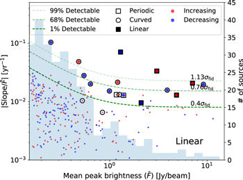
Figure 9. Scatter plot of fractional slope versus mean peak brightness. Background: Histogram of the mean peak brightness for the submillimeter sources as a whole. Small marks indicate the sources of which linear variability are not shown. Three green lines indicate the 99%, 68%, and 1% detectable levels from top. The corresponding values are noted above each line. The red and blue markers indicate the sources with the positive and negative best-fit slopes. Empty circles and squares denote four sources that are only found by sinusoidal fitting (see Figure 3).
Download figure:
Standard image High-resolution imageAs expected, the limiting detectable fractional amplitude varies with source brightness. For the brighter sources, where the measurement uncertainty is dominated by the flux calibration within the map and thus the measurement uncertainty is roughly proportional to the source brightness, the limiting detectable fractional amplitude becomes constant. Once the mean peak submillimeter brightness becomes less than ∼0.5 Jy beam−1, the limiting fractional amplitude increases quickly. Given that the majority of secular variable detections are found within a factor of a few around the limiting threshold while the numbers of protostars increases toward the faint end (see Figure 7), it is clear that the completeness of the survey drops significantly below this brightness limit. The completeness transition can be clearly seen in Table 5. The fraction of secular variables remains about 40% when we limit the sample to bright sources. Once we include sources fainter than ∼0.5 Jy beam−1, however, the fraction of secular variables drops.
Table 5. Variability Detection by Source Brightness
| Condition | S/N | Nsubmm | Nprotostar | Nsecular | Psec a |
|---|---|---|---|---|---|
| (Jy bm−1) | |||||
| ≥0.14 | 10 | 295 | 83 | 18 | 0.22 |
| ≥0.35 | 22 | 141 | 51 | 17 | 0.33 |
| ≥0.5 | 29 | 95 | 43 | 16 | 0.37 |
| ≥1.0 | 41 | 48 | 31 | 11 | 0.35 |
| ≥2.0 | 47 | 45 | 15 | 6 | 0.40 |
Note.
a Fraction of secular variables (Nsecular/Nprotostar).Download table as: ASCIITypeset image
Finally, we caution that the detectable limit varies with region, due to the different number of epochs for each region (see Table 1). In general, this should introduce only minor differences between regions; however, we anticipate a somewhat higher completeness for Serpens Main, where the number of observed epochs is 50% larger than the average over the other regions.
5. Discussion
In Section 3, we found 18 secular variable protostars, out of 83 monitored by the JCMT Transient Survey, and quantified their variability timescales and amplitudes. Next, in Section 4, we established the completeness of our variable sample as a function of source brightness and variability amplitude, determining that for 43 protostars with peak brightness >0.5 Jy beam−1, our sample has a uniform fractional amplitude detection threshold. In this section, we investigate the regional dependency of detected variability, and compare the submillimeter behavior to the known properties of the variables in the literature.
5.1. Variability across Star-forming Regions
Although our survey reveals only a small number of variables, which limits the statistical significance of results from subsamples, we consider possible regional variations in the numbers of secular variables uncovered. Table 6 shows the ratio ( ) between the numbers of secular variables and protostars in each region, to examine any regional dependency. For the full survey, we find 22% of protostars varying, while across the eight individual star-forming regions, we find a wider range: 0%–50%. To account for the completeness (Section 4), we repeat our analysis using only those sources with mean peak brightness greater than 0.5 Jy beam−1 and find that 37% of protostars vary across the entire survey.
Table 6. Detected Variables by Region
| Region | D (pc) | Nproto | Nstch | Nsecular | Psec | pa | Nproto a | Nsecular a | Psec a | pa |
|---|---|---|---|---|---|---|---|---|---|---|
| NGC 1333 | 293 c | 16 | 0 | 3 | 0.19 | 0.75 | 7 | 2 | 0.29 | 0.62 |
| OMC2/3 | 388 d | 14 | 0 | 1 | 0.07 | 0.15 | 12 | 1 | 0.08 | 0.01 |
| NGC 2068 | 388 d | 15 | 0 | 5 | 0.36 | 0.16 | 8 | 4 | 0.50 | 0.42 |
| Serpens south | 436 d | 13 | 1 | 2 | 0.15 | 0.55 | 3 | 2 | 0.67 | 0.28 |
| Ophiuchus cores | 137 d | 9 | 0 | 1 | 0.11 | 0.42 | 1 | 1 | 1.00 | 0.37 |
| Serpens main | 436 d | 8 | 0 | 4 | 0.50 | 0.04 | 7 | 4 | 0.57 | 0.24 |
| IC 348 | 321 d | 5 | 0 | 2 | 0.40 | 0.40 | 3 | 2 | 0.67 | 0.28 |
| NGC 2024 | 423 d | 3 | 0 | 0 | 0.00 | 0.36 | 2 | 0 | 0.00 | 0.28 |
| Whole survey | 83 | 1 | 18 | 0.22 | 43 | 16 | 0.37 | |||
Notes.
a Results when we include only those protostars brighter than 0.5 Jy beam−1. b Region-dependent p-values, obtained from Student's T Test using the ttest_ind task in the stats package of scipy, comparing the fraction of protostellar secular variables in each region against the same fraction over all other regions combined. The test results are null except for Serpens Main, when using all protostars, and OMC 2/3, when limiting to bright protostars (>0.5 Jy beam−1). c Parallaxes from the Gaia DR2 catalog (Ortiz-León et al. 2018). d Parallaxes from the VLBA GOBELINS program (Kounkel et al. 2017; Ortiz-León et al. 2017a, 2017b, 2018).Download table as: ASCIITypeset image
We compare the regional variability ratios by calculating the probability (p) that each region is drawn from an underlying sample with the mean value. Each region is compared against the entire sample, excluding the region of interest. When taking the samples to include all protostars, there is no clear evidence of regional dependence. Serpens Main is somewhat overabundant in variables and has p = 0.04 (P < 0.05 is typically used as a dissimilarity threshold), but has also been most frequently observed and should have a slightly higher completeness threshold than the other regions. Considering only protostars brighter than 0.5 Jy beam−1, where the completeness is more uniform, the OMC 2/3 region becomes somewhat exceptional in harboring fractionally few variables, 1 out of 12 protostars, with p = 0.01. There is no obvious correlation in these numbers with distance to each region. The full set of results is presented in Table 6.
5.2. Variability across Evolutionary Stage
Protostars are expected to be more variable at earlier evolutionary stages. For this analysis, we use the bolometric temperature, corrected for extinction, as a proxy for evolutionary stage. For the three Orion fields, these values were directly obtained from the literature (Furlan et al. 2016). For Serpens, Perseus, and Ophiuchus, bolometric temperature and luminosity values were updated by Mowat (2018) based on the SED-fitting methodology in Dunham et al. (2015) using SCUBA-2 fluxes at 450 and 850 μm from the JCMT Gould Belt survey (Pattle et al. 2015; Chen et al. 2016) to improve the submillimeter coverage. 37
In Figure 10, we plot both the extinction-corrected bolometric luminosities (upper panel) and the peak submillimeter brightnesses (lower panel) of our sample against the extinction-corrected bolometric temperature. We also include the larger Orion HOPS sample (Furlan et al. 2016) in the luminosity panel.
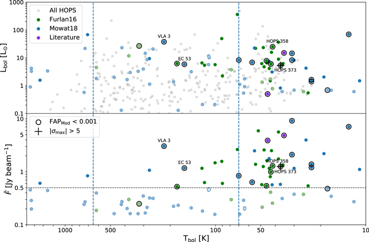
Figure 10. Bolometric luminosity (Lbol, top panel) and mean peak brightness at 850 μm ( , bottom panel) on bolometric temperature (Tbol) space. Green and blue markers denote JCMT Transient Survey sources with physical parameters obtained from the HOPS catalog (Furlan et al. 2016) and Spitzer Space telescope Gould Belt Survey catalogs (Dunham et al. 2015; Mowat 2018), respectively. Purple circles denote two secular variables for which the physical properties were found via a literature search, VLA 1623-243 (Murillo et al. 2018) and CARMA 7 (Maury et al. 2011). Gray markers denote all the sources from HOPS (Furlan et al. 2016). Faint markers denote the sources that are fainter than 0.5 Jy beam−1 (dotted line) at 850 μm. Black circles denote the secular variables, and the black cross denotes the stochastic variable.
Download figure:
Standard image High-resolution imageConsidering just the luminosity versus temperature (upper panel), the protostellar variables are more luminous and cooler than the underlying HOPS sample, but not significantly more luminous than the typical protostar in the JCMT Transient Survey sample. However, in the bottom panel it is clear that peak submillimeter brightness is a strong function of evolutionary class, as expected. Care must be taken before inferring changes in the variability fraction with evolutionary stage due to changing completeness limits as a function of source brightness.
Following the results of Section 4, we consider only those sources for which the mean brightness is greater than 0.5 Jy beam−1, for which the completeness to secular variability is reasonably flat. We thus find 0 (out of 2) Class II secular variables, 3 (out of 10; 30%) Class I secular variables, and 13 (out of 34; 38%) Class 0 secular variables. Although the variability ratio is higher among Class 0 than Class I, the difference between the ratios of Class 0 and Class I is insignificant (p = 0.61).
5.3. Variability of Known Eruptive YSOs
We conducted a literature search for known eruptive variables within the eight JCMT Transient Survey fields. Six such stars were identified across four regions, of which three are coincident with submillimeter peaks. All three of the coincident submillimeter protostars, EC 53 in Serpens Main (also known as V371 Serpentis; Hodapp et al. 2012), V1647 Ori in NGC 2068 (Aspin & Reipurth 2009), and HOPS 383 in OMC 2/3 (Safron et al. 2015) are observed to be varying (see Table 4). Based on bolometric temperature (see Section 5.2), the first two are classified as a Class I while HOPS 383 is a Class 0. The three known eruptive stars for which there is no coincident submillimeter peak are OO Serpentis 38 and V370 Serpentis, both in Serpens Main, as well as IRAS 18270-0153W 39 in Serpens South.
The two optical/IR eruptive (FUOr/EXOr) stars that are found to vary in our submillimeter sample, V1647 Ori and EC 53, are both observed to have episodic accretion outbursts. EC 53 has a short-term, ∼1.5 yr, periodicity, observed at near-IR and submillimeter wavelengths (see, Lee et al. 2020b). V1647 Ori has undergone multiple eruptions, with times between bursts in the 2 to 5 year range (Aspin et al. 2006; Acosta-Pulido et al. 2007; Ninan et al. 2013). Most recently, in 2018, V1647 Ori was observed in a quiescent phase (Giannini et al. 2018). The decrease during 2018 is observed in our survey (see Figure B1.3). The submillimeter light curve for this source is fit with a ∼6 yr period, placing it in the Curved Group. The light curve itself suggests that it may be reaching a minimum (Figure B1.3).
These two known optical/IR eruptive Class I sources are among the most extreme submillimeter variables in our sample in terms of fractional flux change across the observing window. Only HOPS 383, our mid-infrared (MIR) identified eruptive Class 0 variable, along with the three Class 0 sources HOPS 358, HOPS 373, and West 40, reveal a similarly large brightness range (see also Section 5.6). Furthermore, similar to HOPS 383, the three strongly varying Class 0 sources have extrapolated timescales (periods) greater than 8 yr. Interestingly, HOPS 383 has a somewhat lower variability amplitude across the last 4 years, compared with the other three Class 0 variables. This may be due to the fact that its submillimeter brightness decay has recently slowed, after the well-known outburst event between 2004 and 2010 (Safron et al. 2015).
Additional details on each of these protostellar variables can be found in the Appendix.
5.4. Variability of Known Subluminous YSOs
For embedded protostars, their luminosity is dominated by accretion luminosity. Therefore, the low-luminosity sources, which are classified as YSOs with ≤1 L⊙ (Dunham et al. 2008), should have low mass accretion rates. The most extreme low-luminosity sources, called Very Low-Luminosity Objects (VeLLOs), were discovered by the Spitzer survey (Young et al. 2004). By definition, VeLLOs are embedded protostars with the internal luminosity ≤0.1 L⊙, and are thus considered as YSOs in the most quiescent phase of the episodic accretion process. We investigate the variability of low-luminosity sources and VeLLOs revealed in submillimeter.
First, we cross-matched those low-luminosity sources from Dunham et al. (2008) with the source list in this study. We note that the SMM 1 was classified as a low-luminosity source by Dunham et al. (2008) using the 2MASS and Spitzer data set (1.25–70 μm). 40
There are 28 low-luminosity sources located within our coverage, with seven LLSs brighter than >0.14 Jy beam−1 at 850 μm: two in IC 348, four in NGC 1333, and one in Ophiuchus. The two low-luminosity sources in IC 348, MMS 1 and HH 211, are secular variables (Figures B1.1 and B1.8). Thus, two out of seven low-luminosity sources (∼30%) show secular variability in the submillimeter. Comparing this variability fraction against the entire sample of monitored protostars (see Table 6), we obtain a p-value of 0.69. For the sources F80% > 0.5 Jy beam−1, the number of variables from the sample becomes two out of four (50%), for which the p-value is 0.59. Thus, we do not detect any clear differentiation in the secular variability fraction of low-luminosity sources, with any conclusions limited by the small sample size.
As an alternate sample, we compare our source list to the VeLLO list from Kim et al. (2016). Kim et al. (2016) added four complementary criteria (a ratio of the 1.65 μm flux to the 70 μm flux less than 2.8; a 4.5 μm magnitude brighter than 15.3; not being registered as galaxies in known databases; and a color index [8]–[24] > 2.2) from Dunham et al. (2008) for identifying VeLLOs. Only four VeLLOs from this sample, all in the Serpens South region, are detected in the submillimeter, although 14 VeLLOs (one in IC 348, two in NGC 1333, two in Ophiuchus, and nine in Serpens South) are within our coverage. None of the matched VeLLOs shows secular variability in our analysis. Despite the null detection of variability among these four observed VeLLOs, there is no evidence that the small VeLLO sample is different than the larger survey sample. That is, comparing the fractional variability within the VeLLO sample against the larger survey sample yields a p-value ≈0.14, well above the 0.05 typically used to justify differences in the samples.
5.5. Comparison with NEOWISE Variables
According to our results, submillimeter continuum emission traces only variability in protostellar luminosity, which appears as a temperature change in the thick envelope. Optical and near-IR brightness variations are sensitive to the luminosity, but may also be caused by extinction changes within the small inner region close to the central object, (i.e., optical depth to the stellar photosphere and inner disk). As a corollary, the variability of YSOs at later evolutionary stages, without much remaining envelope, is primarily revealed at shorter wavelength. Furthermore, different physical and geometrical scales associated with underlying variability processes also determine the timescales of variability.
In this sense, the MIR covers a wider range of physical/geometrical scales, and thus, a greater variety of variability mechanisms than are expected to be traced in the submillimeter. An intensive investigation for YSO variability in the MIR has been undertaken for ∼5400 YSOs in 20 nearby low-mass star-forming regions, using NEOWISE W2 band (4.6 μm) light curves covering ∼7 years (Park et al. submitted). Here, we compare the JCMT Transient Survey results to that MIR variability investigation.
In total, 1204 NEOWISE sources are located within our eight Transient survey regions. Of those, 49 have submillimeter counterparts: 39 are classified as protostars, 9 are disk sources, and 1 submillimeter peak is coincident with a Class III or evolved source. For the protostars in common, 23 out of 39 (59%) are variables in the MIR over the 6.5 years monitored by NEOWISE, very similar to the 55% variability likelihood over all protostars detected by that survey (W. Park et al. submitted).
From our survey, 8 submillimeter protostellar variables have counterparts observed in the W2 band, yielding a 20% (8 out of 39) variability rate almost identical to the likelihood over the full submillimeter survey. Five of these sources are identified as variable at both wavelengths. West 40, V1647 Ori, and Serpens Main-SMM 1 are classified as Curved in both submillimeter and MIR. EC 53 and Serpens Main-SMM 10 are varying in W2 but classified as MIR irregulars, which means no notable secular trend in the W2 light curves. HOPS 389, NGC 1333-VLA 3, and SH 2-68-N are not observed to vary in the MIR.
Similar to the submillimeter analysis in this work, Park et al. (submitted) classified the YSO MIR variability largely into two categories, i.e., secular and stochastic. As here, they further divided secular variability into three types: Linear, Curved, and Periodic; however, the boundary between the groups is different because of the different cadences and coverage in the two surveys. Given the large number of MIR stochastic variables that they found, they further divided the stochastic variability into three types: Burst, Drop, and Irregular. Burst and Drop are identified by sudden brightening and dimming only in a few epochs (i.e., with short timescales) over the 7 yr light curve, while Irregular is identified by the random distribution of brightness with a high standard deviation, in which no underlying timescale of variability is measured.
The distinct difference between protostellar variability observed in the MIR versus the submillimeter is that most of the MIR variability is irregular while all variables in the submillimeter show secular trends. This difference can be interpreted in terms of both the different cadences of observations and the different origins for the variability at these two wavelengths. The cadence of NEOWISE is about 6 months, but that of the JCMT Transient Survey is typically one month or shorter. As a result, periodic MIR variability with a short period is more likely to be classified as irregular variability for the NEOWISE light curves. EC 53 provides a good example; it is classified as an irregular variable in the MIR, but as a periodic variable in the submillimeter. The period of EC 53 is about 1.5 yr. However, the periodogram analysis in the MIR (W. Park et al. submitted) did not find it as a periodic source because the light curve is not simply sinusoidal (see Figure 1 and Lee et al. 2020b), and the MIR data cadence is too sparse to pull out the periodicity.
There is an additional explanation for the significantly larger numbers of observed irregular variables in the MIR compared with the submillimeter. MIR brightness is intrinsically sensitive to the variability of the protostar, while the submillimeter radiation is sensitive only to the variability of the envelope temperature, where the submillimeter emission arises. As a result, stochastic changes in the accretion luminosity or extinction events taking place close to the central source can be more easily detected in the MIR. Sudden changes in accretion luminosity, however, are smoothed by the large envelope, given its long thermal relaxation time of a month or longer (Johnstone et al. 2013), and the fractional change in submillimeter flux, which is proportional to the temperature change, is lowered by a factor of ∼5.5 compared to that in MIR (Contreras Peña et al. 2020).
Finally, there are no epochs in which the observed submillimeter emission becomes much lower, i.e., drops, for a single epoch. In the MIR sample, a non-negligible number of disk sources show such short-timescale behavior. The lack of dips in the submillimeter is most likely due to the fact that the observed submillimeter radiation emitted by the envelope traces the time-averaged luminosity of the source, where the averaging is over the months of thermal equilibrium time of the radiating envelope (see Johnstone et al. 2013). Thus, while it is possible that a nonthermal brightening event such as a flare (Mairs et al. 2019) might add to this emission to produce a burst, there are no short-timescale subtractions of emission. Furthermore, the submillimeter radiation from the envelope is optically thin, and thus responds only linearly to changes in optical depth, unlike the optical through MIR where small changes in the line-of-sight column density can provide very large optical depth variations and strong dimming on a variety of timescales.
5.6. Variability as a Proxy for Episodic Mass Accretion
A key result from four years of monitoring protostars in the submillimeter is that at least 20% are seen to undergo secular variations in their brightness. The fraction rises to 40% when only the brighter protostars are included in the sample. Nevertheless, the measured fractional variability amplitudes and slopes for individual sources (see Table 4, columns 6 and 7) appear to be modest, and thus one might be tempted to dismiss the observed variability as physically unimportant with respect to the mass assembly process for protostars. However, as noted by Johnstone et al. (2013), the submillimeter emission reacts to the temperature of the protostellar envelope, effectively probing the Rayleigh–Jeans tail of the Planck curve, and thus converting the observed variability to the underlying protostellar brightness variations requires a significant, exponential boost (see also MacFarlane et al. 2019a, 2019b). Through comparison of observed variables at both MIR and submillimeter wavelengths, Contreras Peña et al. (2020) empirically uncovered a submillimeter-to-protostellar luminosity exponential factor of ∼4, and confirmed that it matched well with radiative transfer expectations (Baek et al. 2020). Thus, assuming that the protostellar luminosity is a reasonably linear proxy for protostellar accretion, it is appropriate to consider the importance of the variable mass accretion uncovered by these submillimeter observations.
We begin by assuming that the 12 secular variables best fit with periodic light curves undergo bursts with duration timescales half the measured period and burst amplitudes equal to twice the amplitude, Aburst = 2 × A (see Table 4), effectively requiring that quiescence is determined at the lowest point on the observed light curve. Furthermore, for those six variables best fit by linear slope measurements, we assume that the burst takes place during half of the observing window, ∼2 yr, and that the burst amplitude is four times the (yearly) slope, Aburst = 4 × Slope (see Table 4). This latter assumption is likely a significant underestimate of the importance of the burst, as we are constraining the amplitude by the observing time window.
With these estimates for the submillimeter burst strength, we can now directly compute the excess amount of mass accreted during each burst after subtraction of the quiescent mass accretion, Mburst, against the total mass that is accreted at the fixed quiescent rate over the full time period, Mquiescent:

Thus, a null value refers to no variability, Aburst = 0, whereas a very powerful burst would add many multiples of the quiescent accreted mass. For the quantities tabulated in Table 4, we find that the smallest amplitude variables add ∼10% of the quiescent accreted mass (integrated over the full time range) through their years-long burst enhancement. The six most prominent variables, however, each add greater than 40% during the burst phase.
Using this simple model, the most powerful burst accretor in our sample is V1647 Ori, adding an additional 125% of the quiescently accreted mass during each ∼3 yr burst. Furthermore, during each burst V1647 Ori attains a peak mass accretion rate 3.5 times the quiescent rate,

Similarly, EC 53 (V371 Ser) adds an additional 60% of the quiescently accreted mass during each of its ∼ 0.75 yr bursts, attaining a peak burst mass accretion rate twice the quiescent rate. As noted in Section 5.3, both of these known Class I repeaters belong to the FUOr/EXOr type of eruptive stars and have repetition timescales in the literature similar to what is determined in our analysis.
In addition to EC 53 and V1647 Ori, four Class 0 protostars in our sample have measured high amplitude variability and associated large burst accretion rates: HOPS 356 (85%), HOPS 373 (70%), West 40 (45%), and HOPS 383 (40%) (see Table 4). All of these sources are associated with long timescales, periods of at least twice the 4 yr monitoring window, and thus the measured amplitudes and burst accretion rates are anticipated to be lower limits.
The simple analysis presented in this section suggests that the mass assembly of protostars can be significantly influenced by bursts on timescales of years. Roughly 7%, 6 out of the 83 monitored protostars, show order unity mass accretion variability on this timescale. Assuming that all protostars sample the range of variability observed by our sample, we predict that, for a given source, years-long bursts occur on average about every ∼50 yr. Thus, the importance of these accretion events for the overall mass assembly of the typical protostar is not large, accounting for only a few percent of the accreted mass.
The results presented here are in contrast to the extreme bursting events searched for in the MIR by Scholz et al. (2013) and Fischer et al. (2019), where less than 1% of the protostars were seen to vary on timescales of half a decade, implying an underlying random distribution of extreme bursts for a given source with ∼1000 yr between each event. There remains a vast unexplored time domain separating these two extremes for episodic mass accretion that warrants detailed investigation. This will require continued searches for rare brightening events as well as dedicated monitoring of protostellar samples in order to determine if the variability uncovered in this paper smoothly connects with the rarer but more extreme events or if the variability separates cleanly into well-defined episodic timescales. Both possibilities would yield significant constraints for theoretical models of mass accretion, both steady-state and unstable, through the disk.
Finally, we note that continued monitoring in the submillimeter is essential for the youngest, most embedded, protostars. The four strongly varying Class 0 sources identified here, with variability amplitudes similar to the known eruptive systems EC 53 and V1647 Ori, are hard to interpret from MIR observations alone, due to the extreme extinction of the central source and disk (see, e.g., the multiwavelength analysis of HOPS 373 by Yoon et al. in prep.). ALMA observations are also revealing complicated geometries during these very early phases of protostar evolution, such as multiple protostars and an arc-like structure within an extremely dense and compact core (Tokuda et al. 2014) and multiple misaligned outflows from a single young protostar (Okoda et al. 2021). The explanation for these features is assumed to be complex gas accretion within a turbulent core. Such complex structure will inevitably produce protostellar accretion variability. It will, therefore, be important to also study the relation between submillimeter variability and the small-scale structure near the protostar using high spatial resolution observations such as by ALMA.
6. Conclusions
In this paper, we have analyzed four years of JCMT Transient Survey (Herczeg et al. 2017) monitoring of 295 (95) submillimeter peaks, >0.14 Jy beam−1 (>0.5 Jy beam−1), of which 83 (43) are protostellar. We analyzed the light curves by searching for and statistically quantifying single-epoch events, long-term monotonic trends by fitting linear functions, and long-term nonlinear trends or periodicity by fitting sinusoidal functions with the Lomb–Scargle periodograms. Although the light curves are more complicated and most variables are not fit well with any single function, these fits provide uniform statistical results that reasonably describe the size and timescale of the measured variability. Eighteen of 83 protostars are variable with a secular trend and are classified as Periodic, Curved, or Linear by their best-fit periods. No robust single-epoch events or sources with indefinite stochastic trends across the time coverage are detected for these bright sources.
To evaluate sensitivity limits for our ability to detect changes with different amplitudes and timescales, we performed a completeness analysis for secular variability, taking into account source brightness, measurement uncertainty, variability timescale, and fractional amplitude of the variation. The sensitivity of the survey to variability mainly depends on the source brightness, and becomes uniform for the sources brighter than 0.5 Jy beam−1. Following this result, we expect to find more secular variables from our extended survey as the time coverage extends, making it easier to observe secular trends. Additionally, efforts to improve the relative calibration between epochs from ∼2% to ∼1%, should also significantly increase the number of variables recovered by our analysis techniques. Across the eight regions monitored by the survey, the sample of sources brighter than 0.5 Jy beam−1 in OMC 2/3 region show a statistically significant low variable fraction compared against the other regions. No other region showed significant evidence for regional variation. The evolutionary dependency of variability only showed marginal evidence for more episodic sources in Class 0 versus Class I for our sample.
We compared the variability properties of the known eruptive and subluminous YSOs within our sample. Three eruptive YSOs identified previously in the optical, NIR, or MIR, V1647 Ori, EC 53 (V371 Ser), and HOPS 383, robustly vary in the submillimeter. We note that an additional three Class 0 sources showing strong submillimeter variability, HOPS 373, HOPS 356, and West 40, should continue to be monitored for potential powerful eruptions. Somewhat unexpectedly, the subluminous sample of YSOs shows no evidence of a different variability behavior compared against the eruptive sources.
Finally, using a simple model to convert submillimeter variations to underlying mass accretion variability, we find that all of the secular variables uncovered by the JCMT Transient Survey require significant enhancement, greater than 10%, in mass accreted due to bursts versus quiescence. For the six most variable sources, 7% of our sample, we find that the accreted mass due to the burst alone is greater than 40% and reaches more than 100%. When integrated over the full protostellar ensemble, the importance of episodic accretion on these few years timescale is negligible, only a few percent of the assembled mass. However, the measured variability is dominated by events on the order of the observing time window on a relatively small sample of objects. Continued submillimeter monitoring of these fields and of intermediate-mass star-forming regions with more ongoing star formation is needed to reveal the importance of episodic events on decades and longer timescales.
We thank the anonymous referee for the helpful comments on our paper. The authors wish to recognize and acknowledge the very significant cultural role and reverence that the summit of Maunakea has always had within the indigenous Hawaiian community. We are most fortunate to have the opportunity to conduct observations from this mountain.
The James Clerk Maxwell Telescope is operated by the East Asian Observatory on behalf of The National Astronomical Observatory of Japan; Academia Sinica Institute of Astronomy and Astrophysics; the Korea Astronomy and Space Science Institute; the Operation, Maintenance and Upgrading Fund for Astronomical Telescopes and Facility Instruments, budgeted from the Ministry of Finance (MOF) of China and administrated by the Chinese Academy of Sciences (CAS), as well as the National Key R&D Program of China (No. 2017YFA0402700). Additional funding support is provided by the Science and Technology Facilities Council of the United Kingdom and participating universities in the United Kingdom and Canada. Additional funds for the construction of SCUBA-2 were provided by the Canada Foundation for Innovation. The James Clerk Maxwell Telescope has historically been operated by the Joint Astronomy Centre on behalf of the Science and Technology Facilities Council of the United Kingdom, the National Research Council of Canada, and the Netherlands Organisation for Scientific Research.
This research used the facilities of the Canadian Astronomy Data Centre operated by the National Research Council of Canada with the support of the Canadian Space Agency. This research has made use of the SIMBAD database, operated at CDS, Strasbourg, France (Wenger et al. 2000).
D.J. is supported by NRC Canada and by an NSERC Discovery Grant. J.-E.L. is supported by the National Research Foundation of Korea (NRF) grant funded by the Korea government (MSIT) (grant number 2021R1A2C1011718). G.J.H. is supported by general grant 11773002 awarded by the National Science Foundation of China. The contribution of C.C.P. was funded by a Leverhulme Trust Research Project Grant. G.B. was also supported by the National Research Foundation of Korea (NRF) Grant funded by the Korean Government (NRF-2017H1A2A1043046-Global Ph.D. Fellowship Program). D.H. acknowledges support from the EACOA Fellowship from the East Asian Core Observatories Association. G.P. is supported by the Basic Science Research Program through the National Research Foundation of Korea (NRF) funded by the Ministry of Education (NRF-2020R1A6A3A01100208). P.S.T. acknowledges support from YSTFC grant ST/R000824/1. J.B. acknowledges support by NASA through the NASA Hubble Fellowship grant #HST-HF2-51427.001-A awarded by the Space Telescope Science Institute, which is operated by the Association of Universities for Research in Astronomy, Incorporated, under NASA contract NAS5-26555. F.D. is supported by the National Natural Science Foundation of China through grant 11873094. H.S. acknowledges support from the Ministry of Science and Technology (MoST) of Taiwan through grant109-2112-M-001-028-. D.S. recognizes support from STFC grants ST/N504014/1 and ST/M000877/1. S.P.L. acknowledges grants from the Ministry of Science and Technology of Taiwan 106-2119-M-007-021-MY3 and 109-2112-M-007-010-MY3. Y.A. acknowledges support by NAOJ ALMA Scientific Research grant Numbers 2019-13B, Grant-in-Aid for Scientific Research (S) 18H05222, and Grant-in-Aid for Transformative Research Areas (A) 20H05844 and 20H05847. S.-P.L. acknowledges grants from the Ministry of Science and Technology of Taiwan 106-2119-M-007-021-MY3 and 109-2112-M-007-010-MY3.
Software: makemap (Chapin et al. 2013), STARLINK (Currie et al. 2014), SMURF (Jenness et al. 2013), Astropy (Astropy Collaboration et al. 2013), SciPy (Virtanen et al. 2020), Matplotlib (Hunter 2007)
Appendix A: Derivation of Detectable Amplitude with χ2
Assume that a source varies as a sinusoid with  , where A, ω, and ϕ0 are the amplitude, frequency, and initial phase of the sinusoidal function, respectively, and F0 is constant. Considering N observations taken at fixed times and with fixed measurement uncertainties, the analytic definitions of χ2 under two hypotheses, the sinusoidal function (
 ) and a constant, or null, function (
 ), are then
where Gi
(σfid) is the Gaussian error of ith epoch, Xi
= 2π
ω
ti
+ ϕ0,  , and
, and  is the mean value of F(t) over the observations.
Expanding the null solution, one obtains three terms with varying powers of A,
Thus,  can be written in the form of a quadratic equation depending on A such that

where
We further note that the last term, T3, is equivalent to  .
.
The ratio of the χ2 terms determines the power of the best-fitting sinusoid (Equation (1)) as well as the false alarm probability (Equation (2)). Thus, we obtain
where we make the assumption that  is small.
In our analysis, we consider a source robustly detected when  therefore, we can solve Equation (A5) for
  :
:

We thus set  and remembering that
  is equal to T3, we substitute Equation (A6) into Equation (A3) to obtain the inequality

This equation can be solved for the minimum detectable amplitude as a function of sinusoidal properties, measurement times, and measurement uncertainties. The minimum detectable amplitude,  , is therefore
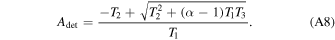
We use a Monte Carlo approach to solve for the T1, T2, and T3 terms in Equation (A4) under observing conditions similar to those in our survey and for sinusoids with fixed periods and random phases. The results are presented in Figure A1. Each point indicates a detectable amplitude of a hypothetical light curve. The phase dependency of detectable amplitude appears as spike-shaped features in the left panel. In short, for sinusoids with long periods, it is difficult to distinguish the underlying signal when the source is near minimum or maximum amplitude and the light curve is relatively flat over the observing window. We sum over the various phases to determine the completeness threshold as a function of period. The period dependency of the detectable amplitude is indicated by the histogram in the right panel, which shows that the detectable amplitudes of short-period sources become concentrated around the value of σ derived above.
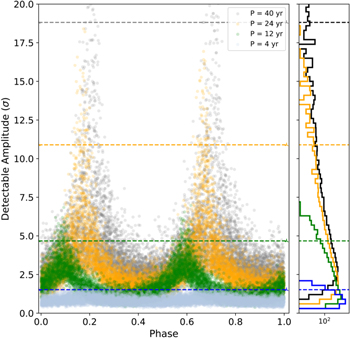
Figure A1. The detectable amplitude in σfid level depends on phase. The different colors indicate the different periods of the hypothetical signals. For the longer periods, the spikes in a certain phase become sharper and higher. Right panel shows the histogram of the detectable amplitude. The colored dashed lines in both panels denote the 99% detectable level of each corresponding period.
Download figure:
Standard image High-resolution imageFurthermore, we derive the minimum detectable amplitude under an ideal assumption of a sinusoid observed well enough in time to provide uniform phase coverage. This is most likely to occur for sources with periods shorter than the observing window. We can then treat the summation of the coefficients as T1 = N/2, T2 = 0, and  , where
  is the expected uncertainty for a given measurement. Under these simplifications, Equation (A8) reduces to

where the amplitude of the minimum detectable periodic signal is proportional to the measurement uncertainty.
We can apply the same sequence of steps to determine the required slope a of a robustly detected linear function. Here, the two χ2 are
Expanding  , we obtain
Following Equation (A5), for the linear hypothesis, we obtain
where, for a robust detection, we require FAPLin < 10−3. Therefore,

Appendix B: Detected Variables as Individual Cases
In this appendix, we note the information derived from literature searches about each of all the identified secular (Table 4) variables. The light curves in Figure Set B1 are available in the online material.
B.1. Perseus IC 348, MMS1: Periodic Group
The submillimeter light curve for secular source Perseus IC 348, MMS 1 is presented in Figure B1.1. The JCMT source is associated with a millimeter peak with a separation of 0 66 from the Class 0 protostar IC 348 MMS. Continuum observations by by Chen et al. (2013) with the SMA established IC 348 MMS as a multiple system, with two continuum sources, MMS1 and MMS2, embedded in a common envelope and separated by 98. IC 348 MMS1 drives molecular outflow traced in H2 (Eislöffel et al. 2003) with distinct red and blueshifted lobes detected in CO (Lee et al. 2016). Additionally, Segura-Cox et al. (2016) identified MMS1 as a disk candidate in the VLA Nascent Disk and Multiplicity (VANDAM) Survey. The second continuum source, MMS2, is potentially a protobinary confirmed by presence of an outflow, HH797, with signatures of a rotating jet (McCaughrean et al. 1994; Pech et al. 2012).
B.2. Serpens Main EC 53 (V371 Serp): Periodic Group
The submillimeter light curve for secular source Serpens Main EC 53 (V371 Serp) is presented in Figure B1.2. Based on its bolometric temperature and spectral index, EC 53 is a Class I source (Evans et al. 2009; Dunham et al. 2015). However, the envelope contains ∼6 M⊙ (Baek et al. 2020), while the protostar and disk masses are only 0.3 M⊙ and 0.07 M⊙, respectively (Lee et al. 2020a), suggestive of a much younger evolutionary state. Periodic variability has been observed previously in the near-IR (Hodapp 1999; Hodapp et al. 2012), MIR (Contreras Peña et al. 2020), and the submillimeter (Mairs et al. 2017b; Yoo et al. 2017; Johnstone et al. 2018). Deep CO and H2O absorption lines, indicative of viscous disk heating and characteristic of FUOrs, are also observed (Connelley & Reipurth 2018). Lee et al. (2020b) combine these observations across wavelengths to analyze the physical process responsible for each burst.
B.3. Orion NGC 2068, HOPS 389: Curved Group
The submillimeter light curve for secular source Orion NGC 2068, HOPS 389 is presented in Figure B1.3. Launhardt et al. (1996) observed this source in the 1.3 mm continuum using the IRAM 30 m telescope, finding it to have a compact condensation with more extended envelope. The presence of two embedded infrared sources led to its identification as a self-luminous protostellar core (Class 0/I). Mitchell et al. (2001) mapped the source using SCUBA and weakly detected an associated outflow in 12CO 3–2. Walker-Smith et al. (2013) also observed patches of red- and blueshifted 13CO 3–2 emission in the vicinity of this source. Matthews & Wilson (2002), using the SCUBA polarimeter, found the polarization toward the source to be consistent with that of its surroundings.
Spezzi et al. (2015) list one source for these coordinates, classified as Class I based on the SED slope between 2.2 and 24 μm. Furlan et al. (2016) find two closely associated sources, HOPS 323 and 389, classifying HOPS 323 as Class I and HOPS 389 as Class 0. Here, we identify the submillimeter source with HOPS 389, although HOPS 323 is somewhat more luminous. Both sources are listed as protostars in the Spitzer survey of YSOs in Orion (Megeath et al. 2012). These two objects, together with HOPS 322, are described as a group of protostars.
The VLA/ALMA Nascent Disk and Multiplicity (VANDAM) Survey of Orion Protostars (Tobin et al. 2020) detected four localized 870 μm sources, presumed to be disks: HOPS-323-A at 05:46:47.697 + 00:00:25.27 (44.475 ± 0.754 mJy) and HOPS-323-B at 05:46:47.667 + 00:00:24.81 (81.351 ± 1.484 mJy), both Class 1; and HOPS-389-A at 05:46:47.019 + 00:00:27.07 (19.722 ± 0.668 mJy) and HOPS-389-B at 05:46:46.604 + 00:00:29.52 (4.785 ± 0.325 mJy), both Class 0.
B.4. Perseus NGC 1333, IRAS 4A: Curved Group
The submillimeter light curve for secular source Perseus NGC 1333, IRAS 4A is presented in Figure B1.4. The bright infrared (Dunham et al. 2015) through submillimeter (Kirk et al. 2006; Enoch et al. 2009) source is classified as Class 0. IRAS 4A is resolved as a double source by Tobin et al. (2016a) and appears to harbor a massive disk ∼1 M⊙ (Tychoniec et al. 2018) and a large-scale bipolar molecular outflow (Choi 2001). The source was monitored by Spitzer at 3.6 and 4.5 μm for ∼35 days as part of YSOVAR (Rebull et al. 2015), but was not found to be variable in the MIR.
B.5. Serpens Main, SMM 10: Curved Group
The submillimeter light curve for secular source Serpens Main, SMM 10 is presented in Figure B1.5. The source has been identified as Class I (Kryukova et al. 2012), and is also known as Ser-emb-12 (Enoch et al. 2009). Near-infrared K-band observations have identified a stellar counterpart to the submillimeter source, SMM 10 IR, which is found to vary by about 2 mag in K band, and is associated with a fan-shaped nebulosity (Hodapp 1999). Correlated secular variability on year-to-year timescales is found for both MIR NEOWISE and Transient Survey submillimeter observations of the source (Contreras Peña et al. 2020). ALMA 12 m array band 6 observations (Project ID: 2013.1.00618.S; ALMA source name: 211) of the dust continuum at 094 resolution reveal the source to be a binary, with a separation of 425, hosting a complex outflow structure in the 12CO line.
B.6. Ophiuchus Core, VLA 1623-243: Curved Group
The submillimeter light curve for secular source Ophiuchus Core, VLA 1623-243 is presented in Figure B1.6. VLA 1623-243 comprises three protostars: VLA 1623 A, an embedded Class 0 source 56 from the peak of 850 μm emission; VLA 1623 B, a Class 0 source 65 from the peak; and VLA 1623 W, a Class I YSO that is much farther away, with projected distance of 160 (Ward-Thompson et al. 2011; Murillo & Lai 2013). VLA 1623 A and B are just 12 apart, and thus cannot be resolved by the JCMT. We therefore associate the binary system with the observed submillimeter light curve, although VLA 1623 A is brighter (Murillo et al. 2018) and thus expected to contribute most to the observed flux. VLA 1623 A has an envelope mass ∼0.8 M⊙ (Murillo et al. 2018), a disk with an outer radius of 180 au traced by C18O emission (Murillo et al. 2013), and a large-scale bipolar outflow (Santangelo et al. 2015). VLA 1623 B is a weaker source with about a quarter of the envelope mass of that surrounding VLA 1623 A (Murillo et al. 2018). Santangelo et al. (2015) also found a smaller strongly collimated outflow associated this component. Interestingly, VLA 1623 B was determined to be variable at centimeter wavelengths by Coutens et al. (2019).
B.7. Orion NGC 2068, V1647 Ori: Curved Group
The submillimeter light curve for secular source Orion NGC 2068, V1647 Ori is presented in Figure B1. V1647 Ori is the only viable target that is close to the observed submillimeter peak. It is classified as FUOr-like (Connelley & Reipurth 2018) with multiple bursts: 2003, 2008, and 2011 (Aspin et al. 2006; Acosta-Pulido et al. 2007; Ninan et al. 2013; Giannini et al. 2018). The source was reported to dim in July 2012 by Ninan et al. (2012), four years before the start of the JCMT Transient Survey. Its classification, based on the spectral energy distribution, changes over time, but recent work (Furlan et al. 2016) classifies it as a Class I source in transition to Class II with a flat spectrum. Andrews et al. (2004) reported an increase of a factor of 25 at 12 microns and an order-of-magnitude increase in bolometric luminosity up to 34 L⊙. In the quiescent phase, Ábrahám et al. (2004) approximate V1647 Ori's luminosity around 5–6 times solar.
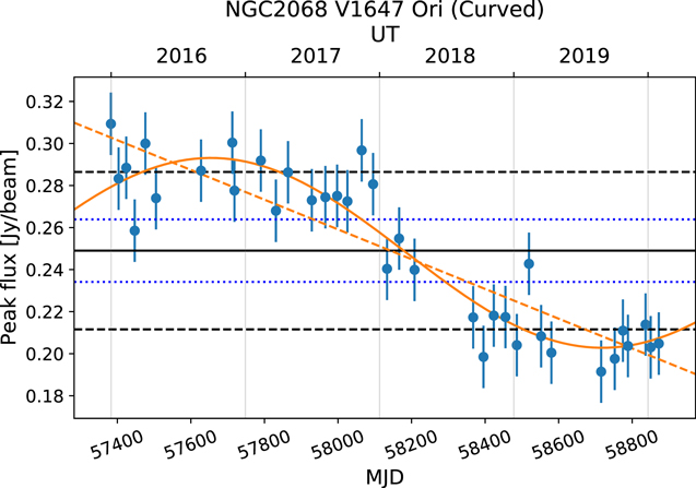
Figure B1.
Light curve of the identified variable source, V1647 Ori in NGC 2068. Black solid line indicates the mean peak brightness in Jy beam−1. Black dashed line and blue dotted line indicate the observed standard deviation and fiducial error from the mean peak brightness, respectively. The orange solid line denotes the sinusoidal fitting provided by LSP, while the orange dashed line denotes the linear fitting result. Both the linear and sinusoidal fits are robust, FAP <0.1%. See Tables 3 and 4 for details. (The complete figure set (18 images) is available.)
Download figure:
Standard image High-resolution imageUsing VLTI, Ábrahám et al. (2006) found no companion around V1647 Ori. There is a possible flared disk around V1647 Ori with a disk mass of 0.05 M⊙ as inferred from MIR. Mosoni et al. (2013) modeled the MIDI observations toward this source and found that the disk+envelope pre- and post- burst structures are similar. With the recent ALMA observations, Cieza et al. (2018) constrain the target to a 40 au disk whose mass is 80 Jupiter masses and with an inclination of 57°. They did not include the envelope model in this case. The earliest jets observations were obtained by Eisloffel & Mundt (1997). A molecular CO outflow was later detected by Andrews et al. (2004). From infrared imaging, the outflow direction is north to south with respect to the source.
The long-term evolution of this source up to 2006 is reported by Acosta-Pulido et al. (2007). The I-band magnitude dropped by 5 magnitude from 2004 February to 2006 January, with a rapid drop at the end of 2005. A periodicity of 56 days was determined from the long-term decay that can be explained by dust structures as indicated by Eiroa et al. (2002). A high-cadence photometry reported by Bastien et al. (2011) uncovered flickers that may be due to interactions between the magnetosphere and the disk. Aspin (2011) reported a new flare in 2011 with a total luminosity of 16 L⊙ and an accretion rate of 4 × 10⁻⁶ M⊙ yr−1, which is similar to the earlier flare in 2004 (Fedele et al. 2007).
B.8. Perseus IC 348, HH 211: Secular Source
The submillimeter light curve for secular source Perseus IC 348, HH 211 is presented in Figure B1.8. The JCMT peak coincides with the dense core HH 211. This continuum source comprises two respective embedded sources, HH 211 SMM1 and HH 211 SMM2, with an angular separation of 031 resolved by high-resolution observations with the SMA (Lee et al. 2009; Chen et al. 2013).
HH 211 SMM1 is an embedded young Class 0 protostar object, potentially the youngest in Perseus (Hirota et al. 2008). It is the exciting source (Avila et al. 2001) for a highly collimated jet observed in H2 (McCaughrean et al. 1994) and SiO (Hirano et al. 2006). Furthermore, Gueth & Guilloteau (1999) detected molecular outflow activity in CO, with low-velocity CO emission tracing bipolar cavities and high-velocity emission aligned with the collimated jet-like structure closer to the central object. Lee (2020) notes that the knots of emission in the jet have estimated timescales between decades and centuries. The central source appears as a flattened disk-like structure, with a size ∼80 au, inclined perpendicular to the jet and outflow axis (Gueth & Guilloteau 1999; Lee et al. 2009).
Wiseman (2001) uncovered a rotating envelope in ammonia emission, normal to the outflow and very close to the central protostar. Additionally, Tanner & Arce (2011) and Tobin et al. (2011) detected notable line broadening indicative of outflow–envelope interaction using ammonia observations. High-resolution mapping with ALMA, by Lee et al. (2018), confirmed the presence of a disk and found small outflow velocities indicating a rotating disk atmosphere. Properties of the adjacent continuum source, SMM2, which has a lower mass than SMM1, are mostly uncertain.
B.9. Orion NGC 2068, HOPS 315: Curved Group
The submillimeter light curve for secular source Orion NGC 2068, HOPS 315 is presented in Figure B1.9. HOPS 315 is classified as a Class I protostar via SED fitting by Furlan et al. (2016). Könyves et al. (1919) identified a dense core 36 away from our JCMT peak using PACS and SPIRE images from the Herschel Gould Belt survey. The authors derived a critical Bonnor–Ebert mass ratio of 0.2 for the core, indicating that it is self-gravitating. Recently, Tobin et al. (2020) used ALMA 870 μm observations to derive protostellar disk properties, including the dust disk radius ∼46 au and dust disk mass ∼100 Earth masses. Kounkel et al. (2016) found no companions within 100–1000au of HOPS 315 using near-IR observations. ALMA observations of the source and outflow are also presented by Dutta et al. (2020).
B.10. Orion NGC 2068, HOPS 373: Curved Group
The submillimeter light curve for secular source Orion NGC 2068, HOPS 373 is presented in Figure B1.10. Gibb & Little (2000) identified this source as a Class 0 protostar, and mapped a bipolar outflow with high-velocity dense gas. The geometric center of this outflow was close to the position of a previously detected H20 maser (Haschick et al. 1983). Edwards & Snell (1984) had previously detected high-velocity molecular gas in the vicinity of the maser. Phillips et al. (2001) observed the source with SCUBA and found its 450 μm emission to be elongated perpendicular to the outflow direction. In CARMA 2.9 mm continuum imaging (Tobin et al. 2015), the source appears to be a binary. The outflow was further studied with CARMA (Tobin et al. 2016b), and a compact second component with the opposite orientation was seen, perhaps due to a second outflow from the binary source. From the (Herschel PACS) O I (63.18 μm) line intensity, they estimate a mass-loss rate of 1.1 × 10⁻⁷ M⊙ yr−1.
The VLA/ALMA Nascent Disk and Multiplicity (VANDAM) Survey of Orion Protostars (Tobin et al. 2020) detected two 870 μm sources, presumed to be disks: HOPS-373-A at 05:46:31.099-00:02:33.02 (103.827 ± 1.626 mJy) and HOPS-373-B at 05:46:30.905-00:02:35.19 (92.206 ± 0.947 mJy), classifying both as Class 0.
The JCMT Gould Belt Survey (Kirk et al. 2016) did not find an associated protostar in the Spitzer (Megeath et al. 2012) or Herschel (Stutz et al. 2013) survey catalogs of YSOs in Orion. However, the source is included in the second paper on the Spitzer Orion survey (Megeath et al. 2016) as a newly Spitzer-identified YSO (there classified as disk) and later listed by Stutz et al. (2013) as a PACS Bright Red source (PBRS).
The source was observed using the SCUBA polarimeter by Matthews & Wilson (2002), and while polarization was seen along the filament where it is located, no polarization was detected toward the source itself. The authors suggest that this end of the filament may lie in the foreground of the nebula, as do Walker-Smith et al. (2013).
Kang et al. (2015) find a high deuteration ratio (HDCO/H2CO) for this source, implying that it is probably in the very earliest stage of star formation. Its classification as a PBRS also argues for it being a very young protostar, and this is corroborated by the models of Furlan et al. (2016). However, Tobin et al. (2015) found rapidly declining visibility amplitudes and suggest it may be slightly more evolved.
B.11. Orion A OMC2/3, HOPS 383: Curved Group
The submillimeter light curve for secular source Orion Orion A OMC2/3, HOPS 383 is presented in Figure B1.11. Safron et al. (2015) reported an apparent MIR outburst of HOPS 383 between 2004 and 2006. By 2008, its brightness at 24 μm became 35 times brighter than the observation in 2004, and subsequent monitoring suggested no significant decrease in luminosity from 2009 to 2012. In 2017, Fischer & Hillenbrand (2017) suggested a decline in the NIR luminosity. The authors used SED modeling to predict the NIR flux (J, H, and Ks band), and found no detection at HOPS 383 in the NIR imaging. Based on the post-outburst SED, HOPS 383 is classified as a Class 0 protostar (Safron et al. 2015).
Galván-Madrid et al. (2015) found no corresponding radio outburst between 1998 and 2014 after searching the VLA archives for radio counterparts of HOPS 383. In late 2017, Grosso et al. (2020) detected a hard X-ray source with Chandra, which had not been observed in an earlier, 2000 January, epoch. The newly found X-ray source is spatially coincident with the radio source (JVLA-NW) imaged by Galván-Madrid et al. (2015). Meanwhile, Grosso et al. (2020) monitored the same region at near-IR wavelengths and identified an H2 knot ∼15'' away. The H2 knot was cross-matched with a previously observed source, SMZ 1-2B, obtaining a proper motion of 18 in the southeastern direction over 20 years. According to this proper motion, Grosso et al. (2020) estimated the dynamical timescale of the outflow shocked H2 knot at 180 ± 100 years.
B.12. Perseus NGC 1333, West 40: Curved Group
The submillimeter light curve for secular source Perseus NGC 1333, West 40 is presented in Figure B1.12. Also referred to as Per-emb-15 (Enoch et al. 2009), West 40 has been observed from the infrared (Dunham et al. 2015) through the radio, where it is unresolved by the VLA (Tobin et al. 2016a). The source is classified by Dunham et al. (2015) as Class 0.
B.13. Serpens South, IRAS 18270-0153: Curved Group
The submillimeter light curve for secular source Serpens South, IRAS 18270-0153 is presented in Figure B1.13. The location of the submillimeter peak has not been observed by either the SMA or ALMA. The object is identified as a Class 0 source by Dunham et al. (2015). As noted in the footnote to Section 5.3, Johnstone et al. (2018) previously misidentified this source as the FU Ori candidate IRAS 18270-0153W (Connelley & Greene 2010), but closer inspection shows that it is beyond 15'' from that infrared-bright source.
B.14. Serpens Main, SMM 1: Linear Group
The submillimeter light curve for secular source Serpens Main, SMM 1 is presented in Figure B1.14. SMM 1 (Casali et al. 1993) is also known as Serpens FIRS 1 (Harvey et al. 1984) and Ser-emb-6 (Enoch et al. 2009). This source is the brightest Class 0 in the Serpens Main region and one of the most extensively studied. Observations with the 12 m ALMA array reveal two extremely bright resolved sources, SMM1-a and the relatively fainter SMM1-b, surrounded by complex extended structure associated with outflow cavities (Hull et al. 2016; Francis et al. 2019). Hull et al. (2016) find high-velocity ∼80 km s−1 CO jets emanating from SMM1-a and -b, and interpret a C-shaped structure in the dust continuum around SMM1-a as walls of a cavity carved by precession of the jet. The same cavity is also seen in free–free emission in VLA observations, which Hull et al. (2016) suggest to be caused by ionization of gas in shocks at the cavity walls. Polarization measurements with ALMA suggest that the jets are also playing a role in shaping the local magnetic field (Hull et al. 2017). Lower-velocity (∼10–20 km s−1) wide-angle outflows are also seen in the CO emission around the high-velocity jets (Hull et al. 2014, 2017). Studies of the chemistry of the outflows have identified SiO in the high-velocity jet and wide-angle outflows, while HCN and H2CO are only seen in the slower wings, consistent with a lower C/O ratio in the jet (Tychoniec et al. 2019). Mid-infrared Spitzer observations also find jets in H2 and various atomic emission lines (e.g., [Fe ii]); however, interpreting which source is driving each outflow is complicated by the complexity of the outflows and the lower Spitzer resolution (Dionatos et al. 2014).
B.15. Serpens Main, SH 2-68 N: Linear Group
The submillimeter light curve for secular source Serpens Main, SH 2-68 N is presented in Figure B1.15. SH 2-68 N, also known as Ser-emb 8 (Enoch et al. 2009) is an embedded protostar within an extended structure that also includes Ser-emb 8N. This Class 0 + 1 source lies about 2'' north of the bright submillimeter peak (Francis et al. 2019). Hull et al. (2017) reported on ALMA observations of polarized dust emission. They found a weak and randomly oriented magnetic field, on scales of 100–1000 au, which did not exhibit the expected hourglass shape, likely due to the enhanced role of turbulence at these large scales. Sh 2-68 N has a slow bipolar molecular outflow observed in SiO 5–4 (Hull et al. 2014) powered by an extremely high-velocity jet. The outflow has a wide opening angle in 12CO 2–1, surrounded by SO emission tracing the cavity walls (see also Aso et al. 2019).
B.16. Serpens South, CARMA 7: Linear Group
The submillimeter light curve for secular source Serpens South, CARMA 7 is presented in Figure B1.16. The submillimeter peak lies in a crowded region, right in the middle of the Serpens South Cluster. The brightest source in the JCMT field seen with ALMA is serp45 (Plunkett et al. 2018), and we identify the JCMT source with it. This source is also known as CARMA 7 (3 mm; Plunkett et al. 2015a) and VLA 12 (Kern et al. 2016). This source is a Class 0 protostar with clear evidence for an episodic jet (Plunkett et al. 2015b). The source was not identified as a protostar by Dunham et al. (2015); however, Herschel observations reveal that the source is both luminous and buried within a cold envelope (identified as SerpS-mms18 by Maury et al. 2011).
B.17. Orion NGC 2068, HOPS 358: Linear Group
The submillimeter light curve for secular source Orion NGC 2068, HOPS 358 is presented in Figure B1.17. The variable submillimeter source is associated with the protostar HOPS 358. Stutz et al. (2013) classified this source as a PACS Bright Red sources (PBRS) with a 70 to 24 μm flux ratio greater than 1.65. The authors suggest that PBRs sources are extreme Class 0 objects with a higher envelope density compared with typical Class 0 sources, and equivalently, higher rates of mass infall. Furlan et al. (2016) also classified this source as a Class 0 protostar via SED fitting. Nagy et al. (2020) investigated the outflow properties, finding a dynamical timescale of 104 yr and a mass-loss rate of 5 × 10⁻⁶ M⊙ yr−1. The authors also showed an infall asymmetry. ALMA observations of the source and outflow are also presented by Dutta et al. (2020). Tobin et al. (2020) derived protostellar dust disk properties, finding a roughly 135 au dust disk.
B.18. Perseus NGC 1333, VLA 3: Linear Group
The submillimeter light curve for secular source Perseus NGC 1333, VLA 3 is presented in Figure B1.18. The submillimeter source was previously identified by Enoch et al. (2009) as Per-emb-44. It is a Class I protostar according to Dunham et al. (2015). Although identified as a single source by Tobin et al. (2016a), it separated into two peaks at cm wavelengths wavelengths (Tychoniec et al. 2018). The source was monitored by Spitzer at 3.6 and 4.5 μm for ∼35 days as part of YSOVAR (Rebull et al. 2015), but was not found to be variable in the MIR on that timescale.
Footnotes
- 35
The fluxes presented throughout this work have been normalized to the average images of each field calculated over the first ∼6 months of Transient Survey observations.
- 36
We note that, upon detecting the rise, the cadence for the NGC 2068 field, in which HOPS 373 is located, was increased to biweekly. Thus, the time resolution for the decay of the burst is twice the nominal resolution of our survey.
- 37
In addition to the SCUBA-2 and Spitzer fluxes, data from many additional surveys also included by Dunham et al. (2015) were used to determine the SEDs: J, H, and K-band photometry from the Two Micron All Sky Survey (2MASS; Skrutskie et al. 2006; Cutri et al. 2012a); 12 μm and 22 μm from the Wide-field Infrared Survey Explorer (WISE; Wright et al. 2010; Cutri et al. 2012b); millimeter fluxes from 1100 μm observations with Bolocam (Glenn et al. 2003; Enoch et al. 2007); and for some sources, 350 μm observations with SHARC-II (Dowell et al. 2003; Wu et al. 2007; Suresh et al. 2015). Extinction corrections were applied to the literature fluxes for the calculations of Tbol. Following Evans et al. (2003) and Dunham et al. (2015), the Weingartner & Draine (2001) RV = 5.5 extinction law was used to deredden the fluxes for each candidate protostar. Extinction was corrected for all YSOs with the same values of visual extinction AV used in the Spitzer catalog. The trapezoidal rule was used to calculate Lbol following Dunham et al. (2013).
- 38
OO Serpentis is classified as a young Class I source (Kóspál et al. 2007) and resides at a location of enhanced submillimeter emission in our Serpens Main map; however, the peak does not significantly stand out from the larger-scale structure.
- 39
Johnstone et al. (2018) incorrectly identified the linearly varying submillimeter peak associated with IRAS 18270-0153 as being associated with the FU Ori candidate IRAS 18270-0153W (Connelley & Greene 2010); however, the submillimeter peak is offset by > 15'' from the FU Ori source location. In this paper, we refer to the submillimeter source, which is still seen to secularly vary (see Table 4), without the "W" designation and consider it a separate entity.
- 40
SMM 1 shows a bolometric luminosity higher than 1 L⊙ with the peak of SED at >100 μm (Dunham et al. 2015). We therefore exclude SMM 1 from our low-luminosity source list in the following discussion.