


Abstract
Based on the second Gaia data release (DR2), combined with the LAMOST and APOGEE spectroscopic surveys, we study the kinematics and metallicity distribution of the high-velocity stars that have a relative speed of at least 220 with respect to the local standard of rest in the Galaxy. The rotational velocity distribution of the high-velocity stars with [Fe/H] dex can be well described by a two-Gaussian model, with peaks at and , associated with the thick disk and halo, respectively. This implies that there should exist a high-velocity thick disk (HVTD) and a metal-rich stellar halo (MRSH) in the Galaxy. The HVTD stars have the same position as the halo in the Toomre diagram but show the same rotational velocity and metallicity as the canonical thick disk. The MRSH stars have basically the same rotational velocity, orbital eccentricity, and position in the Lindblad and Toomre diagram as the canonical halo stars, but they are more metal-rich. Furthermore, the metallicity distribution function of our sample stars are well fitted by a four-Gaussian model, associated with the outer halo, inner halo, MRSH, and HVTD, respectively. Chemical and kinematic properties and age imply that the MRSH and HVTD stars may form in situ.


Original content from this work may be used under the terms of the Creative Commons Attribution 4.0 licence. Any further distribution of this work must maintain attribution to the author(s) and the title of the work, journal citation and DOI.
1. Introduction
The Galactic stellar halo is an important component for unraveling our Galaxy's formation and evolution history. It has been characterized by an old population, being metal-poor, high velocity, large random motions, little if any rotation, and a spheroidal to spherical spatial distribution (Bland-Hawthorn & Gerhard 2016). In recent decades, evidence for a dual halo, namely the inner halo and outer halo, has been found in some studies (Carollo et al. 2007, 2010; de Jong et al. 2010; Beers et al. 2012; Kinman et al. 2012; Chen et al. 2014). The two components differ in their spatial distribution and metallicity. In the spatial distribution, the inner-halo component dominates at distances of up to from the Galactic center, while the outer-halo component dominates in the region beyond (Carollo et al. 2007). The mean metallicity of the inner halo ranges from [Fe/H] ∼ −1.2 to −1.7, while the outer halo is from [Fe/H] ∼ −1.9 to −2.3 (e.g., Carollo et al. 2007; An et al. 2013, 2015; Gu et al. 2015, 2016, 2019; Zuo et al. 2017; Liu et al. 2018), which may depend on the distance of the sample stars.


The halo population of the Milky Way preserves the fossil record of the formation and evolution of our Galaxy. That record can be accessed through the collection of precision chemical and kinematic information for large samples of halo stars. Two chemically distinct stellar populations—an older, high-α and a younger, low-α halo population—were also detected (e.g., Nissen & Schuster 2010, 2011; Bergemann et al. 2017; Fernández-Alvar et al. 2018; Hayes et al. 2018). The kinematic and chemical properties of those stellar populations suggested possible dual formation scenarios for the Galactic halo, comprising in situ star formation as well as accretion from satellite galaxies.
Recently, many works have provided multiple evidence for the existence of a massive ancient merger that provides the bulk of the stars in the inner halo. For example, a broken radius of 20–30 kpc in the Galactic halo, beyond which the stellar density drops precipitously, has been found (Watkins et al. 2009; Deason et al. 2011; Sesar et al. 2011). Deason et al. (2013) argued that the existence of the break radius could be interpreted as the apocenter pileup of the tidal debris from a small number of significant mergers. Additionally, Belokurov et al. (2018) showed that the velocity ellipsoid becomes strongly anisotropic for halo stars with [Fe/H] , and the local velocity distribution appears highly stretched in the radial direction, taking on a sausage-like shape, and they suggested that such orbital configurations could show that most of the inner-halo stars should be dominated by stars accreted from an ancient (8–11 Gyr ago), massive () merger event. This merger event is referred to as the Gaia–Sausage merger (e.g., Deason et al. 2018; Myeong et al. 2018; Lancaster et al. 2019). Helmi et al. (2018) also demonstrated that the inner halo is dominated by debris from the merger of a dwarf galaxy with a mass similar to that of the Small Magellanic Cloud 10 Gyr ago and the dwarf galaxy referred to as Gaia–Enceladus. Mackereth et al. (2019b) used APOGEE DR14 and Gaia DR2 data sets to show that most nearby halo stars have high orbital eccentricities () and chemical trends similar to current massive dwarf galaxy satellites. These suggest that this population is likely the progeny of a single, massive accretion event that occurred early in the history of the Galaxy, which is consistent with the results of Belokurov et al. (2018) and Helmi et al. (2018). By comparing the chemodynamics of high-e stars with the EAGLE suite of cosmological simulations, Mackereth et al. (2019b) constrained such an accreted satellite mass to , and the accretion event likely happened at redshift . Recently, Myeong et al. (2019) reported a second substantial accretion episode, referred to as the Sequoia Event, distinct from Gaia–Sausage (sometimes also referred to as Gaia–Enceladus). The Sequoia Event provided the bulk of the high-energy retrograde stars in the stellar halo, as well as the recently discovered globular cluster FSR 1758 (Barbá et al. 2019). The Sequoia stars have metallicity lower by ∼0.3 dex than the Sausage. The Sausage and the Sequoia galaxies could have been associated and accreted at comparable epochs. All these observation or simulation results led to accreted stars being suggested as the dominant inner-halo component.


Although most previous studies showed that the majority of halo stars have [Fe/H] dex, some recent studies also reported that a large number of metal-rich stars ([Fe/H] dex) strongly differ from disk stars in kinematics, and instead exhibit halo-like motions (e.g., Nissen & Schuster 2010, 2011; Schuster et al. 2012; Bonaca et al. 2017; Posti et al. 2018; Fernández-Alvar et al. 2019). According to the kinematic properties of these metal-rich stars, they are identified as metal-rich halo stars. Furthermore, several works have been made to reveal the origin of the metal-rich halo stars. An in situ metal-rich halo has been corroborated by some works. For example, Hawkins et al. (2015) used a sample of 57 high-velocity stars from the fourth data release of the Radial Velocity Experiment to report the discovery of a metal-rich halo star that has likely been dynamically ejected into the halo from the thick disk, which supports the theory of Purcell et al. (2010) that massive accretion events are believed to heat more metal-rich disk stars so that they are ejected into the halo. Bonaca et al. (2017) reported that metal-rich halo stars in the solar neighborhood actually formed in situ, rather than having been accreted from satellite systems, based on kinematically identifying halo stars within 3 kpc from the Sun.


Some studies (Di Matteo et al. 2018; Haywood et al. 2018; Gallart et al. 2019) also detected a substantial population with thick-disk chemistry on halo-like orbits and corroborated their in situ origin. Belokurov et al. (2020) used Gaia DR2 and auxiliary spectroscopy data sets to identify a large population of metal-rich ([Fe/H] ) stars on high-eccentricity orbits in the rotational velocity versus metallicity plane and dubbed them the Splash stars. They confirmed that the Splash stars are predominantly old, but not as old as the stars deposited into the Milky Way in the last major merger, suggesting that the Splash stars could have been born in the Milky Way's protodisk prior to the massive ancient accretion event that drastically altered their orbits. Although these metal-rich halo stars have been found, whether they are part of halo stars still needs more detailed research.

To understand the complex structure of the Galaxy, we need more information such as chemical abundance and the kinematics of a large number of individual stars. The ongoing Large Sky Area Multi-Object Fiber Spectroscopic Telescope survey (LAMOST, also called Guoshoujing Telescope; Zhao et al. 2012) has released more than 5 million stellar spectra with stellar parameters in the DR5 catalog. Furthermore, more accurate elemental abundances and radial velocities from high-resolution spectra are provided by the Apache Point Observatory Galactic Evolution Experiment (APOGEE; Majewski et al. 2017) survey. The accurate kinematic information requires accurate proper motions and parallaxes with sufficiently small uncertainties, which are provided by the second Gaia data release of Gaia survey (Gaia Collaboration et al. 2018a, 2018b). These data sets allow us to explore the Galactic structure accurately.
In this work, we use a low-resolution sample from the LAMOST DR5 and a high-resolution sample from the APOGEE DR14 combined with the Gaia DR2 to study the metal-rich halo stars kinematically, prove the existence of a high-velocity thick disk (HVTD), and measure their metallicity distribution functions (MDFs). The paper is structured as follows: Section 2 introduces the observation data, determines the distance and velocity of sample stars, and describes the sample selection. Section 3 presents the kinematic evidence for the existence of metal-rich halo stars and HVTD, and studies their kinematic properties. In Section 4, we present MDFs of the metal-rich stellar halo (MRSH) and HVTD. Section 5 discusses their potential origins. The summary and conclusions are given in Section 6.
2. Data
2.1. LAMOST, APOGEE, and Gaia
Large Sky Area Multi-Object Fiber Spectroscopic Telescope (LAMOST) is a reflecting Schmidt telescope located at Xinglong station, which is operated by the National Astronomical Observatories, Chinese Academy of Sciences (NAOC). LAMOST has an effective aperture of 3.6–4.9 m in diameter, a focal length of 20 m and 4000 fibers within a field of view of 5°, which enable it to take 4000 spectra in a single exposure to a limiting magnitude as faint as r = 19 (where r denotes magnitude in the SDSS r band) at resolution R = 1800. Its observable sky covers decl., and the observed wavelength range spans 3700 Å to ∼9000 Å (Cui et al. 2012; Zhao et al. 2012). In this work, we use the LAMOST DR5 catalog that contains over 5 million A-, F-, G-, and K-type stars. Stellar parameters, including radial velocity, effective temperature, surface gravity, and metallicity ([Fe/H]), are delivered from the spectra with the LAMOST Stellar Parameter Pipeline (LASP; Wu et al. 2011; Luo et al. 2015). The accuracy of LASP was tested by selecting 771 stars from the LAMOST commissioning database and comparing it with the SDSS/SEGUE Stellar Parameter Pipeline (SSPP). The precisions of the effective temperature, surface gravity, and metallicity ([Fe/H]) were found to be 167 K, 0.34 dex, and 0.16 dex, respectively.

The Apache Point Observatory Galactic Evolution Experiment (APOGEE), part of the Sloan Digital Sky Survey III, is a near-infrared (H band; 1.51–1.70 ) and high-resolution (R ∼22,500) spectroscopic survey targeting primarily red giant (RG) stars (Zasowski et al. 2013). It provides accurate (∼0.1 ) radial velocities, stellar atmospheric parameters, and precise ( dex) chemical abundances for about 15 chemical species (Nidever et al. 2015). Detailed information about the APOGEE Stellar Parameter and Chemical Abundances Pipeline can be found in Holtzman et al. (2015) and García Pérez et al. (2016).


Gaia is an ambitious mission to chart a three-dimensional map of the Milky Way and was launched by the European Space Agency (ESA) in 2013. The second Gaia data release, Gaia DR2, provides high-precision positions, parallaxes, and proper motions for 1.3 billion sources brighter than magnitude mag as well as line-of-sight velocities for 7.2 million stars brighter than GRVS = 12 mag (Gaia Collaboration et al. 2018a, 2018b). More detailed information about Gaia can be found in Gaia Collaboration et al. (2016, 2018a, 2018b).

2.2. Distance and Velocity Determination
In this study, we use two initial samples. One is the low-resolution sample obtained by cross-matching between the LAMOST DR5 and Gaia DR2 catalog, and it can provide a large quantity of stars to study the Galactic disk and halo statistically. In this sample, stellar parameters such as [Fe/H], radial velocity, effective temperature, and surface gravity are from the LAMOST DR5 catalog, and proper motion and parallax are from the Gaia DR2 catalog. The other is the high-resolution sample from the APOGEE DR14 and Gaia DR2 catalog, and its stellar parameters ([Fe/H], radial velocity, effective temperature, and surface gravity) are from the APOGEE DR14 catalog, and proper motion and parallax from the Gaia DR2 catalog. We restrict relative parallax uncertainties to smaller than 20%, the error of the proper motion to smaller than 0.2 mas yr−1, radial velocity uncertainties to smaller than 10 , the error of [Fe/H] to smaller than 0.2 dex, and signal-to-noise ratio (S/N) to in the g band. We also restrict the error of the effective temperature to smaller than 150 K and the error of the surface gravity to smaller than 0.3 dex for the low-resolution sample.


Bailer-Jones (2015) discussed that the inversion of the parallax to obtain distance is not appropriate when the relative parallax error is above 20%. Therefore, we discuss separately the derivation of distances and velocities with and (Marchetti et al. 2019). The quantity ϖ and denote the stellar parallax and its error, and is the global parallax zero point of the Gaia observations. Butkevich et al. (2017) confirmed that due to various instrumental effects of the Gaia satellite, in particular, to a certain kind of basic-angle variations, these can bias the parallax zero point of an astrometric solution derived from observations. This global parallax zero point was determined in Lindegren et al. (2018) based on observations of quasars: mas. Thus, it is necessary to subtract the parallax zero point () when the parallax is used to calculate astrophysical quantities (Li et al. 2019). For the sample stars with , we use a simple inversion to calculate the distance, but for the stars, we adopt a Bayesian approach to derive it. Using the Bayesian approach to estimate the distance and velocity of the sample stars will be introduced in Appendix A, as well as the comparisons of our distances and velocities with other works. Here we only introduce the distance and velocity determination of the sample stars with using parallax, proper motion in R.A. () and decl. (), and radial velocity (rv).


We calculate the Galactocentric Cartesian () coordinates from the Galactic () coordinates, and l and b are the Galactic longitude and latitude. We apply a right-handed Galactic-centered Cartesian coordinate with the x-axis pointing toward the Galactic center:


Here, we adopt the distance from the Sun to the Galactic center to be and the height above the plane to be pc (Bland-Hawthorn & Gerhard 2016). In such a coordinate system, the Sun is located at (x⊙, y⊙, z⊙) = () kpc, and d is the distance from the Sun. The proper motions together with the radial velocity are used to derive the Galactic velocity components using a right-handed Cartesian coordinate. The directions of U and W are toward the Galactic center and the north the Galactic pole, and V is in the direction of the Galactic rotation. The Galactic velocity is relative to the local standard of rest (LSR): = . The velocity components in the Galactocentric Cartesian Coordinates can be obtained as = and is the LSR velocity; we adopt (McMillan 2017). The corrections applied for the motion of the Sun with respect to the LSR are (Tian et al. 2015; Bland-Hawthorn & Gerhard 2016). The Galactocentric cylindrical components can be calculated as


where is in the direction of the Galactic rotation. Due to the error propagation in the observed quantities, the uncertainties of the derived parameters for each star are determined by 1000 realizations of the Monte Carlo simulation. The standard deviation is adopted as the uncertainty.

We integrate the stellar orbits of sample stars based on the observation parameters as the starting point. We use a recent Galactic potential model provided by McMillan (2017). Their model includes five components: the cold gas disks near the Galactic plane, as well as the thin and thick stellar disks, a bulge component, and a dark-matter halo. The GALPOT code (Dehnen & Binney 1998; McMillan 2017) is used to integrate the stellar orbit and set up an orbit integrator with integration time of 1000 Myr. As a result, we obtain various stellar orbital parameters, such as the closest approach of an orbit to the Galactic center (, i.e., the perigalactic distance), the farthest extent of an orbit from the Galactic center (), the orbital energy (E), and angular momentum (Lz). The orbital eccentricities of sample stars, e, are defined as .


2.3. Sample Selection
The Toomre diagram has been widely used to distinguish the thin-disk, thick-disk, and halo stars, which is a plot of versus rotational component . The halo stars are usually defined as stars with (e.g., Venn et al. 2004; Nissen & Schuster 2010; Bonaca et al. 2017; Xing & Zhao 2018). In order to investigate the properties of the stellar halo, we define stars with as our high-velocity sample stars. According to previous studies, the high-velocity sample stars mainly consist of halo stars, and their spatial distribution in the Toomre diagram is presented in the top panel of Figure 1. In total, we obtain 17,470 high-velocity sample stars with low resolution, and 3391 with high resolution. There are 695 common targets between these two samples. As shown in the bottom panel of Figure 1, our high-velocity sample stars with high resolution are within and can extend up to 6 kpc in height from the Galactic plane.


Figure 1. Top panel: Toomre diagram of our high-velocity sample stars for the high-resolution sample. The black dashed line represents the total spatial velocity , and we adopt . Our high-velocity sample stars are defined as . Bottom panel: the spatial distribution in cylindrical Galactic coordinates of these high-velocity sample stars. Red dots indicate the Sun, which is located at (x⊙, y⊙, z⊙) = () kpc. N represents the number of stars.


Download figure:
Standard image High-resolution imageIn this work, the low-resolution sample is used to study statistically the kinematic and chemical characteristics of the stellar halo. At the same time, because the high-resolution sample has accurate stellar parameters, it is used to confirm the conclusions derived from the low-resolution sample. As shown in Figure 2, the high-resolution sample mainly consists of G- and K-type giant stars, while the low-resolution sample is mainly A-, F-, G-, and K-type stars. Obviously, there are many more low-resolution sample stars than high-resolution sample stars. So, the low-resolution sample can reduce the influence of the sample selection bias.

Figure 2. Effective temperature () vs. surface gravity (log(g)) diagram for our high-resolution sample (top panel) and low-resolution sample (bottom panel). The sample stars have been selected using and given sample criteria. The red dots in the top panel represent 695 stars in common between the high-resolution and low-resolution samples. The color bar in the bottom panel represents the number of stars.


Download figure:
Standard image High-resolution image3. Kinematics of MRSH and HVTD
3.1. Kinematic Evidence for MRSH and HVTD
Although we have selected halo stars according to the kinematic criterion , more high-velocity sample stars are metal-rich stars ([Fe/H] dex) as shown in Figure 3. It is similar to the result of Bonaca et al. (2017), who select sample stars within ≲3 kpc from the Sun, based on first Gaia data, and the RAVE and APOGEE spectroscopic surveys. They regarded these metal-rich stars as MRSH stars. However, because these stars exhibit the metallicity of the thick disk, whether these metal-rich stars belong to the halo or disk still needs more consideration. Because rotational behavior is a very effective way to distinguish the thin disk, thick disk, and halo components, we shall further study the rotational velocity distribution.


Figure 3. The metallicity distribution of our high-velocity sample stars ( ). The red dashed line represents the low-resolution sample and the black line stands for the high-resolution sample.


Download figure:
Standard image High-resolution imageTo study how many components these metal-rich stars ([Fe/H] ) contain, we first make the traditional assumption that the distribution function of the stellar rotational velocity from a single stellar population is well described by a single-Gaussian function, then the optimal number of Gaussian functions is given by the Bayesian information criterion (BIC; Ivezić et al. 2014):


where represents the maximum value of the likelihood function of the model, N is the number of data points, and k is the number of free parameters. Uncertainties of the best-fit value are determined by 1000 realizations of the Monte Carlo simulation, and the standard deviations are defined as errors. Figure 4 shows that the rotational velocity distribution of metal-rich stars can be fitted with a two-peak Gaussian model according to the lowest BIC.

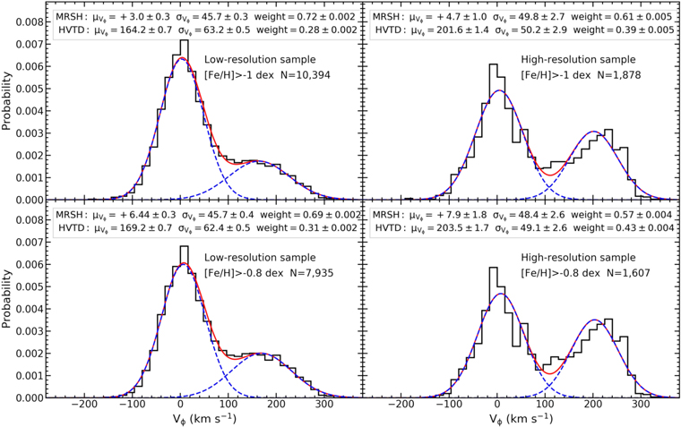
Figure 4. The rotational velocity distribution of the high-velocity sample stars of [Fe/H] > −1.0 dex (top panels) and [Fe/H] > −0.8 dex (bottom panels). The left and right panels are the low-resolution and high-resolution sample stars, respectively. The distribution functions of the rotational velocity are well fitted with a two-Gaussian model according to the lowest BIC. The two single-Gaussian components are interpreted as the metal-rich stellar halo (MRSH) and the high-velocity thick disk (HVTD), and their sum is illustrated by the red curve. The best-fit values of the means (μ), standard deviations (σ), and weights of each single-Gaussian component are given in the corresponding panels, and N represents the number of stars.
Download figure:
Standard image High-resolution imageHere, we use low- and high-resolution samples to confirm each other. It needs to be noted that the fitted parameters from two samples are slightly different, such as the best-fit mean rotational velocity, which is for the low-resolution sample in the top-left panel of Figure 4, while for the high-resolution sample in the top-right panel. But we notice that the two samples show a consistent component number, which implies that the component number does not depend on the sample. In order to be consistent with the type of high-resolution sample stars, we also restrict the effective temperature to K and the surface gravity to log g dex for the low-resolution sample. We find that the fitted parameters from this restricted low-resolution sample are still slightly different from the high-resolution sample, but the difference between the parameters derived from the high-resolution sample and this restricted low-resolution sample has diminished. So, we consider that the differences in the parameters from the two samples could result from uncertainties of the stellar parameters in the low-resolution sample or incompleteness of the high-resolution sample.


A small number of inner-halo stars with [Fe/H] dex have been reported by some study (e.g., An et al. 2013, 2015; Zuo et al. 2017; Liu et al. 2018; Gu et al. 2019). In order to eliminate the effects of the inner halo, we also inspect the component number for stars with [Fe/H] dex. Our results show that the component number is identical for the stars both [Fe/H] and [Fe/H] dex as shown in the bottom panel of Figure 4, which indicates that the effect of the inner halo on our results is negligible. Table 1 lists the best-fit values of the two single-Gaussian components in Figure 4.


Table 1. The Best-fit Values of the Mean (μ), Standard Deviation (σ), and Weight of Each Rotational Velocity Distribution in Gaussian Form in Different Metallicity Intervals
| [Fe/H] | MRSH | HVTD | ||||
|---|---|---|---|---|---|---|
| ⋯ | μ | σ | Weight | μ | σ | Weight |
| (dex) | () | () | ⋯ | () | () | ⋯ |
| Low-resolution Sample | ||||||
| +3.0 ± 0.3 | 45.7 ± 0.3 | 0.72 ± 0.002 | 164.2 ± 0.7 | 63.2 ± 0.5 | 0.28 ± 0.002 | |
| +6.44 ± 0.3 | 45.7 ± 0.4 | 0.69 ± 0.002 | 169.2 ± 0.7 | 62.4 ± 0.5 | 0.31 ± 0.002 | |
| High-resolution Sample | ||||||
| +4.7 ± 1.0 | 49.8 ± 2.7 | 0.61 ± 0.005 | 201.6 ± 1.4 | 50.2 ± 2.9 | 0.39 ± 0.005 | |
| [Fe/H] | +7.9 ± 1.8 | 48.4 ± 2.6 | 0.57 ± 0.004 | 203.5 ± 1.7 | 49.1 ± 2.6 | 0.43 ± 0.004 |


![$[\mathrm{Fe}/{\rm{H}}]\gt -1$](https://content.cld.iop.org/journals/0004-637X/903/2/131/revision1/apjabbd3dieqn87.gif)
![$[\mathrm{Fe}/{\rm{H}}]\gt -0.8$](https://content.cld.iop.org/journals/0004-637X/903/2/131/revision1/apjabbd3dieqn88.gif)
![$[\mathrm{Fe}/{\rm{H}}]\gt -1$](https://content.cld.iop.org/journals/0004-637X/903/2/131/revision1/apjabbd3dieqn89.gif)

Download table as: ASCIITypeset image
We have confirmed that high-velocity stars of [Fe/H] dex contain two independent components using their rotational velocity distribution. According to previous studies, the mean rotational velocity of the thick disk is within the range of 160–200 , and that of the thin disk is greater than 210 (e.g., Kordopatis et al. 2011; Li et al. 2018). For example, Carollo et al. (2010), Li & Zhao (2017), and Li et al. (2018) reported a mean rotational velocity of for the thick disk, and Kordopatis et al. (2011) measured . The halo stars have a lower mean rotational velocity (e.g., Kafle et al. 2017), for example, Smith et al. (2009) measured for the halo stars, Carollo et al. (2010) reported and for the inner halo and outer halo, and Tian et al. (2019) reported that the local halo progradely rotates with . As shown in Figure 4, for the stars with [Fe/H] , one component peaks at for the high-resolution sample and for the low-resolution sample, which is consistent with the thick disk. So, we consider that this component should be the HVTD, and it has the same rotational velocity and metallicity as the canonical thick disk, but its member stars have the same position as the halo in the Toomre diagram. For the stars with [Fe/H] , another component peaks at for the high-resolution sample and for the low-resolution sample, which is similar to the rotational velocity of the halo. Therefore, we regard this component as an MRSH. It has the same rotational velocity and position as the halo in the Toomre diagram, but it has metallicity of the canonical thick disk. Belokurov et al. (2020) measured the rotational velocity distribution of the metal-rich stars with [Fe/H] and on halo-like orbits (Splash stars), with a peak at 25 and standard deviation of 108 ± 19. They showed that a lot of Splash stars have . Because they did not remove disk stars, their Splash stars may be contaminated by the thin- and thick-disk stars. Because there exists a clear gap between the rotational velocity distribution of the HVTD and MRSH as shown in Figure 4, the HVTD is defined as high-velocity sample stars with [Fe/H] dex and , while the MRSH is high-velocity sample stars with [Fe/H] dex and .


We define canonical halo stars as stars with and [Fe/H] < − 1.0 dex. In order to check whether the canonical halo stars contain HVTD or MRSH stars, we study the rotational velocity distribution of the canonical halo that is fitted with a two-peak Gaussian model according to the lowest BIC as shown in Figure 5. Some previous studies showed that the canonical stellar halo has two components: inner halo and outer halo. Thus, we could regard these two single-Gaussian components as the inner halo and outer halo. This implies that the stars with vtot > 220 and [Fe/H] < −1 dex contain very few HVTD or MRSH stars.


Figure 5. The rotational velocity distribution of canonical halo stars with vtot > 220 and [Fe/H] < −1.0 dex for the low-resolution (left panel) and high-resolution samples (right panel). The distribution functions can be fitted with a two-Gaussian model according to the lowest BIC. The two single-Gaussian components are regarded as the inner halo and outer halo, and their sum is illustrated by the red curve. The best-fit values of the means (μ), standard deviations (σ), and weights of each single-Gaussian component are given in the corresponding panels.

Download figure:
Standard image High-resolution image3.2. Kinematic Properties of The MRSH and HVTD
Figure 6 shows the Toomre diagram, Lindblad diagram (a plot of the integrals of motion representing the total energy, E, and vertical angular momentum, Lz), and distribution of orbit eccentricities for the HVTD, MRSH, thick disk, and canonical halo. Our results indicate that there is a relatively clear separation between the HVTD and MRSH in the Toomre diagram, but there is a small amount mixing in the boundary. This also implies that the HVTD and MRSH could be different populations. In addition, in order to present a clear dynamical relation between the HVTD, MRSH, canonical halo, and thick disk, we compare the thick-disk sample stars from Yan et al. (2019) with the HVTD, MRSH, and canonical halo in Lindblad diagram. As shown in the top-right panel of Figure 6, there is an apparent separation between the canonical halo and thick disk as indicated by the blue dashed line. About 65% of the HVTD stars are clustered with the thick disk in the Lindblad diagram, while the other 35% of the HVTD stars are clustered with the canonical halo stars. Furthermore, the HVTD stars contain 23% of high orbital eccentricity (e > 0.8) stars as shown in the bottom-right panel of Figure 6. After excluding those 35% of HVTD stars that have the same position as the canonical halo in the Lindblad diagram, the orbit eccentricity distribution of the HVTD is basically consistent with the thick disk. These indicate that our HVTD stars could be contaminated by MRSH stars and most HVTD stars share the same dynamical properties as the thick disk. As shown in the bottom-left and -right panels of Figure 6, most MRSH stars are clustered with the canonical halo. The orbit eccentricity distribution of the MRSH is basically consistent with the canonical halo, and most of them have high orbit eccentricity (e > 0.6), which is consistent with previous studies (e.g., Belokurov et al. 2020; Fernández-Alvar et al. 2019; Mackereth et al. 2019b). These imply that the MRSH stars share the same dynamical properties as the canonical halo.

Figure 6. Top-left panel: Toomre diagram of the high-velocity thick disk (HVTD, marked by the red dots) and metal-rich stellar halo (MRSH, marked by the cyan dots) for the high-resolution sample. Top-right and bottom-left panels: the distribution between the total energy and the vertical angular momentum (Lindblad diagram) of the thick disk (marked by the black dots), HVTD (marked by the red dots), MRSH (marked by the cyan dots), and canonical halo stars (marked by the orange dots). The blue dashed line represents the separation of populations. Bottom-right panel: distribution of orbit eccentricity of the HVTD (marked by the red dotted line), MRSH (marked by the cyan line), thick-disk stars (black dashed line), and canonical halo stars (orange line).
Download figure:
Standard image High-resolution imageThe gradient of rotational velocity with metallicity is important for the Galactic disk, which can provide useful clues to its formation and evolution. Many works have confirmed that the thin-disk stars show a negative rotational velocity gradient versus metallicity, and the gradient range from ∼−16 to −24 . The thick-disk stars show a positive gradient from ∼ +30 to + 49 (e.g., Lee et al. 2011; Adibekyan et al. 2013; Recio-Blanco et al. 2014; Guiglion et al. 2015; Jing & Du et al. 2016; Yan et al. 2019). Figure 7 shows the variations of rotational velocity with metallicity for the MRSH, HVTD, and halo stars. Variation trends of the MRSH and HVTD stars can be fitted with linear functions, but their gradients are distinctly different. The HVTD has a steeper gradient than the canonical thick disk, . However, the MRSH shows a relatively flat gradient, , which is less than the canonical thick disk. The distribution of rotational velocity with metallicity for the halo stars is more scattered than that of the MRSH and HVTD stars, but it globally exhibits a relatively flat gradient, . The gradient of the halo is basically equal to that of the MRSH. Belokurov et al. (2020) noticed that some metal-rich stars ([Fe/H] > −0.7) show a distinct difference in the rotation velocity versus metallicity distribution for the thin- and thick-disk stars. The distribution of the rotational velocity with metallicity for these metal-rich stars shows a vertical trend, and these metal-rich stars are referred to as Splash stars by Belokurov et al. (2020). The boundaries of the Splash stars have been marked in Figure 7 by a rectangular box. It can be clearly seen that the Splash stars are located in the MRSH.


![${\rm{\Delta }}{V}_{\phi }/{\rm{\Delta }}[\mathrm{Fe}/{\rm{H}}]=+82.2\pm 1.8$](https://content.cld.iop.org/journals/0004-637X/903/2/131/revision1/apjabbd3dieqn132.gif)

![${\rm{\Delta }}{V}_{\phi }/{\rm{\Delta }}[\mathrm{Fe}/{\rm{H}}]\,=+18.0\pm 3.1$](https://content.cld.iop.org/journals/0004-637X/903/2/131/revision1/apjabbd3dieqn134.gif)

![${\rm{\Delta }}{V}_{\phi }/{\rm{\Delta }}[\mathrm{Fe}/{\rm{H}}]=+22.2\pm 1.7$](https://content.cld.iop.org/journals/0004-637X/903/2/131/revision1/apjabbd3dieqn136.gif)


Figure 7. Variation of rotational velocity with metallicity for the MRSH (marked by the cyan dots), HVTD (marked by the orange dots), and halo stars (marked by the yellow-green dots) from our high-resolution sample. These variation trends can be fitted with linear functions using the least-squares method. Stars in the gray rectangle box represent the Splash stars defined by Belokurov et al. (2020).
Download figure:
Standard image High-resolution imageThe HVTD has a steeper gradient than the canonical thick disk in the rotational velocity versus metallicity distribution plane, and the gradient of the HVTD is about twice as high as that of the canonical thick disk. We noticed that the gradient of the rotational velocity versus metallicity in the thick disk depends strongly on the spatial velocity. Figure 8 displays the variation of rotational velocity with metallicity in different spatial velocity intervals for the canonical thick disk from Yan et al. (2019). We can see that the thick-disk stars with show a very flat gradient, , while the thick-disk stars with have a steeper gradient, . This implies that the gradient of the rotation velocity versus metallicity in the thick disk could increase with the spatial velocity. In the HVTD stars with , the gradient of the rotation velocity versus metallicity is steeper than the canonical thick disk, which implies that HVTD stars could belong to the thick disk.


![${\rm{\Delta }}{V}_{\phi }/{\rm{\Delta }}[\mathrm{Fe}/{\rm{H}}]\,=+6.5\pm 0.9$](https://content.cld.iop.org/journals/0004-637X/903/2/131/revision1/apjabbd3dieqn140.gif)


![${\rm{\Delta }}{V}_{\phi }/{\rm{\Delta }}[\mathrm{Fe}/{\rm{H}}]=+40.6\pm 0.8$](https://content.cld.iop.org/journals/0004-637X/903/2/131/revision1/apjabbd3dieqn144.gif)


Figure 8. The variation of rotational velocity with metallicity for the thick-disk stars of (top panel) and (bottom panel).


Download figure:
Standard image High-resolution image4. The Metallicity Distribution of MRSH and HVTD
We obtained the HVTD or MRSH stars selected by rotational velocity distribution and metallicity. The mean metallicities of the HVTD stars are dex with standard deviations of dex for the low-resolution sample, and dex with standard deviations dex for the high-resolution sample. The mean metallicities of the MRSH stars are dex with standard deviations of dex for the low-resolution sample and dex with standard deviations dex for the high-resolution sample. Therefore, the HVTD stars have higher metallicity than the MRSH on average. The metallicity distributions of both high-velocity sample stars are well fitted with a four-peak Gaussian model according to the lowest BIC in Figure 9. The two single-Gaussian components for the canonical halo stars with [Fe/H] dex could be interpreted as the inner halo and outer halo. The relatively metal-rich stars with [Fe/H] dex also exist as two single-Gaussian components, which could be interpreted as the HVTD and MRSH stars. As shown in Figure 9, the canonical halo contains few HVTD and MRSH.
![$\langle [\mathrm{Fe}/{\rm{H}}]\rangle \,=-0.51\pm 0.002$](https://content.cld.iop.org/journals/0004-637X/903/2/131/revision1/apjabbd3dieqn151.gif)
![${\sigma }_{[\mathrm{Fe}/{\rm{H}}]}\,=0.26$](https://content.cld.iop.org/journals/0004-637X/903/2/131/revision1/apjabbd3dieqn152.gif)
![$\langle [\mathrm{Fe}/{\rm{H}}]\rangle =-0.31\pm 0.0004$](https://content.cld.iop.org/journals/0004-637X/903/2/131/revision1/apjabbd3dieqn153.gif)
![${\sigma }_{[\mathrm{Fe}/{\rm{H}}]}=0.31$](https://content.cld.iop.org/journals/0004-637X/903/2/131/revision1/apjabbd3dieqn154.gif)
![$\langle [\mathrm{Fe}/{\rm{H}}]\rangle \,=-0.67\pm 0.001$](https://content.cld.iop.org/journals/0004-637X/903/2/131/revision1/apjabbd3dieqn155.gif)
![${\sigma }_{[\mathrm{Fe}/{\rm{H}}]}=0.20$](https://content.cld.iop.org/journals/0004-637X/903/2/131/revision1/apjabbd3dieqn156.gif)
![$\langle [\mathrm{Fe}/{\rm{H}}]\rangle =-0.60\,\pm 0.0003$](https://content.cld.iop.org/journals/0004-637X/903/2/131/revision1/apjabbd3dieqn157.gif)
![${\sigma }_{[\mathrm{Fe}/{\rm{H}}]}=0.23$](https://content.cld.iop.org/journals/0004-637X/903/2/131/revision1/apjabbd3dieqn158.gif)


Figure 9. Metallicity distribution of the high-velocity stars for the low-resolution (top panel) and high-resolution samples (bottom panel). The distribution functions are well fitted with a four-Gaussian model according to the lowest BIC, which represents the contribution from the outer halo, inner halo, MRSH, and HVTD, and the sum is illustrated by the red curve. The best-fit values of the means (μ), standard deviations (σ), and weights for each single-Gaussian component are given in the corresponding panels.
Download figure:
Standard image High-resolution imageWe noticed that the parameters fitted by the low-resolution and high-resolution samples are slightly different. But two samples show a consistent component number, which implies that the component number does not depend on the sample. In addition, we restrict the effective temperature to K and surface gravity to log g dex for the low-resolution sample in order to be consistent with the high-resolution sample stars. We find that the parameters fitted by this restricted low-resolution sample are still slightly different from the high-resolution sample, but the difference has diminished. So, the parameter differences from the two samples could result from the metallicity uncertainty of the low-resolution sample.


Thus, we have also confirmed the existence of HVTD and MRSH using the metallicity distribution. We now study the variation of the MDFs with vertical distance for these high-velocity sample stars. Figure 10 shows the lowest BIC fitting from the data: a four-peak and a three-peak Gaussian model in the low- and high-resolution samples of and , respectively. The top panel of Figure 10 shows that there are four components within : outer halo, inner halo, MRSH, and HVTD. The inner halo and MRSH occupy the vast majority, and the outer-halo component still exists within . The bottom panel of Figure 10 shows that there are three components in : outer halo, inner halo, and MRSH. The inner halo and MRSH still occupy the majority, but their weights are higher than that of . The weight of the outer-halo component is basically invariable, which implies that the vertical height has little effect on the outer-halo component within . Furthermore, when , the HVTD component disappeared, which indicates that most of the HVTD stars are within . Therefore, the variation of the component weight with vertical height also indicates that MRSH stars belong to the halo, and HVTD stars are attributed to the thick disk. Table 2 lists the best-fit values of the four or three single-Gaussian components in Figures 9 and 10. Belokurov et al. (2020) used K giants identified in the Sloan Digital Sky Survey spectroscopy to show that the Splash population extends as far as , and the ranking of the vertical sizes of the Splash, the disk, and the halo, i.e., , which are consistent with the result of our MRSH.


Figure 10. Metallicity distribution of the high-velocity sample stars for the low-resolution (left panel) and high-resolution sample (bottom panel) in different vertical height intervals. The distribution functions are well fitted with a four-Gaussian or three-Gaussian model according to the lowest BIC. The best-fit values of the means (μ), standard deviations (σ), and weights for each single-Gaussian component are given in the corresponding panels.
Download figure:
Standard image High-resolution imageTable 2. The Best-fit Values of the Mean (μ), Standard Deviation (σ), and Weight (W) of Each Metallicity Distribution in Gaussian Form in Different Vertical Height Intervals
| Outer Halo | Inner Halo | MRSH | HVTD | |
|---|---|---|---|---|
| Low-resolution Sample, kpc | ||||
| μ | −1.69 ± 0.009 | −1.21 ± 0.005 | −0.65 ± 0.003 | −0.56 ± 0.02 |
| σ | 0.29 ± 0.003 | 0.20 ± 0.002 | 0.17 ± 0.002 | 0.39 ± 0.006 |
| W | 0.12 ± 0.003 | 0.30 ± 0.005 | 0.43 ± 0.005 | 0.15 ± 0.009 |
| High-resolution Sample, kpc | ||||
| μ | −2.0 ± 0.007 | −1.34 ± 0.003 | −0.59 ± 0.002 | −0.25 ± 0.002 |
| σ | 0.30 ± 0.004 | 0.23 ± 0.002 | 0.21 ± 0.001 | 0.34 ± 0.006 |
| W | 0.13 ± 0.002 | 0.33 ± 0.003 | 0.37 ± 0.016 | 0.17 ± 0.01 |
| Low Resolution Sample kpc | ||||
| μ | −1.65 ± 0.01 | −1.20 ± 0.006 | −0.65 ± 0.003 | −0.53 ± 0.019 |
| σ | 0.30 ± 0.004 | 0.20 ± 0.002 | 0.17 ± 0.002 | 0.38 ± 0.006 |
| W | 0.12 ± 0.004 | 0.30 ± 0.004 | 0.44 ± 0.005 | 0.14 ± 0.009 |
| High-resolution Sample, kpc | ||||
| μ | −1.96 ± 0.006 | −1.33 ± 0.003 | −0.58 ± 0.005 | −0.14 ± 0.02 |
| σ | 0.29 ± 0.003 | 0.21 ± 0.007 | 0.21 ± 0.003 | 0.27 ± 0.008 |
| W | 0.13 ± 0.002 | 0.27 ± 0.003 | 0.42 ± 0.011 | 0.18 ± 0.012 |
| Low-resolution Sample, kpc | ||||
| μ | −1.80 ± 0.02 | −1.28 ± 0.01 | −0.69 ± 0.01 | ⋯ |
| σ | 0.27 ± 0.007 | 0.20 ± 0.009 | 0.25 ± 0.005 | ⋯ |
| W | 0.17 ± 0.007 | 0.31 ± 0.012 | 0.52 ± 0.015 | ⋯ |
| High-resolution Sample, kpc | ||||
| μ | −2.17 ± 0.016 | −1.41 ± 0.005 | −0.65 ± 0.002 | ⋯ |
| σ | 0.23 ± 0.01 | 0.24 ± 0.003 | 0.29 ± 0.002 | ⋯ |
| W | 0.12 ± 0.005 | 0.42 ± 0.004 | 0.46 ± 0.002 | ⋯ |


Download table as: ASCIITypeset image
The existence of a metal-weak thick disk (MWTD) has been confirmed by several works, such as Morrison et al. (1990), Beers & Sommerlarsen (1995), Chiba & Beers (2000), and Beers et al. (2002, 2014). The MWTD has disk-like kinematics (e.g., Chiba & Beers 2000; Carollo et al. 2010) and is a low-metallicity tail of the thick disk (e.g., Morrison et al. 1990; Beers et al. 2014; Yan et al. 2019). Ivezić et al. (2008) and Carollo et al. (2010) tried to prove the MWTD as an independent stellar population from the thick disk and revealed that its mean rotational velocity could be in the range of 100–150 , while its metallicity values span from −0.8 dex to −1.7 dex. Kordopatis et al. (2013) reported that its lowest metallicity at least goes down to [M/H] dex. Recently, Carollo et al. (2019) reported that the MWTD contains two-times less metal content than the canonical thick disk and exhibits the enrichment of light elements typical of the oldest stellar populations of the Galaxy, and its rotational velocity is ∼150 , with a velocity dispersion of 60 . These properties of the MWTD, including its velocity components and metallicity range, are different from the HVTD and MRSH. Therefore, we consider that HVTD and MRSH could be two different stellar populations from the MWTD.


5. Discussion on the Potential Origins of the MRSH and HVTD
Some previous works have suggested that the metal-rich stars with thick-disk metallicity on halo-like orbits have likely been born in situ rather than having been accreted from satellite systems (e.g., Bonaca et al. 2017; Di Matteo et al. 2018; Haywood et al. 2018; Belokurov et al. 2020; Gallart et al. 2019). Bonaca et al. (2017) kinematically identified halo stars in the solar neighborhood with relative speeds larger than 220 with respect to the local standard of rest based on the RAVE and APOGEE spectroscopic surveys. Because the orbital directions of the metal-rich stars with [Fe/H] are preferentially aligned with the disk rotation, they proposed that these metal-rich halo stars may have formed in situ, rather than having been accreted from satellite systems, and these metal-rich halo stars have likely undergone substantial radial migration or heating. In addition, as part of the metal-rich halo stars, the Splash stars have chemical and kinematic properties similar to our MRSH stars. Because the Splash stars are predominantly old, but not so old as the stars deposited into the Milky Way in the last major merger, Belokurov et al. (2020) concluded that the Splash stars may have been born in the Milky Way's protodisk prior to the massive ancient accretion event that drastically altered their orbits, and they put constraints of the epoch of the last massive accretion event to have finished 9.5 Gyr ago. This massive ancient merger event is Gaia–Sausage (Belokurov et al. 2018; Myeong et al. 2018; sometimes also referred to as Gaia–Enceladus, Helmi et al. 2018). Therefore, according to chemical and kinematic properties, it implies that MRSH stars were born in situ and HVTD stars are part of the thick disk.


On the other hand, the stellar ages are also an effective way to probe the potential origins of the population. However, it is difficult to obtain accurate stellar ages, and different methods of estimating age have systematic differences (Frankel et al. 2019). In this work, we only use the age range of the stars to discuss the potential origins of the MRSH and HVTD. Because the Gaia–Sausage merger could have happened ago (e.g., Belokurov et al. 2018, 2020; Di Matteo et al. 2018; Helmi et al. 2018), we define old stars as older than 9 Gyr and young stars as younger than 9 Gyr. The ages of our sample stars are obtained by cross-matching with two catalogs, the Sanders18 catalog (Sanders & Das 2018) and Wu19 catalog (Wu et al. 2019). Sanders & Das (2018) presented a catalog of stellar distances, masses, and ages for ∼3 million giant stars. The mass and ages have been estimated using the method outlined in Das & Sanders (2019). Sanders & Das (2018) only estimated masses and ages for the stars metal-richer than −1.5 dex, and the maximum age isochrone considered is 12.6 Gyr. Wu et al. (2019) presented a catalog of stellar age and mass estimates for red giant branch (RGB) stars from LAMOST DR4. The estimated age has a median error of 30% for the stars of S/N . The age distributions of the MRSH and HVTD stars are shown in Figure 11. Although the age distributions of the MRSH and HVTD stars inferred from different samples and methods have some differences, these age distributions confirm that both MRSH and HVTD stars contain a certain number of young stars ( Gyr) and old stars ( Gyr).


Figure 11. Age distributions of the MRSH, HVTD, and halo stars. The ages of the stars in the left (middle) panel is obtained by cross-matching between our high-resolution (low-resolution) sample and the Sanders & Das (2018) catalog. The ages of stars in the right panel are obtained by cross-matching between our low-resolution sample and the Wu et al. (2019) catalog. N represents the number of stars. The black dashed lines represent the epoch of the massive merger event (Gaia–Sausage).
Download figure:
Standard image High-resolution imageFor the young stars ( Gyr), their formation may not be affected by the Gaia–Sausage merger. In this regard, the MRSH stars were likely born in situ rather than accreted from the Gaia–Sausage merger. The in situ population can contain stars formed in the initial gas collapse (Samland & Gerhard 2003) and/or stars formed in the disk, which have subsequently been kicked out and placed in the halo (Zolotov et al. 2009; Purcell et al. 2010). However, it is difficult to distinguish between the MRSH stars formed by the initial gas collapse and being heated from the disk. Cooper et al. (2015) listed two different channels of the initial gas collapse to form the in situ stellar halo: stars formed from gas smoothly accreted on to the halo and stars formed in streams of gas stripped from infalling satellites. The "phase wrapping" signature in the disk (e.g., Fux 2001; Minchev et al. 2009; Gómez et al. 2012; de la Vega et al. 2015) and some substructures in the phase space, such as the Gaia snail and spiral (Antoja et al. 2018), are now widely considered to be a relic of a recent external perturbation by a satellite or dwarf galaxy flyby such as Sagittarius (e.g., Antoja et al. 2018; Binney & Schönrich 2018; Bland-Hawthorn et al. 2019; Laporte et al. 2019). In particular, the last pericenter of the orbit of Sagittarius has been shown to have a strong effect on the disk stars (Purcell et al. 2010; Gómez et al. 2012; de la Vega et al. 2015). These external perturbations may heat up disk stars (Mackereth et al. 2019a) and, subsequently, alter their orbits. In addition, the radial migration may also explain the origins of MRSH stars. El-Badry et al. (2016) reported that stars in low-mass galaxies experience significant radial migration via two related processes. First, inflowing and outflowing gas clouds driven by stellar feedback can remain star-forming, and initial orbits of producing stars can be eccentric and have large anisotropy. Second, outflowing and inflowing gas drive strong fluctuations in the overall galactic potential, and stellar orbits are affected by such fluctuations, ultimately becoming heated. Bonaca et al. (2017) concluded that this radial migration mechanism could explain the origin of metal-rich stars on halo-like orbits in the solar neighborhood.

For the old stars formed in situ ( Gyr), the Gaia–Sausage merger event may have a major effect on their formation. The MRSH stars may form in an old protodisk, possibly dynamically heated by the Gaia–Sausage merger, and subsequently be kicked out to the halo. This result is consistent with previous studies (e.g., Di Matteo et al. 2018; Haywood et al. 2018; Belokurov et al. 2020; Gallart et al. 2019). The HVTD stars also form in an old protodisk, but these stars may be much less affected by the Gaia–Sausage merger event than MRSH that they retain some properties of the thick disk.

6. Summary and Conclusions
Based on a high-resolution sample of G-/K-type giant stars from the APOGEE DR14 and a low-resolution sample of A-, F-, G-, and K-type stars from the LAMOST spectroscopic survey combined with the Gaia DR2 survey, we obtained high-velocity sample stars ( ) in the Toomre diagram. From the kinematic and chemical distribution of these high-velocity sample stars, we concluded that MRSH and HVTD exist in the Galaxy, and studied their kinematic and chemical properties.


The rotational velocity distribution of sample stars with and [Fe/H] dex can be well described by a two-Gaussian model, associated with the HVTD and MRSH. We also confirmed that the metallicity distribution of the sample stars can be described by a four-Gaussian model: outer halo, inner halo, MRSH, and HVTD. The HVTD has basically the same rotational velocity and metallicity as the canonical thick disk, and it shares the same dynamical properties as the thick disk. However, their member stars have the same position as the halo in the Toomre diagram. The MRSH shows basically the same rotational velocity, orbit eccentricity, and position in the Lindblad and Toomre diagrams as the canonical halo, but their metallicity distribution is similar to that of the thick disk.


In addition, we found that the outer-halo component still exists within , and the increase of vertical height has little effect on the proportions of the outer-halo component in . Among these stars with , , and , the inner halo and MRSH occupy the vast majority, and most of the HVTD stars are within , and they have higher metallicity than MRSH stars on average, and the canonical halo contains very few HVTD or MRSH stars. For the HVTD, there exists a steeper gradient of rotational velocity with metallicity than the canonical thick disk. However, the gradient of the rotational velocity with metallicity for the MRSH is flatter than that of the canonical thick disk. Their chemical and kinematic properties and age imply that the MRSH and HVTD stars may form in situ rather than being accreted from satellite systems.


We especially thank the referee for insightful comments and suggestions, which have improved the paper significantly. This work was supported by the National Natural Foundation of China (NSFC No. 11973042 and No. 11973052). This project was developed in part at the 2016 NYC Gaia Sprint, hosted by the Center for Computational Astrophysics at the Simons Foundation in New York City. The Guoshoujing Telescope (the Large Sky Area Multi-Object Fiber Spectroscopic Telescope, LAMOST) is a National Major Scientific Project built by the Chinese Academy of Sciences. Funding for the project has been provided by the National Development and Reform Commission. LAMOST is operated and managed by the National Astronomical Observatories, Chinese Academy of Sciences.
Funding for the Sloan Digital Sky Survey IV has been provided by the Alfred P. Sloan Foundation, the US Department of Energy Office of Science, and the Participating Institutions. SDSS-IV acknowledges support and resources from the Center for High-Performance Computing at the University of Utah. The SDSS website is www.sdss.org.
SDSS-IV is managed by the Astrophysical Research Consortium for the Participating Institutions of the SDSS Collaboration including the Brazilian Participation Group, the Carnegie Institution for Science, Carnegie Mellon University, the Chilean Participation Group, the French Participation Group, Harvard-Smithsonian Center for Astrophysics, Instituto de Astrofísica de Canarias, Johns Hopkins University, Kavli Institute for the Physics and Mathematics of the Universe (IPMU)/University of Tokyo, Lawrence Berkeley National Laboratory, Leibniz Institut für Astrophysik Potsdam (AIP), Max-Planck-Institut für Astronomie (MPIA Heidelberg), Max-Planck-Institut für Astrophysik (MPA Garching), Max-Planck-Institut für Extraterrestrische Physik (MPE), National Astronomical Observatories of China, New Mexico State University, New York University, University of Notre Dame, Observatário Nacional/MCTI, The Ohio State University, Pennsylvania State University, Shanghai Astronomical Observatory, United Kingdom Participation Group, Universidad Nacional Autónoma de México, University of Arizona, University of Colorado Boulder, University of Oxford, University of Portsmouth, University of Utah, University of Virginia, University of Washington, University of Wisconsin, Vanderbilt University, and Yale University.
This work has made use of data from the European Space Agency (ESA) mission Gaia (http://www.cosmos.esa.int/gaia), processed by the Gaia Data Processing and Analysis Consortium (DPAC, http://www.cosmos.esa.int/web/gaia/dpac/consortium). Funding for DPAC has been provided by national institutions, in particular the institutions participating in the Gaia Multilateral Agreement.
Appendix A: Distance and Velocity Estimation
We determined the distance and velocity for more than 300,000 giant stars from the LSS-GAC DR4 and Gaia DR2 catalog (Yan et al. 2019). Here, we use the Bayesian approach to estimate the distance and velocity of the sample stars with (Bailer-Jones 2015; Astraatmadja & Bailer-Jones 2016a, 2016b; Bailer-Jones et al. 2018; Luri et al. 2018) and compare the results with other works.

Our goal is to obtain the posterior probability of observed stars, and the posterior can be written as


where data vector , ϖ denotes stellar parallax, and are proper motion in R.A. and decl., respectively, and the symbol "T" represents the matrix transpose. The parameters vector is written as , consisting of the heliocentric distance (d), tangential speed (v), and travel direction (ϕ, increasing counterclockwise from north). , where . is a covariance matrix:


where denotes the correlation coefficient between the astrometric parameters i and j. is the error of the astrometric parameters k. represents the prior distribution of the parameters vector, (Luri et al. 2018), here


We use the exponentially decreasing space density prior for distance (Bailer-Jones 2015; Bailer-Jones et al. 2018) and adopt the Galactic-longitude- and -latitude-dependent length scale (Bailer-Jones et al. 2018), , which is obtained by fitting a spherical harmonic model. We assume that the prior over the angle ϕ is uniform. The prior over speed is a beta distribution, and we adopt , , and .


The posterior probability of observed stars can be obtained by using the Equations (A1). We use the Markov Chain Monte Carlo (MCMC) sampler EMCEE (Goodman & Weare 2010; Foreman-Mackey et al. 2013) to characterize the posterior probability. For each star, we run each chain using 100 walkers and 100 steps, for a total of 10,000 random samples drawn from the posterior distribution. Because the radial velocity does not depend on parallax and proper motion, we also sample 10,000 random samples for radial velocity and assume uniform priors on radial velocity. Therefore, for each star, we obtained 10,000 posterior samples including its heliocentric distance (d), tangential speed (v), direction of travel (ϕ), and radial velocity (rv). These random samples are used to derive the Cartesian Galactocentric coordinate (), the projected distance from the Galactic center, Galactic velocity components , and Galactocentric cylindrical component as described in Section 2.2. The median is used as an estimator of these astrophysical quantities, and the standard deviation of the quantities is used to define the uncertainty in the estimated value.


Bailer-Jones (2015) discussed in detail how the distance derivation by inverting the parallax is not appropriate when the relative parallax error is above 20%. So, we also compare distances of our sample stars with the Sanders18 catalog (Sanders & Das 2018). We cross-match between LAMOST DR5, Gaia DR2, and the BailerJones18 catalog. Bailer-Jones et al. (2018) inferred distances for all 1.33 billion stars with parallaxes in Gaia DR2 using a weak distance prior distribution that varies smoothly as a function of Galactic longitude and latitude according to a Galaxy model. Panel (a) of Figure A1 shows that the distances of stars with a relative error in parallax can be determined precisely just by inverting the parallax. As shown in panel (b) of Figure A1, for the stars with , estimating distances by inverting the parallax may lead to deviation when the distance to the stars is above 2 kpc. Panel (c) of Figure A1 compares distance estimates obtained by Bayesian inference with the Sanders18 catalog. We notice that the Bayesian inference performs better than inverting the parallax for stars with . Therefore, in this work, we choose different methods for deriving the distance for stars with and .


Figure A1. Comparisons of the distance estimation of our sample stars with Bailer-Jones et al. (2018, dBailer). The stars in panel (a) have a relative error in parallax . Their distances () are obtained by inverting the parallax. The stars in panels (b) and (c) have a relative error in parallax f > 0.1. The distances of the former (dInversion) are calculated by inverting the parallax, while the distances of the latter (dBayesian) are determined using Bayesian analysis. The black solid line represents the 1:1 line. N represents the number of subsample stars.


Download figure:
Standard image High-resolution imageWe also compare our distances and velocities with other works such as the BailerJones18 catalog (Bailer-Jones et al. 2018) and the Sanders18 catalog (Sanders & Das 2018) in Figure A2. Panel (a) of Figure A2 compares the distance estimates from Bailer-Jones et al. (2018, ) and this work (). From this panel, we see that the distances of our sample stars are very well consistent with the results in Bailer-Jones et al. (2018), 93% of stars have , of stars have , and of stars have (only few stars with ). Sanders & Das (2018) also presented a catalog of stellar distances, masses, and ages for ∼3 million giant stars from large spectroscopic surveys (including APOGEE DR14). We also cross-match between APOGEE DR14, Gaia DR2, and the Sanders18 catalog (i.e., our initial high-resolution sample), for a total of 155,355 stars. We compare the radial distance, vertical height, and rotational velocity of these stars with those in the Sanders18 catalog in panels (b)–(d) of Figure A2, and our distance and velocity estimates are basically consistent with the results in Sanders & Das (2018). These imply that our comparison does not show significant bias.


Figure A2. Distance and velocity estimation comparisons. Panel (a) compares the distance of this work with the BailerJones18 catalog (Bailer-Jones et al. 2018). Panels (b)–(d) compare the radial distance, vertical height, and rotational velocity in Galactocentric cylindrical coordinates with the Sanders18 catalog (Sanders & Das 2018). The color bar represents the number of stars. The black solid line represents the 1:1 line.
Download figure:
Standard image High-resolution imageAppendix B: Comparison of Stellar Parameters
In this work, we have 695 stars in common the between high-resolution and low-resolution samples, and the comparisons of metallicity, effective temperature, and surface gravity for these common stars are given in Figure B1. We also commented on the similarities and differences of the MDFs based on the two samples. In order to validate the LAMOST stellar parameters, there are several independent works comparing the parameters of LAMOST with other reliable databases (including APOGEE; e.g., Wu et al. 2011; Guo Yan-Xin et al. 2015; Luo et al. 2015; Xiang et al. 2015). For example, Luo et al. (2015) compared the parameters of the LAMOST with those of the APOGEE, and these parameters include radial velocity, effective temperature, surface gravity, and metallicity. These comparisons do not show significant statistical deviations. For example, the mean difference of the metallicity between the LAMOST and the APOGEE is −0.09 dex, and the standard deviation is 0.08 dex. The mean difference of the effective temperature between the LAMOST and the APOGEE is 1 K, and the standard deviation is 76 K. The mean difference of the surface gravity is 0.08 dex, and the standard deviation is 0.28 dex. As shown in Figure B1, our comparison does not show significant bias, which is basically consistent with the results of Luo et al. (2015). Although there are a small number of low-resolution stars that their parameters (e.g., surface gravity) deviate slightly from those of high-resolution stars in Figure B1, the influence of a single star could be ignored when the number of sample stars is large enough.

Figure B1. A comparison of metallicity ([Fe/H]), effective temperature (Teff), and surface gravity (log g) for the stars in common between the low-resolution and high-resolution samples. In panel (a), and represent the metallicity of the low-resolution and the high-resolution stars, respectively. Δ[Fe/H] represent − . μ and σ stand for the mean and standard deviation of Δ[Fe/H], respectively. The symbols in panels (b) and (c) are also similar.
![${[\mathrm{Fe}/{\rm{H}}]}_{\mathrm{LAMOST}}$](https://content.cld.iop.org/journals/0004-637X/903/2/131/revision1/apjabbd3dieqn240.gif)
![${[\mathrm{Fe}/{\rm{H}}]}_{\mathrm{APOGEE}}$](https://content.cld.iop.org/journals/0004-637X/903/2/131/revision1/apjabbd3dieqn241.gif)
![${[\mathrm{Fe}/{\rm{H}}]}_{\mathrm{LAMOST}}$](https://content.cld.iop.org/journals/0004-637X/903/2/131/revision1/apjabbd3dieqn242.gif)
![${[\mathrm{Fe}/{\rm{H}}]}_{\mathrm{APOGEE}}$](https://content.cld.iop.org/journals/0004-637X/903/2/131/revision1/apjabbd3dieqn243.gif)
Download figure:
Standard image High-resolution imageIt needs to be noted that the horizontal branch does not seem distinct for the low-resolution sample in the bottom panel of Figure 2. In order to check whether the accuracy of the parameters' effects on it, we also restrict the error of the effective temperature to smaller than 70 K, the error of the surface gravity to smaller than 0.1 dex, and the S/N to in the g band for the low-resolution sample. However, the horizontal branch does not still seem to be very distinct. So, we consider that it could be due to sample selection in the LAMOST survey. In addition, we only use the metallicity and radial velocity of the LAMOST sample in this study; the accuracy of temperature and surface gravity would not affect our final results.
