


Abstract
We use K-giant stars selected from the LAMOST DR5 to study the variation of the rotational velocity of the Galactic halo at different space positions. Modeling the rotational velocity distribution with both the halo and disk components, we find that the rotational velocity of the halo population decreases almost linearly with increasing vertical distance to the Galactic disk plane, Z, at fixed galactocentric radius, R. The samples are separated into two parts with and . We derive that the decreasing rates along Z for the two subsamples are −3.07 ± 0.63 and −1.89 ± 0.37 km s−1 kpc−1, respectively. Comparing with the TNG simulations, we suggest that this trend is caused by the interaction between the disk and halo. The results from the simulations show that only an oblate halo can provide a decreasing rotational velocity with increasing Z. This indicates that the Galactic halo is oblate with galactocentric radius . On the other hand, the flaring of the disk component (mainly the thick disk) is clearly traced by this study; with R between 12 and 20 kpc, the disk can vertically extend to above the disk plane. What is more interesting is that we find the Gaia–Enceladus–Sausage component has a significant contribution only in the halo with , i.e., a fraction of 23%–47%, while in the outer subsample, the contribution is too low to be well constrained.


1. Introduction
The stellar halo is one of the most important components in the Milky Way. Under the paradigm of the Λ cold dark matter model, the halo is formed through accretion and merging of satellites, and plenty of substructures are considered to be retained therein. So the halo has been recording information about its formation history. As a result, studies of the stellar halo can directly help us understand the formation of the Milky Way. However, the stellar halo is the most difficult component to study. It is relatively diffuse and of low density, and it can reach out to distances over 100 kpc (Bland-Hawthorn & Gerhard 2016). That makes it hard to obtain velocity information, i.e., proper motions and radial velocities. What is more, distance is also difficult to accurately determine, except for standard candles like RR Lyrae stars or blue horizontal branch stars (Xue et al. 2008; Hernitschek et al. 2018; Thomas et al. 2018). Thus the main obstacle to studying the properties of the stellar halo is obtaining a sufficient sample of tracers.
Thanks to the rapid development of large survey projects, e.g., the Sloan Digital Sky Survey (York et al. 2000), the Panoramic Survey Telescope and Rapid Response System (Bernard et al. 2016) and the Gaia mission (Gaia Collaboration et al. 2016, 2018a), many of those embedded substructures have been discovered in the halo, e.g., the Sagittarius Stream (Ibata et al. 1994), the GD-1 Stream (Grillmair & Dionatos 2006a, 2006b), and the ω-Cen Stream (Ibata et al. 2019). Those substructures, especially the thin cold streams, are helpful for studying the halo profile. Lux et al. (2013) introduced a method using the Markov chain Monte Carlo technique to constrain the halo shape with thin streams. The streams NGC 5466 and Pal 5 proved to be the best candidates from their orbit properties. Sanderson et al. (2015) studied how to constrain the halo profile with action distributions of streams. The results showed that, even for the simple case of a spherical potential, at least 20 streams with more than 100 member stars are required to ensure the potential is well constrained. Law & Majewski (2010) introduced a triaxial model which successfully reproduced the most prominent stream, the Sagittarius Stream. But there are still some points that are inconsistent with subsequent observations (see Dierickx & Loeb 2017 and references therein). Vera-Ciro and Helmi (2013) studied the halo shape using the Sagittarius Stream taking into account the effect of the Magellanic Clouds; their results suggested an oblate halo. From all of these studies, we find that the streams are powerful tracers to constrain the halo profile.
Many direct efforts, other than using tidal substructures, have also attempted to profile the halo. Valluri et al. (2012) showed that the halo shape can be probed using the orbital properties of individual halo stars, e.g., the action and frequency. Results from complementary simulations show that the disk plays an important role in the shape of the inner halo, making it oblate, but not the outer part. Using K-giant stars selected from data release 5 (DR5) of the Guoshoujing Telescope (Large Sky Area Multi-Object Fiber Spectroscopic Telescope; LAMOST), Xu et al. (2018) demonstrated a complicated halo, the profile being different for the inner and outer parts. Traced by the K-giant stars selected from the LAMOST DR5, the shape of the halo varies from oblate for the inner part to almost spherical for the outer part.
To determine the interaction between different components of the Milky Way, we require a deep analysis of their dynamics. The second data release of the Gaia mission (Gaia DR2) contains proper motions and parallaxes for more than 1.3 billion stars, and radial velocities for stars brighter than 14 in the G-band (Gaia Collaboration et al. 2018a). Accurate astrometric data greatly improve the study of the dynamics of the disk and halo (Belokurov et al. 2020). The phase spiral signature in the local volume was discovered by Gaia Collaboration et al. (2018b) and Antoja et al. (2018) for the first time, which indicates a possible interaction between the satellites of the Milky Way and the disk (Laporte et al. 2019; Y. Xu et al. 2020, in preparation). Spectroscopic surveys, including APOGEE and LAMOST, have made great progress in the study of the Milky Way. The combination of the APOGEE/LAMOST and Gaia data sets provides a unique opportunity to study the formation of the halo. Combining the astrometric data of Gaia DR2 and APOGEE, Helmi et al. (2018) revealed a major merger event in the local volume, named Gaia–Enceladus (also known as Gaia–Sausage; Belokurov et al. 2018). Using the combination of LAMOST and Gaia DR2, Tian et al. (2019, hereafter Paper I) measured a rotational velocity of km s−1 of the halo in the solar neighborhood using the K-giant sample.

According to the studies of Rodriguez-Gomez et al. (2017), the morphology for massive and dwarf galaxies significantly depends on their assembly history and spin, respectively. For Milky Way-like galaxies, the morphology depends on a combination of the two factors. To determine whether the halo shape is related to the spin variance, as in Paper I, we will also use K-giant stars to further study the rotation of the halo. The K-giant stars are perfect tracers for studying the dynamics of the halo; first, giant stars have higher luminosity, which is helpful in tracing distant volumes. Second, the K-giant stars are high in number, providing enough samples for statistics, especially for studies on the global properties of the stellar halo.
The LAMOST is a 4 m, quasi-meridian, reflecting Schmidt telescope. There are 4000 fibers, which make it efficient in obtaining spectra. DR5 provides radial velocities and metallicities for millions of stars with uncertainties of ∼5 km s−1 and 0.1 dex respectively. The high efficiency allows LAMOST to obtain more than nine million spectra, the largest observation sample. Combined with Gaia DR2, it provides an unprecedented opportunity to study the Milky Way. More recently, DR7 includes low- and medium-resolution spectra6 with R = 1800 and 7500, respectively.
This paper is organized as follows. In Section 2, we briefly introduce the data set and the method. The results are shown in Section 3. Discussions are given in Section 4.
2. Data and Method
As in Paper I, we use the K-giant stars selected from LAMOST DR5 (Liu et al. 2014) to study the rotation velocities of the halo and thick disk. The LAMOST DR5 data set provides radial velocity and metallicity, with typical errors of ∼5 km s−1 and 0.1 index, respectively. Following Paper I, we remove all stars with metallicity [Fe/H] to reduce contamination from the disk, especially the thin disk stars (see Figure 4 in Hayden et al. 2015). This proves to be efficient (as shown in Paper I). In this project, we address larger volumes, where the distances of the stars are no longer available from Gaia DR2. We adopt the distances provided by Carlin et al. (2015), which are estimated using a Bayesian approach by comparing the stellar parameters and a grid of stellar isochrones with typical relative errors ∼20%.

To avoid systematic offset of the distances and radial velocities from LAMOST DR5 (Tian et al. 2015; Schönrich & Aumer 2017; and Paper I), we use the common stars of LAMOST DR5 and Gaia DR2 to determine the offset and correct the values from the former. The distance is normalized by 0.805 and the radial velocity is corrected by adding ∼5.38 km s−1. More details on distance and radial velocity corrections are described in Appendices A and B, respectively.
The proper motions of the K-giant star samples are obtained by cross-matching with Gaia DR2, and the positions and velocities are calculated using the Python package Galpy (Bovy 2015). The solar motion relative to the local standard of rest from Schönrich et al. (2010) is adopted: km s−1.

In order to study the variance of the rotational velocity of the halo at different heights to the disk plane, a sufficient sample for each volume is required. We first focus on the volumes with , , and in galactocentric cylindrical coordinates as shown in Figure 1. We adopt the solar location from Reid et al. (2014) with (R, ϕ, Z) = (8.3 kpc, 0°, 0 kpc). Here we ignore the distance from the Sun to the disk plane, which is too small to make any difference to our results. To constrain the uncertainties, only those stars with signal-to-noise ratio higher than 10, radial velocity errors km s−1, and proper motion errors (, ) smaller than 0.3 mas yr−1 are used. This is labeled as the S-sample. A similar sample with different R range, , is selected for studying the outer part, labeled as the SO-sample in Figure 1.


Along the height to the disk plane, we divide each of the two samples into six sub-volumes to ensure each sub-volume contains enough stars. The information for each sub-volume is listed in Table 1.
Table 1. Information for Each Subsample of Stars
| Selection | fH | VϕH | fD | fH3 | N | ||||||
|---|---|---|---|---|---|---|---|---|---|---|---|
| (km s−1) | (km s−1) | (km s−1) | (km s−1) | (km s−1) | (km s−1) | ||||||
| S | −1 < Z < 1 | 0.70 + 0.04−0.04 | 37 + 7−7 | 75 + 4−4 | 0.30 | 185 + 5−5 | 41 + 3−3 | ⋯ | ⋯ | ⋯ | 2215 |
| 1 < Z < 2 | 0.81 + 0.04−0.05 | 50 + 5−6 | 79 + 3−4 | 0.19 | 177 + 5−6 | 38 + 4−4 | ⋯ | ⋯ | ⋯ | 2268 | |
| 2 < Z < 4 | 0.12 | −18 + 41−64 | 82 + 17−16 | 0.41 + 0.06−0.07 | 127 + 9−9 | 55 + 4−4 | 0.47 + 0.09−0.11 | 12 + 4−4 | 33 + 5−7 | 3415 | |
| 4 < Z < 6 | 0.77 + 0.05−0.09 | 40 + 6−4 | 73 + 3−3 | ⋯ | ⋯ | ⋯ | 0.23 | 6 + 7−7 | 18 + 16−12 | 1731 | |
| 6 < Z < 10 | 0.68 + 0.05−0.05 | 24 + 4−4 | 82 + 4−3 | ⋯ | ⋯ | ⋯ | 0.32 | 14 + 4−5 | 12 + 10−8 | 1327 | |
| 10 < Z < 15 | 1 | 10 + 4−4 | 63 + 3−3 | ⋯ | ⋯ | ⋯ | ⋯ | ⋯ | ⋯ | 496 | |
| SO | −1 < Z < 1 | 0.60 + 0.04−0.04 | 23 + 11−10 | 80 + 13−12 | 0.40 | 221 + 2−3 | 20 + 3−3 | ⋯ | ⋯ | ⋯ | 287 |
| 1 < Z < 2 | 0.86 + 0.03−0.04 | 20 + 7−6 | 59 + 10−7 | 0.14 | 201 + 7−10 | 28 + 11−8 | ⋯ | ⋯ | ⋯ | 218 | |
| 2 < Z < 4 | 0.92 + 0.02−0.02 | 20 + 3−3 | 46 + 4−4 | 0.08 | 194 + 8−14 | 32 + 11−6 | ⋯ | ⋯ | ⋯ | 537 | |
| 4 < Z < 6 | 0.95 + 0.01−0.02 | 9 + 4−4 | 54 + 4−4 | 0.05 | 201 + 9−17 | 28 + 16−8 | ⋯ | ⋯ | ⋯ | 482 | |
| 6 < Z < 10 | 0.97 + 0.01−0.01 | 6 + 3−3 | 53 + 3−3 | 0.03 | 192 + 18−26 | 45 + 22−17 | ⋯ | ⋯ | ⋯ | 639 | |
| 10 < Z < 15 | 1 | 1 + 4−4 | 60 + 4−4 | ⋯ | ⋯ | ⋯ | ⋯ | ⋯ | ⋯ | 395 | |


Note. The results, including fraction f, the rotational velocity and dispersions , from the Bayesian method for each component are listed. Symbols H, D, and 3 denote the disk, halo and the third component, respectively. The last column lists the number of the K-giant stars in each sub-sample.


Download table as: ASCIITypeset image
In Paper I, a Bayesian model including three Gaussian components was used for the local volume: the halo, the thick disk, and a possible retrogradely rotating component. In this paper, we adopt the same method and include the halo, the thick disk and a possible additional component. The Gaussian distribution of each component can be written as follows:

where and are the rotational velocity and its dispersion of the ith component, fi is the number fraction of the ith component, and and are the rotational velocity and its uncertainty of the kth star in cylindrical coordinates. Considering that the errors in the rotational velocity will be larger for distant stars, which may affect the results, here we use the probability calculation with uncertainties included, as shown in Equation (1). To determine the rotational velocities of the three components, the Python package emcee is applied to the samples with different space selections as listed in Table 1. An affline solver is used with 50 walkers and 6000 iterations in total, including 3000 burn-in iterations. To find the best-fit parameters for the components, we test models with different numbers of components, e.g., 1, 2, or 3 according to the results given in Paper I. The median values are adopted for each of the parameters. The lower and upper uncertainties are determined from the differences between the median value and the 16% and 84% values. A typical result for the parameter determination is showed in Appendix C. Due to the large contribution from the disk, the third component has a low fraction in the lower volumes; in this paper, we have much fewer stars in each volume than in Paper I.


We find that the model with the disk and halo components is better for volumes with . As the contamination of the disk becomes lower for higher volume, i.e., , the model with the halo and retrogradely rotating components is better, rather than the halo and the disk. In general, the disk contributes very few stars () in those higher-Z volumes (Z = 5 kpc) around R = 9 kpc (Wang et al. 2018). As a result, the contributions of the halo and the additional contribution will rise. In Table 1, for the transition volume with in the S-sample, the disk contribution becomes weaker and the third component (the Gaia–Enceladus–Sausage (GES) as described in the following section) increases. Then we constrain the parameters of a model with all three components. This is not done for the volume with similar height in the SO-sample because of the low number of samples and the low contribution of the GES component (see below). The median values are adopted as the best-fit parameters for each volume. The results for those space volumes are listed in Table 1. The markers H, D, and 3 denote the halo, the disk, and the third component, respectively.


Figure 1. Space distribution of the K-giant sample. The dashed and dotted lines represent the limits on θ and R in a cylindrical frame, and 30° for θ and 6, 12, and 20 kpc for R from inner to outer.

Download figure:
Standard image High-resolution image3. Results
Figure 2 presents the distributions of the rotational velocity and its dispersion.
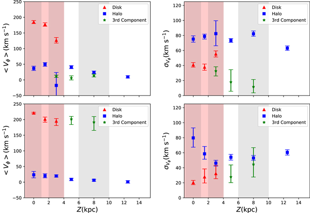
Figure 2. Distributions of the rotation velocity and its dispersion in the left and right panels, respectively. The gray shadowed columns represent the bin range along Z. The red shadowed region represents height lower than 4 kpc, where the disk component is always included in the Bayesian model. The top and bottom panels show the results from the S-sample and SO-sample, respectively. The blue and red symbols represent the parameters of the halo and disk components, respectively. The green symbols show the parameters of the Gaia–Enceladus–Sausage component in the S-sample, or the extension of the disk in the SO-sample. The errorbars represent the uncertainties of the values obtained from Markov chain Monte Carlo simulations.
Download figure:
Standard image High-resolution image3.1. Rotational Velocity Distribution of the Halo
Focusing on the halo component, which is the main target in this paper, we find that the halo in the S-sample (the blue symbols in Figure 2) is progradely rotating with rotational velocity dispersion around 75 km s−1. The rotational velocity generally decreases with height to the disk plane. This is clearer in the left panel in Figure 3. The black solid line shows the linear fitting results, with rotational velocity uncertainties taken into account. The fitting results show that the decreasing rate is −3.04 ± 0.63 km s−1 kpc−1. The intercept of the line represents the rotational velocity of the halo at the disk plane, of 49 ± 5.34 km s−1. The volume with shows an exception of the variance. The uncertainties in the parameters are very large, because the fraction () of the halo is too low to be well constrained.


Figure 3. Rotational velocity distributions of the halo in the S-sample and SO-sample versus height to the disk in the top and bottom panels with the blue symbols, respectively. The solid black lines represent the regression linear relation. The parameters for the regression are given in the top right corner.
Download figure:
Standard image High-resolution imageUnlike in the S-sample, the rotational velocity dispersion is no longer flat in the SO-sample, but first decreases and then remains around a lower value of 60 km s−1. This is consistent with the variance of the rotational velocity dispersion showed by Bird et al. (2019).
Similar to the S-sample, the SO-sample shows a decreasing trend of the rotational velocity of the halo. As shown in the right panel of Figure 3, the decreasing rate of the rotational velocity is lower than that of the S-sample, of −1.89 ± 0.37 km s−1 kpc−1. The intercept of the fitting line is of 22.40 ± 2.66 km s−1. This is much lower than that of the S-sample, meaning the rotational velocity of the halo close to the disk plane is larger for the inner part.
3.2. Contribution of the GES
The locations with show a second halo component with low rotational velocity dispersion and close-to-zero rotational velocity (the green symbols in the top panels). This is consistent with the properties of the GES (Belokurov et al. 2018; Helmi et al. 2018; Myeong et al. 2019). It should be noted that the GES component is not recognized in the lower volumes. That does not mean there is no contribution of the GES component in those volumes; the main reason is that the fraction of the GES member stars is too low to be well constrained at lower-Z locations.

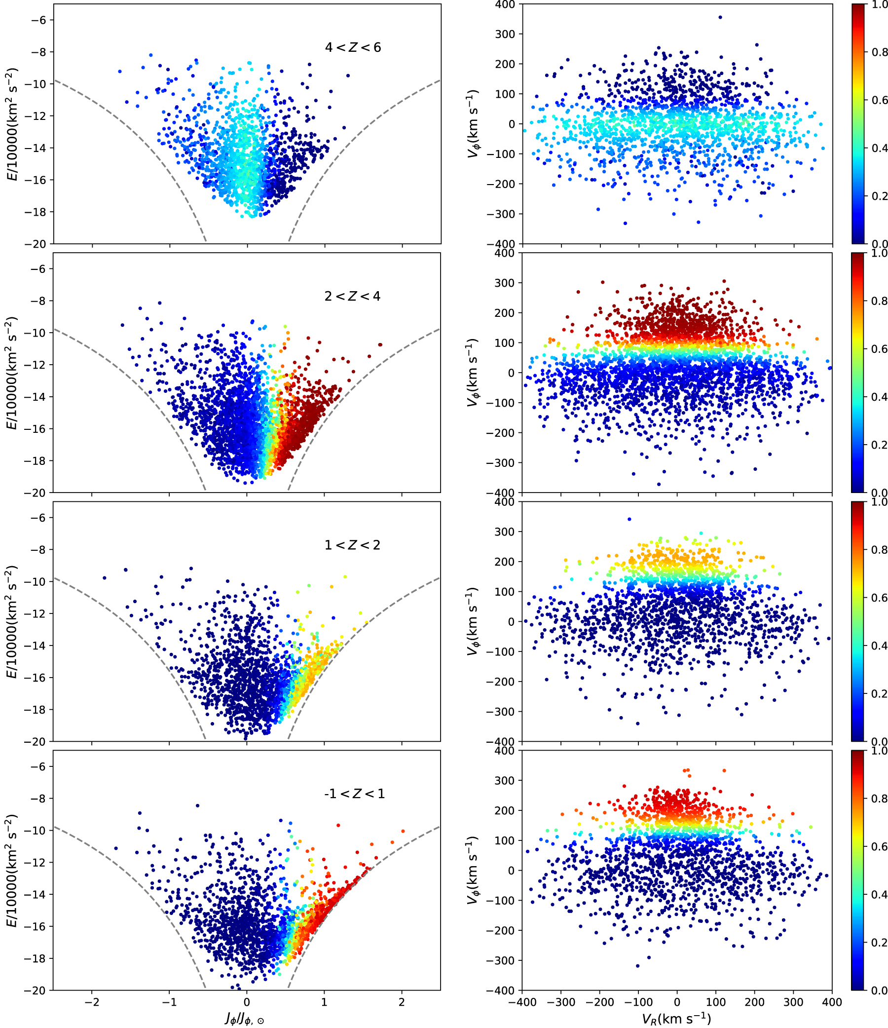
According to the distribution of the components, we calculate the probabilities of the components for each star. Figures 4 and 5 show the distributions of the stars in each volume color-coded by the probability of the disk component. Because the disk component almost vanishes in the higher volumes in the S-sample, where there are only the halo and GES components, we present the probability of the GES in the subsample with (the top left panel in Figure 4).


Figure 4. Phase space distributions of stars in the different volumes from the S-sample. The left and right panels show the distribution in action versus energy E and velocity space, respectively. The stars are color-coded by the probability of belonging to the disk component for the volumes with , or the probability of belonging to the GES component for the volume with . The dashed lines in the left panels represent the circular orbits. From top to bottom, the panels represent volumes with different heights, e.g., , , , −1 < Z < 1 kpc.


Download figure:
Standard image High-resolution image
Figure 5. Similar to Figure 4, but for stars from the SO-sample. From top to bottom, the panels represent volumes with different heights, i.g. 6 < Z < 10 kpc, 4 < Z < 6 kpc, 2 < Z < 4 kpc, 1 < Z < 2 kpc, −1 < Z < 1 kpc. The dots are color-coded by the probability of belonging to the disk component.
Download figure:
Standard image High-resolution imageThe GES is included in the Bayesian model as an independent component, because it has significantly different dynamical information from the halo (Helmi et al. 2018), smaller rotational velocity and dispersion, and larger energy. As shown in Figures 4 and 5, the probabilities for the GES member stars are around 50% at most. That means it is quite difficult to select a pure sample to study its chemical information. In Figure 6, the metallicity distributions of the stars with probability higher or lower than 0.4 in the S-sample with are shown. We find that the distribution with higher probabilities is still different from that of Helmi et al. (2018), because of the high contamination ().


Figure 6. Histogram distribution of metallicity of stars in the S-sample with 4 < Z < 6 kpc. The distributions of stars with probability higher and lower than 0.5 are represented by blue and red symbols, respectively.
Download figure:
Standard image High-resolution imageWhat should be noted is that the GES component is more significant in the top right panel in Figure 4, where the stars are located with , but this is not clear for the outer volumes with in Figure 5. It is not clear that the missing GES is intrinsic or that the larger uncertainties of the distances make the distribution of the action Jϕ more diffuse.


3.3. Rotational Velocity Distribution of The Disk
For the disk component, the variances of the rotational velocity and its dispersion are also obtained with the sample [Fe/H] , even though this may not represent the whole typical thick disk. What should be noted is that our model using the Bayesian method does not include the metal-weak thick disk (Carollo et al. 2019) as a independent component, because of the low fraction in our sample.

From the top panels in Figure 2 which represent the results of the S-sample, we find that the rotational velocity of the disk component (red symbols) decreases with increasing height to the disk plane, while the dispersion increases. As those stars with metallicity [Fe/H] are removed, there are too few thin disk stars left in our sample (Hayden et al. 2015) to give a significant offset. From Table 1, we find that the rotational velocity is around km s−1 for the volume , which also suggests that it is contributed by the thick disk component (Morrison et al. 1990). It decreases to 127 km s−1 of the volume with for the S-sample. Meanwhile, the dispersion of the rotational velocity increases from 41 km s−1 at lowest volume to 55 km s−1. The decreasing trend of the rotational velocity and the increasing trend of its dispersion support the conclusion of Liu & van de Ven (2012) that there may be two components of the thick disk.


Unlike the results from the S-sample, the rotational velocity of the disk component in the SO-sample first decreases and becomes flat, around 200 km s−1, at higher Z. The rotational velocity dispersion for the SO-sample increases with height to the disk plane from 20 km s−1 to 45 km s−1.
Figures 4 and 5 show the distribution of the stars in and space, respectively. The stars are color-coded by the probability of belonging to the disk or the GES. We find that the disk stars with high probabilities (the red dots) in the SO-sample are much closer to the circular orbit line (the dashed line) than those in the S-sample. Comparing with the results from Li et al. (2012) and Xu et al. (2015), those stars with high probabilities of being disk members with rotational velocity of ∼200 km s−1 overlap with the Monoceros Ring substructure. As claimed by Xu et al. (2015), the disk stars can be heated by the disk oscillations and reach greater heights. So in this work, those stars with larger rotational velocities are possibly an extension of the disk, which is also proposed by J. Li et al. (2020, in preparation), who analyze those Galactic anticenter substructures including the Monoceros Ring and the Triangulum–Andromeda cloud in dynamical and chemical space.


3.4. Disk Flare
The red symbols in the bottom panels of Figure 2 show the distributions of the disk for outer volumes with . The green symbols represent the results with an additional component in the model. According to the rotational velocity and its dispersion, this component is an extension of the disk. In other words, the disk component extends to higher volumes up to 6 ∼ 10 kpc with galactocentric distance R between 12 and 20 kpc. This is also represented by the red symbols in Figure 5. This is the disk flare; the outer disk is much thicker. This is also supported by a scale height distribution by Wang et al. (2018) using the same K-giant sample.

4. Discussion
4.1. Interaction between the Halo and The Disk
There are many mechanisms that can generate the differential rotation of the halo. One possible mechanism for the decreasing trend of the halo rotational velocity versus the height to the disk plane is the interaction between the halo and the disk. To check this scenario, we use the simulated galaxies from the TNG100 simulation (Marinacci et al. 2018; Nelson et al. 2018, 2019; Naiman et al. 2018; Pillepich et al. 2018a; Springel et al. 2018). The TNG100 simulation is a magnetohydrodynamic cosmological simulation, which contains 2 × 18203 resolution elements in a cosmological box. Compared with the original Illustris simulation (Vogelsberger et al. 2013; Torrey et al. 2014), the TNG simulation has adopted new physics models and improved the implementations of galactic winds, stellar evolution, chemical enrichment (Pillepich et al. 2018b), and active galactic nucleus feedback (Weinberger et al. 2017). Therefore, the TNG simulation can better reproduce many observed galaxy properties and scaling relations to different degrees. Galaxies in their host dark-matter halos were identified using the subfind halo finding algorithm (Dolag et al. 2009). In Figure 7, we show the velocity and velocity dispersion for eight galaxies from the TNG simulation with different axis ratios. It is seen that there are clear velocity gradients in for stars in panel (a). These four galaxies have an oblate disk, with axis ratio c/a (minor axis over major axis) lower than 0.5. For the other four galaxies as shown in panel (b), the stellar systems are nearly spherical or triaxial, with , and there are no obvious velocity gradients in versus height to the disk.


Figure 7. Velocity and velocity dispersion distributions for eight galaxies. (a) Results of star particles for four galaxies; the axis ratios from the star particles for galaxy 481503, 488174, 516256 and 565997 are 1:0.997:0.213, 1:0.988:0.312, 1:0.988:0.432 and 1:0.995:0.325, respectively. (b) Same as panel (a), the results for galaxies 542310, 566857, 575585 and 585204; the axis ratios from the star particles for these galaxies are 1:0.985:0.751, 1:0.982:0.749, 1:0.985:0.781 and 1:0.985:0.808, respectively.


Download figure:
Standard image High-resolution imageAs shown in Wang et al. (2019), oblate galaxies have larger spin parameters than prolate and triaxial galaxies. In other words, the oblate system has the larger rotational velocity. Close to the oblate disk, the fast rotation disk dominates the rotation velocity. With increasing height, the halo begins to dominate the kinematics of the system, and the halo is more spherical or triaxial. Therefore, decreases with height to the disk. In other words, the decreasing trend of the halo versus the height to the disk is likely caused by the dynamical interaction between the disk and the halo. A stronger disk gives rise to a larger decreasing rate. From the comparison, we confirm that the halo must be oblate, which is consistent with the conclusion of Xu et al. (2018).

4.2. Interaction between the Halo and Bar
The Milky Way is a typical barred galaxy and the bar can affect the redistribution of the angular momentum in the system. Angular momentum is emitted from the bar region and absorbed by the corotation resonance and outer Lindblad resonance (OLR) in the disk, and also absorbed in the spheroid components by all resonances (Athanassoula 2013). The pattern speed of the Milky Way bar is (Wang et al. 2012, 2013; Long et al. 2013; Portail et al. 2017), and the corresponding OLR radius is smaller than 8.5 kpc. In our SO-sample, we still find a clear rotational trend for the halo star, therefore the effect from the bar is small for our findings here. On the other hand, the disk component can extend to the outer part, even as far as 20 kpc. This suggests the possibility for the disk to affect the halo spin (Valluri et al. 2012).


4.3. Halo Assembly History
The third possibility for the rotation of the halo is the assembly history. Those merged satellites should have a random angular momentum distribution (Sanderson et al. 2015), unless most of those satellites fall into groups and those groups dominate the inner halo, such as the GES (Belokurov et al. 2018; Helmi et al. 2018) and Sequoia (Myeong et al. 2019). As discussed above, we treat the GES as a different component in the model. Meanwhile, the Sequoia has a very retrograde rotational velocity. This possibility is too low to give rise to a decreasing trend for the rotational velocity versus the height.
4.4. Dichotomy of the Halo
Another possible explanation for the decreasing trend is the dichotomy of the halo. Carollo et al. (2007) found that the inner and outer parts of the halo have different chemical and dynamic properties. The dichotomy was confirmed by Fernández-Alvar et al. (2015) and Yoon et al. (2018) with abundance distributions of calcium, magnesium, and carbon. According to the results of Carollo et al. (2007), the inner halo rotates progradely with a modest speed. In contrast, the outer part is retrogradely rotating. An et al. (2013) found similar results, and that retrogradely rotating stars are generally more metal-poor.
Considering the large overlap of the inner and outer halo and their different rotation behavior (Carollo et al. 2007), it is possible to detect a decreasing trend of the rotational velocity versus the height to the disk plane in the transition region of the two halos. As the contribution of the inner halo decreases with a higher volume, the rotational velocity of the complex will decrease. Surprisingly, as shown in Figure 3, the trend in the S-sample is significantly steeper than that in the SO-sample. This suggests that the decreasing trend in the latter may be caused by the dichotomy of the halo, but that in the former is not; at least this may not be the main reason. This is also supported by the rotational velocity dispersion distribution. As shown in Figure 2, the dispersion in the S-sample is almost flat, which suggests that the inner halo is dominant. Meanwhile the variance of the rotational velocity dispersion is changing significantly for the SO-sample. This indicates that the dichotomy of the halo plays an important role in generating the decreasing trend in the SO-sample.
Overall, we claim that the dichotomy of the halo plays an important role in generating the decreasing trend of the rotational velocity distribution in the SO-sample, but this is not the main mechanism for the decreasing trend in the S-sample.
4.5. Effect of the Distance Calculation
To determine whether the rotational velocity distribution will be affected by the distance calculation, we first redo the procedures with different distance correction coefficients. Starting from the previous distance correction, we multiply an additional coefficient to the corrected distance, e.g., 0.9 and 1.1. After all the same steps, we find that the rotational velocity decreasing trend for the halo component is still there, but the decreasing rate (the slope) varies slightly, from −3.03 ± 0.73 km s−1 kpc−1 to −3.79 ± 0.97 km s−1 kpc−1 for inner volumes with coefficients of 0.9 and 1.1, respectively. Meanwhile for the outer volumes the decreasing rate varies from −2.06 ± 0.46 km s−1 kpc−1 to −1.30 ± 0.37 km s−1 kpc−1 with the coefficients of 0.9 and 1.1, respectively. That means the rotational velocity gradient is intrinsic, and the gradient for the outer volume is somewhat shallower.
5. Summary
We use the K-giant stars from LAMOST DR5 to investigate the rotation information of the halo and the disk. We find that the rotational velocity of the halo decreases with increasing height to the disk plane. The dispersion of the halo is almost flat up to 15 kpc. The rotational velocity of the inner part decreases faster than that of the outer part, −2.75 and −1.88 km s−1 kpc−1 respectively. Analyzing all the possible mechanisms, we claim that the decreasing trend suggests an oblate halo profile, which is consistent with that proposed by Xu et al. (2018). This is possibly caused by the interaction between the halo and the disk component.
The signal of the merging event GES is clearly seen only in the volumes with height from 2 to 10 kpc and galactocentric distance between 6 and 12 kpc. The rotational velocity dispersion of the disk is larger in higher volumes. At the same time, the rotational velocity decreases with height. Our results also show a flaring disk, which can reach heights of 6–10 kpc with galactocentric distance from 12 to 20 kpc. Limited by the sample, we claim that the disk can reach at least 20 kpc.
In order to avoid contamination from different components, we use a Bayesian method to determine the rotational velocity for each component at different locations statistically. With the rotational velocity distribution of each component, this method can determine the probability for each star belonging to the different components. As shown in Figures 4 and 5, only the disk component can be clearly discerned; the GES and the halo are still difficult to separate. This will be improved in the future for selection of the two components using full phase space information. Purer samples will greatly aid chemical studies with spectral data sets from LAMOST (Liu et al. 2020), SEGUE (Yanny et al. 2009), and APOGEE (Majewski et al. 2017).
We thank Lia Athanassoula and Victor Debattista for helpful discussions. This work is supported by National Key R&D Program of China No. 2019YFA0405500. C.L. thanks the National Natural Science Foundation of China (NSFC) with grant No. 11835057. Y.W. thanks the National Natural Science Foundation of China (NSFC) with grant No. 11773034. X.-X.X. thanks NSFC for support under grants No. 11873052 and No. 11890694. The LAMOST FELLOWSHIP is supported by Special Funding for Advanced Users, budgeted and administrated by Center for Astronomical Mega-Science, Chinese Academy of Sciences (CAMS). This work is supported by Cultivation Project for LAMOST Scientific Payoff and Research Achievement of CAMS-CAS.
Guoshoujing Telescope (the Large Sky Area Multi-Object Fiber Spectroscopic Telescope; LAMOST) is a National Major Scientific Project built by the Chinese Academy of Sciences. Funding for the project has been provided by the National Development and Reform Commission. LAMOST is operated and managed by the National Astronomical Observatories, Chinese Academy of Sciences. This work has made use of data from the European Space Agency (ESA) mission Gaia (https://www.cosmos.esa.int/gaia), processed by the Gaia Data Processing and Analysis Consortium (DPAC, https://www.cosmos.esa.int/web/gaia/dpac/consortium). Funding for the DPAC has been provided by national institutions, in particular the institutions participating in the Gaia Multilateral Agreement.
Software: astropy (Astropy Collaboration et al. 2013), Galpy (Bovy 2015), emcee (Foreman-Mackey et al. 2013).
Appendix A: Distance correction
To ensure the distances from Gaia DR2 and LAMOST DR5 are consistent, we first select the K-giant stars common to both according to the following criteria:
- 1.
- 2.kpc
- 3.
- 4..


The first criterion is used to select those stars whose parallaxes are well measured. The second and the third are used to constrain the distance DGaia smaller than 3 kpc with high accuracy, provided by Bailer-Jones et al. (2018). The last is used to constrain the data from LAMOST DR5 with high signal-to-noise ratio. After selection, we have 5560 K-giant stars with distance accurately measured by Gaia and reliable spectra from LAMOST DR5.
To compare the distances we define the difference , where DL is the distance provided by Liu et al. (2014), and DGaia is the distance from Bailer-Jones et al. (2018).

Figure A1 shows the distribution of the distance difference versus the Gaia distance DGaia in the left panel and its histogram distribution in the right panel. From the distribution we find that there is a system offset with Δ a constant around −0.2. To obtain the true value, we calculate the mean value of Δ and its dispersion, and , and then select those stars within . We iterate this step until the mean value does not change significantly, lower than 0.005. This threshold is chosen because with this value the distance system error will be lower than 0.15 kpc at 30 kpc. Finally, we obtain the value −0.195, as shown by the red line in both panels. In this case, the distance from LAMOST DR5 is corrected by dividing by 0.805. Figure A2 shows the corrected LAMOST distance distribution as a function of DGaia. The red line represents the 1:1 relation.


Figure A1. Left panel: distribution of the distance difference Δ is shown vs. Gaia distance DGaia (gray dots). Right panel: histogram distribution of the distance difference Δ. The black line represents the distribution of the whole sample while the blue line represents the distribution of the stars with reliable Gaia distances and high signal-to-noise ratios during the LAMOST observation. The red lines in both panel represent the value for the distance correction.
Download figure:
Standard image High-resolution image
Figure A2. Relation between the corrected LAMOST distance and Gaia distance DGaia. The red line represents the distance ratio 1:1.

Download figure:
Standard image High-resolution imageAppendix B: Radial Velocity Correction
The radial velocity provided by Gaia DR2 is only available for bright stars with . This is because the sample cannot trace distant volumes. In this paper we adopt the radial velocity from LAMOST DR5. Figure B1 shows the comparison between the radial velocities provided by LAMOST DR5 and Gaia DR2 of the common K-giant stars used in Paper I. We clearly find an offset of ∼5.38 km s−1 and a dispersion 6.39 km s−1. In this paper, we correct the radial velocity from LAMOST DR5 by +5.38 km s−1.


Figure B1. Radial velocity comparison between the values from LAMOST DR5 and Gaia DR2. The red dashed line represents the fitting results with a Gaussian model, with mean value at ∼5.38 km s−1 and a dispersion of 6.39 km s−1.
Download figure:
Standard image High-resolution imageAppendix C: Parameter Determination in the Bayesian Method
We adopt the median values for each parameter in the Bayesian method from emcee. The upper and lower uncertainties are determined as the difference between the median value and the 84% and 16% values. Figure C1 shows a corner distribution of the possible values for each parameter. The blue lines represent the median values for each parameter, while the dashed lines represent the 16%, 50%, and 84% values. Figure C2 shows the fitting results of the rotational velocity distribution. The red and green dashed lines represent the halo and disk components, respectively. The vertical cyan dashed line represents the rotational velocity 0.

Figure C1. Results from the Bayesian method for the volume with 1 < Z < 2 kpc in the S-sample. The dashed lines indicate the 16%, 50%, and 84% values for each parameter. The blue solid lines represent the median values for the parameters which are adopted for the components.
Download figure:
Standard image High-resolution image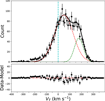
Figure C2. Top panel: the black dots indicate the histogram distribution of the rotational velocity. The red and green dashed lines represent the distributions of the halo and disk components in the model defined in the Bayesian method, respectively. The solid black line represents the distribution of all the stars constrained by the Bayesian method. The cyan vertical line indicates the value 0 for the rotational velocity. Bottom panel: the residual distribution between the histogram distribution of the observational rotational velocity and model.
Download figure:
Standard image High-resolution image