


Abstract
The mass function for black holes and neutron stars at birth is explored for mass-losing helium stars. These should resemble, more closely than similar studies of single hydrogen-rich stars, the results of evolution in close binary systems. The effects of varying the mass-loss rate and metallicity are calculated using a simple semi-analytic approach to stellar evolution that is tuned to reproduce detailed numerical calculations. Though the total fraction of black holes made in stellar collapse events varies considerably with metallicity, mass-loss rate, and mass cutoff, from 5% to 30%, the shapes of their birth functions are very similar for all reasonable variations in these quantities. Median neutron star masses are in the range 1.32–1.37 regardless of metallicity. The median black hole mass for solar metallicity is typically 8–9 if only initial helium cores below 40 (ZAMS mass less than 80 ) are counted, and 9–13 , in most cases, if helium cores with initial masses up to 150 (ZAMS mass less than 300 ) contribute. As long as the mass-loss rate as a function of mass exhibits no strong nonlinearities, the black hole birth function from 15 to 35 has a slope that depends mostly on the initial mass function for main-sequence stars. These findings imply the possibility of constraining the initial mass function and the properties of mass loss in close binaries using ongoing measurements of gravitational-wave radiation. The expected rotation rates of the black holes are briefly discussed.


1. Introduction
A large fraction of massive stars are found in binary systems with sufficiently small separations that interaction is likely sometime in the star's life (Sana & Evans 2011; Kiminki & Kobulnicky 2012; Sana et al. 2012). This interaction will radically affect the sorts of supernovae they produce (Podsiadlowski et al. 1992; Wellstein & Langer 1999; Pols & Dewi 2002; Langer 2012; de Marco & Izzard 2017). Many of the supernovae will no longer be Type II, but Type I. More subtle changes also happen to the core structure that affect the nature of its explosion, including energy, nucleosynthesis, and remnant properties.
Realistic studies of the evolution of stars in binaries can be quite complicated. In addition to the usual uncertainties in mass-loss rates, mixing, rotation, and explosion physics inherent in any study of massive stars, there is the added complexity of mass and angular momentum exchange between the two components. This history depends, in turn, on the initial orbital parameters, mass ratios, efficiency of mass transfer, and the uncertain outcome of common envelope evolution. Kicks may also be important in determining the orbital parameters after each of the two explosions (Vanbeveren et al. 2020).
Using approximations for some of these uncertainties, many previous papers have estimated the properties of the neutron stars and black holes that massive binaries leave behind (e.g., Belczynski et al. 2002, 2012, 2020; Dominik et al. 2012; Fryer et al. 2012; de Mink & Belczynski 2015; Eldridge & Stanway 2016; de Marco & Izzard 2017; Eldridge et al. 2017). While exploring the effects of binary membership quite well, the treatment of the supernova explosion itself was often simplistic in these works. Presupernova models were sometimes adopted from several sources that used different physics to study the evolution. The range of masses considered was often limited and mass loss by winds was treated using prescriptions that, in some cases, have become dated. The role of different assumptions regarding the effects of binary membership was sometimes hard to disentangle.
Here, a different tack is taken (see also Woosley 2019; Ertl et al. 2020). The "model" for binary mass exchange is trivial and not intended as a substitute for more realistic calculations using population synthesis. It is assumed that the chief effect of evolution in a close mass-exchanging system is to remove the hydrogen envelope when the star first attempts to expand to red or blue supergiant proportions. This expansion is assumed to occur near the time of central helium ignition. As a consequence of losing its envelope, the helium core shrinks due to mass loss by a wind rather than growing as hydrogen burns in a surrounding shell. Thus the presupernova stars, in this case the residual cores of helium and heavy elements, are smaller in the "binary" case than for single stars. This result agrees, qualitatively, with the observation that Type Ib and Ic supernovae are more tightly correlated with star-forming regions than Type IIp (Kuncarayakti et al. 2018). Hence they come from stars of greater main-sequence mass. Quantitatively, the results of Woosley (2019) are not so different, for a given main-sequence mass, than those of Yoon et al. (2010), who treated binary evolution more realistically. For example, a 25 solar metallicity main-sequence star leads to a presupernova core mass of 4–6 in Table 1 of Yoon et al. (2010). For Woosley (2019), the presupernova mass is 5.0 . For an isolated 25 star that kept part of its hydrogen envelope until death, the helium core mass would have been 8.4 (Sukhbold et al. 2018). Since the explosion properties and remnant masses depend sensitively on the presupernova core mass, the difference is substantial.


The ansatz of prompt envelope removal facilitates a calculation that otherwise would have been complex and highly parameterized, but also restricts the applicability of the results to just those stars initially close enough to quickly lose their envelopes. We do not treat here stars that would have been Type II supernovae of any sort. Any residual hydrogen is presumed to be promptly lost to a wind. Angular momentum transport is not followed and thus we cannot calculate the final spin of the core (though see Section 4). The complications of uncertain mass loss in extremely massive stars that never become red supergiants, but instead make luminous blue variables, are ignored. Every massive star will have a well-defined helium core mass when it dies, but the relation between that final mass and main-sequence mass is especially uncertain for such stars. We assume the mapping given by Equations (3) and (4) of Woosley (2019). For very high masses the initial helium core mass is roughly half the main-sequence mass.
Perhaps the worst error is ignoring the effect of mass exchange on the initial helium core mass of the secondary. The helium core mass of the secondary, at helium ignition, will be larger than if it had evolved in isolation since it will have accreted some uncertain fraction of its companion's envelope. The secondary may also transfer mass to the compact remnant that resulted from the death of the primary star. The histories of these accretion processes depend on the masses and metallicities of the stars, the orbital parameters, how much mass is lost from the system during any common envelope interaction, and the natal kick of the primary star's remnant. These uncertainties and other characteristics of real binary systems are neglected here. It is assumed that both stars produce presupernova cores defined only by their own initial mass and the adopted mass-loss rate. Consequently, we will underestimate the final masses of half of the stars. Crudely, the effect is that of changing the IMF for the main sequence so as to favor the production of more massive stars, i.e., the effective slope will be be less steep than Salpeter.
With these caveats, what is really studied here is just the remnant mass distributions resulting from a library of mass-losing helium stars whose evolution and explosion were calculated in two previous papers (Woosley 2019; Ertl et al. 2020). A semi-analytic approach to stellar evolution similar to Hurley et al. (2000) is used to estimate the presupernova mass distribution resulting from a given initial distribution of helium core masses at helium ignition. This semi-analytic description gives results in excellent agreement with the full stellar models calculated by Woosley (2019) and can be used to estimate how those results would change for different metallicities and mass-loss prescriptions without running actual stellar evolution calculations. It is further assumed that the remnant mass distribution is uniquely determined by the presupernova masses of the stripped cores, and that mapping is not sensitive to metallicity or interior composition. The mapping is determined from a grid of 1D neutrino-transport models calculated by Ertl et al. (2020). Our study includes the full range of stellar masses expected to produce black holes and most of the stars that make neutron stars. The progenitors of electron-capture supernovae and the results of stellar mergers are omitted.
2. Procedure
To begin, we derive the distribution of presupernova masses for a given initial mass function (IMF), taken here to be Salpeter-like (Salpeter 1955). That is done by integrating the mass-loss equation, , where M is the mass, L is the luminosity, Y is the surface helium mass fraction, and Zinit is the initial metallicity of the star, not counting any newly synthesized heavy elements that appear at the surface later due to mass loss. M, L, and Y vary with time, but not Zinit. For mass loss it is the mass fraction of the iron group that matters most (Vink & de Koter 2005). It is implicitly assumed here that the ratio of iron to other metals remains constant for the range of metallicities considered, chiefly and 0.1 . The initial stars are assumed to be composed of only helium plus Zinit. For solar metallicity the abundances of Lodders (2003) are used, for which the mass fraction of elements heavier than helium is 0.0145 and for iron-group elements (mostly 56Fe) is 0.00147.


Three recent determinations of mass-loss rates for stripped helium stars are considered (Figure 1), taken from Yoon (2017), Vink (2017), and Sander et al. (2020). The work of Yoon is a refinement of earlier empirical fits, while the two studies by Vink and Sander et al. are of a "first principles" nature, based on calculations of radiation transport and hydrodynamics. The former might naturally resemble more observations in the mass range where it is fit while the latter two might be more safely extrapolated to lower mass where the work by Yoon lacks adequate calibration (Gilkis et al. 2019).

Figure 1. Mass loss as a function of luminosity for WN and WC stars of solar and 10% solar metallicity. The expressions plotted are from Yoon (2017, blue), Vink (2017, green), and Sander et al. (2020, red). Blue and red dashed lines are for WN stars, while the Vink rate makes no distinction between WN and WC stars. The rate from Vink has been used, for low values of mass and luminosity, as a lower bound for the rate from Sander et al.
Download figure:
Standard image High-resolution imageYoon gives two formulae for WN and WC stars. For WN stars,

which is taken from Nugis & Lamers (2000). For WC stars, he gives

which is taken from Tramper et al. (2016). Yoon multiples both equations by a factor, fWR, to account for uncertainty, and favors a value fWR = 1.58. Here we treat fWR = 1 as the standard case, but also explore fWR = 2.
Note the explicit dependence in the second equation on Y. This does not reflect the physical role of helium in absorbing radiation, but is an empirical adjustment for the effect of increasing the carbon and oxygen mass fractions. Yoon's formula is strictly valid only for Y < 0.9, but, to good approximation, we can take it to characterize any star that has lost its unburned helium shell.
The rate from Vink (2017) is for optically thin, helium-stripped stars. Designed to reflect stars on the order of 4 , it is possibly a severe underestimate for more massive helium cores at solar metallicity. At lower metallicity, however, the regime of lower-mass loss reflected by Vink (2017) could stretch to much higher masses. Here it is used as a lower bound in all calculations, especially for the Sander et al. (2020) rate, which otherwise goes to very small values at low mass. Nominally for WN-type stars, Vink gives


Sander et al. (2020) give interpolation formulae as a function of L/M for WN and WC stars individually for two different metallicities in their Table 3. See also their Figure 20. In the general case, one would need to interpolate for values of metallicity other than and 0.1 . Here we restrict our survey of Sander et al. rates to just those two values of metallicity. The three mass-loss rates used are plotted as a function of the current luminosity of the helium star for the two metallicities considered in Figure 1. The Vink and Yoon rates are smooth, almost linear functions of the luminosity, while the Sander et al. rate shows a steep cutoff at low luminosity owing to its strong sensitivity to the Eddington parameter. As previously noted, the Vink (2017) is taken as a lower bound to the Sander et al. (2020) mass-loss rate for low luminosity.


To integrate these equations for a given metallicity, one must specify the evolution of the luminosity and surface helium abundance. The latter is also used as a switch to determine whether to use WN or WC mass loss in the cases where two descriptions are given. For higher-mass helium stars, the extent of the helium-burning convective core grows. In the models of Woosley (2019), for low initial mass near 4 , the helium convective core in the presupernova models is only about 52% of the star's mass, but for helium core masses above 50 this fraction increases to near 85% and stays relatively constant. Between 4 and 50 , to reasonable approximation, the fraction is obtained by interpolation,


where is the initial mass of the helium star and is the maximum extent, in mass, of the convective helium core. This mass also marks the transition point for using WC instead of WN rates. Once the processed core is revealed, the surface helium abundance in real stellar models declines rapidly to a minimum value near 0.2 (Table 4 of Woosley 2019). The decline is not precipitous though because the receding helium convective core leaves behind a gradient that the mass loss eventually reveals. Adding this gradient is not a large effect, but its inclusion mildly improves the agreement with the models. Variation of Y from 0.8 to 0.2 only changes the Yoon mass-loss rate by a factor of two and this variation only occurs during a small fraction of the lifetime. Once the current mass of the star, M(t), fell below , we used the approximation


The luminosity history must also be approximated. Fortunately, the luminosity of a helium star during central helium-burning and its lifetime are mostly determined by its current mass and are not very sensitive to how much helium has burned. For example, a 10 helium star evolved without mass loss has a luminosity of 105.15 , 105.21 , and 105.28 after burning 2%, 50%, and 90%, respectively, of the helium in its center. For a 4 helium star, the corresponding numbers are 104.24, 104.32, and 104.34 . Taking the luminosity from only the 50% depletion model thus makes a maximum error in the instantaneous luminosity for most helium abundances of about ∼25%. The average error is less. The helium-burning lifetime is also sensitive to the mass and not much to the metallicity. If, for a given metallicity, the mass-loss rate and the lifetime are functions of only the current mass, then the mass-loss equation can be integrated numerically, for a given initial helium core mass to give the final presupernova mass.


To evaluate the luminosity as a function of mass and the lifetime, a grid of 52 constant-mass helium stars ranging from 2 to 150 was evolved to carbon ignition using the implicit hydrodynamics code KEPLER (similar setup as in Woosley 2019). The luminosity at 50% helium depletion and the total helium-burning lifetime were tabulated for each (Table 1). The mass-dependent luminosity, L(M), drives the evolution of stellar mass, , which was integrated, for a given metallicity and various mass-loss prescriptions. For greater accuracy, the remaining lifetime was varied as the mass of the star decreased. This was accomplished by increasing the time step in proportion to the current remaining lifetime.


Table 1. Constant-mass Helium Stars
| MHe | τ | MHe | τ | ||
|---|---|---|---|---|---|
| () | () | (1013 s) | () | () | (1013 s) |
| 2.0 | 3.47 | 14.2 | 12.5 | 5.39 | 1.85 |
| 2.1 | 3.54 | 12.9 | 13.0 | 5.42 | 1.81 |
| 2.2 | 3.60 | 11.9 | 13.5 | 5.45 | 1.77 |
| 2.3 | 3.66 | 11.0 | 14.0 | 5.48 | 1.74 |
| 2.4 | 3.71 | 10.3 | 16.0 | 5.58 | 1.62 |
| 2.5 | 3.76 | 9.65 | 18.0 | 5.66 | 1.53 |
| 2.8 | 3.88 | 8.00 | 20.0 | 5.73 | 1.45 |
| 3.0 | 3.99 | 7.00 | 22.0 | 5.80 | 1.39 |
| 3.5 | 4.17 | 5.95 | 24.0 | 5.86 | 1.33 |
| 4.0 | 4.32 | 5.04 | 26.0 | 5.91 | 1.30 |
| 4.5 | 4.45 | 4.39 | 28.0 | 5.96 | 1.26 |
| 5.0 | 4.57 | 3.91 | 30.0 | 6.00 | 1.23 |
| 5.5 | 4.66 | 3.54 | 32.0 | 6.04 | 1.20 |
| 6.0 | 4.75 | 3.26 | 34.0 | 6.08 | 1.18 |
| 6.5 | 4.83 | 3.03 | 36.0 | 6.10 | 1.16 |
| 7.0 | 4.90 | 2.84 | 38.0 | 6.14 | 1.14 |
| 7.5 | 4.96 | 2.67 | 40.0 | 6.17 | 1.12 |
| 8.0 | 5.02 | 2.54 | 50.0 | 6.30 | 1.05 |
| 8.5 | 5.07 | 2.42 | 60.0 | 6.41 | 1.00 |
| 9.0 | 5.12 | 2.32 | 66.0 | 6.46 | 0.98 |
| 9.5 | 5.17 | 2.23 | 70.0 | 6.49 | 0.97 |
| 10.0 | 5.21 | 2.15 | 80.0 | 6.57 | 0.94 |
| 10.5 | 5.25 | 2.08 | 90.0 | 6.63 | 0.92 |
| 11.0 | 5.29 | 2.01 | 100.0 | 6.68 | 0.91 |
| 11.5 | 5.33 | 1.96 | 120.0 | 6.78 | 0.88 |
| 12.0 | 5.36 | 1.91 | 150.0 | 6.89 | 0.86 |


Note. Helium stars are evolved at constant mass to build the relation for L(M). The luminosity is evaluated at 50% helium depletion. τ is the time from helium ignition until a central temperature of 5 × 10⁸ K is reached shortly before carbon ignition.
Download table as: ASCIITypeset image
Given the luminosity as a function of mass and the mass-loss rates as a function of luminosity, mass, and metallicity, the mass-loss equation was then integrated. On a laptop this took about a minute for a grid of 30,000 masses between 2.5 and 150 . Four different variations of mass-loss rate and two metallicities were considered. Figure 2 shows a comparison of the semi-analytic results and the presupernova masses derived for actual stellar models using the KEPLER code and Yoon mass-loss rate (Woosley 2019). Errors are small for low and moderate mass-loss rates, but increase slightly for larger values due to the approximate treatment of the surface helium abundance and luminosity in our equations. Both could be improved.


Figure 2. Presupernova masses calculated using the analytic approach described in this paper (solid curve) compared with values for actual stellar models of the same initial mass, metallicity, and mass-loss rate, calculated using the KEPLER code (Woosley 2019, vertical bars). The standard Yoon mass-loss rate (blue) and a value 1.5 times larger (gray) are considered. Inflection points where the curves change slope at around 8 (gray) and 10 (blue) reflect the transition from WN to WC stars.


Download figure:
Standard image High-resolution imageThe resulting presupernova masses are shown for different metallicities and mass-loss rates in Figure 3 for two values of metallicity, solar and 10% solar, and four choices of mass-loss prescription. Smaller values of mass loss were not calculated since the lower limit on the mass loss from Vink already gives presupernova masses essentially equal to the initial mass, i.e., the mass loss was negligible. The Vink results at 10% solar metallicity can thus be used to approximate all smaller values of metallicity, including zero.

Figure 3. Initial and final masses for the mass-loss rates shown in Figure 1. Each color band is bounded on the bottom by solar metallicity and on the top by 10% solar solar metallicity stars. The mass loss is negligible for the Vink rate at 10% solar metallicity.
Download figure:
Standard image High-resolution imageThe second stage of our calculation required mapping these final presupernova masses into the remnant masses produced when their iron cores collapse. This mapping depends, of course, on the uncertain explosion model. For stars that might have some reasonable chance at exploding by the neutrino-driven mechanism, we used the "death matrix" extracted, for the W18 central engine, from the recent work of Ertl et al. (2020). Those calculations followed the outcomes of the core-collapse, by calibrated neutrino-driven explosion models, for a dense grid of presupernova masses from 2.1 to 20 , which correspond to initial helium core masses from 2.5 to 40 . The calculated gravitational masses include the mass decrement due to neutrino losses determined self-consistently using P-HOTB (see Table 3 and Figure 16 of Ertl et al. 2020). Slightly larger values, typically 2% in the gravitational mass, would be obtained using the correction of Lattimer & Prakash (2001).


For higher masses, up to a presupernova mass of 30 , the presupernova stars were assumed to collapse to black holes without an explosion, but with 0.15 subtracted to account for neutrino emission prior to the formation of a black hole. This is consistent with the correction found by Ertl et al. (2020) for their highest-mass models that made black holes "promptly" (i.e., without fallback). Above a presupernova mass of 30 , besides the adjustment for neutrino mass loss, corrections were also made for mass ejected by the pulsational pair instability based on the models from Woosley (2019). For presupernova masses above 60 , his stars exploded and left no remnants.


The resulting remnant masses are given as a function of presupernova mass in Table 2 and Figure 4. As in Ertl et al. (2020), we adopt a maximum baryonic neutron star mass to be 2.75 , which approximately corresponds to a gravitational mass of ∼2.3 . The maximum black hole mass is 46 , as in Woosley (2019). Larger values, up to 56 , could be accommodated for smaller values of the 12C(α, γ)16O reaction rate (Farmer et al. 2019, S. E. Woosley 2020, in preparation). The S-factor used for this critical reaction here was 175 keV b at 300 keV, slightly higher than what was suggested in deBoer et al. (2017).


Figure 4. Gravitational masses of neutron star (green) and black hole (black) remnants as a function of presupernova mass based on the results from Ertl et al. (2020, W18 engine). The presupernova stars were assumed to have solar metallicity and evolved, including mass loss (Yoon 2017), to the presupernova mass shown. The remnant masses were corrected for neutrino mass loss (Ertl et al. 2020). The same correspondence between presupernova mass and remnant mass is assumed to exist for all choices of metallicity and mass-loss prescription.
Download figure:
Standard image High-resolution imageTable 2. The "Death Matrix"
| MpreSN | Mrem | MpreSN | Mrem | MpreSN | Mrem |
|---|---|---|---|---|---|
| () | () | () | () | () | () |
| 2.07 | 1.24 | 5.98 | 1.37 | 10.56 | 1.96 |
| 2.15 | 1.25 | 6.05 | 1.41 | 10.70 | 3.92 |
| 2.21 | 1.25 | 6.12 | 1.42 | 10.81 | 1.76 |
| 2.30 | 1.28 | 6.20 | 1.51 | 10.91 | 2.31 |
| 2.37 | 1.29 | 6.26 | 1.50 | 11.02 | 4.11 |
| 2.45 | 1.26 | 6.33 | 1.48 | 11.13 | 1.86 |
| 2.52 | 1.26 | 6.40 | 1.38 | 11.23 | 2.29 |
| 2.59 | 1.29 | 6.47 | 1.41 | 11.34 | 2.56 |
| 2.67 | 1.30 | 6.54 | 1.40 | 11.44 | 2.23 |
| 2.74 | 1.35 | 6.61 | 1.36 | 11.55 | 6.46 |
| 2.81 | 1.37 | 6.67 | 1.36 | 11.66 | 11.14 |
| 2.88 | 1.38 | 6.74 | 1.36 | 11.88 | 9.52 |
| 2.95 | 1.33 | 6.87 | 1.42 | 12.10 | 11.71 |
| 3.02 | 1.34 | 6.91 | 1.53 | 12.32 | 11.93 |
| 3.09 | 1.33 | 6.95 | 6.42 | 12.54 | 12.17 |
| 3.16 | 1.36 | 6.99 | 6.62 | 12.74 | 11.06 |
| 3.22 | 1.35 | 7.04 | 1.50 | 12.98 | 11.22 |
| 3.29 | 1.34 | 7.10 | 1.58 | 13.21 | 11.06 |
| 3.36 | 1.33 | 7.17 | 1.61 | 13.44 | 13.18 |
| 3.42 | 1.33 | 7.24 | 1.64 | 13.66 | 13.42 |
| 3.49 | 1.39 | 7.33 | 6.80 | 13.89 | 13.68 |
| 3.57 | 1.39 | 7.42 | 1.47 | 14.81 | 14.64 |
| 3.65 | 1.36 | 7.51 | 1.47 | 15.74 | 15.61 |
| 3.73 | 1.38 | 7.61 | 7.08 | 16.68 | 16.54 |
| 3.81 | 1.39 | 7.71 | 1.50 | 17.63 | 17.49 |
| 3.89 | 1.41 | 7.81 | 7.43 | 18.59 | 18.45 |
| 3.98 | 1.43 | 7.90 | 4.88 | 19.56 | 19.41 |
| 4.05 | 1.32 | 8.00 | 7.68 | 20.53 | 20.38 |
| 4.13 | 1.34 | 8.11 | 7.84 | 21.51 | 21.36 |
| 4.21 | 1.56 | 8.21 | 8.00 | 22.50 | 22.35 |
| 4.29 | 1.51 | 8.31 | 8.07 | 23.49 | 23.34 |
| 4.37 | 1.38 | 8.41 | 8.20 | 24.48 | 24.33 |
| 4.44 | 1.42 | 8.47 | 8.25 | 25.49 | 25.34 |
| 4.52 | 1.38 | 8.59 | 8.34 | 26.50 | 26.35 |
| 4.59 | 1.39 | 8.70 | 8.41 | 27.51 | 27.36 |
| 4.67 | 1.41 | 8.80 | 8.50 | 28.52 | 28.37 |
| 4.75 | 1.40 | 8.87 | 8.55 | 29.53 | 29.38 |
| 4.82 | 1.41 | 8.99 | 8.63 | 30.56 | 30.36 |
| 4.90 | 1.64 | 9.09 | 8.72 | 31.57 | 31.35 |
| 4.97 | 1.46 | 9.18 | 8.82 | 32.60 | 32.35 |
| 5.04 | 1.49 | 9.28 | 8.91 | 33.63 | 33.30 |
| 5.12 | 1.36 | 9.38 | 9.01 | 34.66 | 34.08 |
| 5.19 | 1.41 | 9.45 | 9.08 | 36.83 | 36.02 |
| 5.26 | 1.47 | 9.58 | 9.22 | 39.38 | 37.28 |
| 5.34 | 1.49 | 9.67 | 1.41 | 41.95 | 38.02 |
| 5.41 | 1.48 | 9.78 | 1.41 | 44.54 | 38.61 |
| 5.48 | 1.50 | 9.88 | 1.43 | 47.13 | 40.61 |
| 5.56 | 1.50 | 9.98 | 1.45 | 50.22 | 42.78 |
| 5.63 | 1.46 | 10.07 | 1.52 | 52.82 | 45.84 |
| 5.70 | 1.38 | 10.17 | 1.51 | 55.43 | 44.65 |
| 5.77 | 1.44 | 10.29 | 1.52 | 57.42 | 41.20 |
| 5.84 | 1.48 | 10.39 | 1.78 | 60.12 | 3.51 |
| 5.92 | 1.43 | 10.48 | 1.82 |


Note. All remnant masses are gravitational. Presupernova masses below 2.07 were assumed to produce a 1.24 neutron star. The maximum neutron star mass is taken as 2.3 , and presupernova stars above 60.12 left no remnant. The table is largely based on W18 engine results of Ertl et al. (2020).


Download table as: ASCIITypeset image
3. IMF Averaged Birth Functions for Compact Objects
The final stage consisted of weighting the remnant masses with an IMF corresponding to their original main-sequence progenitors. As in Woosley (2019), it was assumed that, for initial main-sequence masses of less than 30 , the helium core mass at the beginning of helium-burning is


For heavier stars

The relation between initial helium star mass and presupernova mass is given in Figure 3.
For a given semi-analytically computed presupernova mass, the corresponding remnant gravitational mass is obtained by interpolating on the relation shown in Table 2 and Figure 4. Any successful supernova explosion that produced a neutron star or a black hole with a fallback mass greater than 10−2 was taken as a fallback case (for details see Ertl et al. 2020). In order to avoid artificial structures in the birth function, we do not interpolate between fallback and non-fallback cases, i.e., only interpolate if the nearest two grid points in Table 2 are either both fallback, or both non-fallback.

3.1. Neutron Stars
Combining these results, the birth function and its properties for neutron stars are illustrated in Figure 5 and Table 3. A Salpeter-like IMF with α = 2.35 was assumed over the entire mass range (Section 2). The distribution for solar metallicity and mass-loss rates from Yoon (2017) agrees very well with the results based on actual stellar models in Ertl et al. (2020). The median gravitational mass for fWR = 1, i.e., 1.35 , is also within 0.01 of their result. Perhaps this is not surprising given that most of Table 2 was extracted from that work, but it does validate the calculation of presupernova masses by simply numerically integrating the mass-loss history.


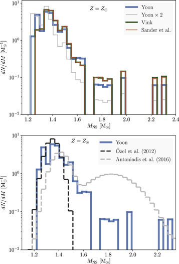
Figure 5. Given the presupernova masses (Figure 3) for helium stars with solar metallicity evolved with mass loss (Figure 1), the remnant masses can be calculated from the data in Figure 4 and Table 2. The normalized birth function for the gravitational neutron star mass is shown here in the top panel for four choices of mass-loss rate: Yoon (2017, blue), Vink (2017, green), Sander et al. (2020, red), and twice Yoon (2017, gray). The birth function is quite robust against changes in the mass-loss rate. Median values range from 1.32 to 1.37 , while the fractions of supernovae range from 90% to 69% between twice the Yoon's and Vink's prescriptions, respectively. The bottom panel compares the case of Yoon mass loss with fWR = 1 with observations by Özel et al. (2012) and Antoniadis et al. (2016).

Download figure:
Standard image High-resolution imageTable 3. Average Neutron Star Masses
| M0.45 | Median | M0.55 | fNS | |
|---|---|---|---|---|
| () | () | () | ||
| Zinit = | ||||
| Yoon | 1.341 | 1.349 | 1.359 | 0.784 |
| Yoon × 2 | 1.314 | 1.320 | 1.326 | 0.907 |
| Vink | 1.360 | 1.368 | 1.376 | 0.686 |
| Sander et al. | 1.360 | 1.368 | 1.376 | 0.684 |
| Zinit = 0.1 | ||||
| Yoon | 1.355 | 1.364 | 1.372 | 0.700 |
| Yoon × 2 | 1.349 | 1.357 | 1.366 | 0.715 |
| Vink | 1.361 | 1.369 | 1.378 | 0.683 |
| Sander et al. | 1.361 | 1.369 | 1.377 | 0.677 |


Note. All quantities are evaluated with Salpeter α = 2.35 across the entire helium star mass range. M0.45 and M0.55 are mass points where the normalized fraction of neutron stars is 45% below and above, respectively. fNS is the fraction of supernova explosions that form neutron stars.
Download table as: ASCIITypeset image
Figure 5 and Table 3 additionally show, however, a weak dependence of the distribution function on mass loss. For instance, the frequency of the most massive neutron stars (>1.7 ), made by fallback in more massive progenitors (Ertl et al. 2020), is reduced with stronger mass-loss rate. For the low mass-loss rate from Vink (2017) the median neutron star mass is 1.37 and for the high mass-loss rate, twice that of the standard value of Yoon (2017), the mass is 1.32 . We thus predict that the median gravitational mass of neutron stars in binary systems will vary, but only a little, with mass loss—and hence with metallicity.


This agreement belies the fact that the total number of neutron stars is substantially different in the three cases. In each case, the distribution function has been normalized so that the integral of number over mass is unity. For the upper limit mass-loss rate (Yoon with fWR = 2), the fraction of core collapses that produce a neutron star is 90%, while for the lower limit mass-loss rate (Vink's) it is only 69% since many more stars remain massive enough to collapse into black holes.
Figure 5 also shows the comparison with the standard case of Yoon mass-loss rates with fWR = 1 and observationally inferred distributions by Özel et al. (2012) and Antoniadis et al. (2016). For neutron star gravitational masses below 1.5 , which are the bulk of the observed objects, our model agrees well with both works though better with Özel et al. (2012). We also agree with Antoniadis et al. (2016) on the existence of a heavier component above 1.5 that, in our case, results from fallback during the explosion. However, we produce far fewer massive objects than claimed by Antoniadis et al. (2016). Possible explanations are an underestimate of fallback in our models or additional accretion by the neutron star during the spin-up phase. This heavier component is derived by Antoniadis et al. (2016) from observations of millisecond pulsars.


3.2. Black Holes
In a similar fashion, the birth function for black holes can be calculated and is also found not to vary greatly with metallicity or mass-loss prescription. A caveat is that it has been assumed that helium cores all the way up to 150 , hence ZAMS stars to 300 are produced with the same continuous Salpeter-like mass function. If star formation is truncated at a smaller mass, this would appear as a cutoff in the black hole mass distribution. If, for example, no stars formed in close binaries with main-sequence masses over 100 , there would be no helium cores with initial mass over 44 . Hence for solar metallicity and standard Yoon mass-loss rates, there would be no presupernova masses over 22 and no black holes heavier than that either. Mass loss for extremely massive stars at a rate very different from the unverified extrapolation of the expressions used here, would also give different, interesting results.


The remnant mass distribution for black holes is shown in Figure 6, and its properties are listed in Table 4 assuming that the mass range of initial helium cores extends from 2.5 to 150 or 2.5 to 40 . The lower value corresponds to a still quite massive main-sequence star and is the limit of the Ertl et al. (2020) survey. Besides the medians, which are not very precisely determined due to the irregular shape of the distribution, the limits M0.45 and M0.55 are also given. These are the masses above and below which 45% of the black holes have their masses. Helium star ranges from 2.5 to 40 and 2.5 to 150 correspond to upper limits of the main-sequence mass function, around 100 and 300 , respectively. For the more limited mass range, the median black hole mass using standard Yoon mass loss (fWR = 1) at solar metallicity and the W18 central engine, which was used to make Table 2, is 8.6 . This is in excellent agreement with the 8.6 calculated by Ertl et al. (2020) using the same assumptions, but actual stellar models, serving again to validate the semi-analytic approach used here, i.e., the use of Table 1 to integrate the mass-loss equation to estimate presupernova masses without running actual stellar models. For the larger mass range, including helium stars up to 150 , the results differ, though not greatly. Ertl et al. (2020) gave a median black hole mass of 10.9 for the W18 engine. We get 11.3 . The new value is slightly larger and more accurate because pulsational pair-instability supernovae (PPISN) were not included in the previous study.


Figure 6. The black birth function for solar metallicity (top) and 10% solar metallicity (bottom) stars using the presupernova masses given in Figure 3. The birth function is not very sensitive to the mass-loss prescription and metallicity. It is bounded on the lower end by the maximum-mass neutron star and on the upper end by the onset of PPISN. There is no unpopulated "gap" between neutron stars and black holes. The gap near 10 is due to the presupernova compactness variation, and the pile-up at high mass is due to PPISN. At low metallicity, the Sander et al. prescription predicts a well-defined pile-up near 20 . The peak of the distribution is broadly consistent with that inferred from X-ray binary systems (e.g., Özel et al. 2010; Farr et al. 2011), and the range at high mass encompasses all currently known BH merger events from LIGO/Virgo within the 90% confidence level.


Download figure:
Standard image High-resolution imageTable 4. Average Black Hole Masses
| M0.45 | Median | M0.55 | fBH | |
|---|---|---|---|---|
| () | () | () | ||
| () | ||||
| Yoon | 8.4 | 8.6 | 8.9 | 0.17 |
| Yoon × 2 | 7.8 | 7.9 | 8.0 | 0.04 |
| Vink | 13.2 | 14.2 | 15.2 | 0.30 |
| Sander et al. | 8.4 | 8.6 | 8.9 | 0.29 |
| Yoon | 12.1 | 13.7 | 14.6 | 0.27 |
| Yoon × 2 | 10.9 | 11.8 | 13.3 | 0.24 |
| Vink | 13.6 | 14.5 | 15.6 | 0.30 |
| Sander et al. | 13.6 | 14.5 | 15.6 | 0.30 |
| () | ||||
| Yoon | 9.5 | 11.3 | 13.1 | 0.22 |
| Yoon × 2 | 11.5 | 13.2 | 14.3 | 0.09 |
| Vink | 14.3 | 15.5 | 16.8 | 0.31 |
| Sander et al. | 8.7 | 9.1 | 10.9 | 0.32 |
| Yoon | 14.1 | 15.3 | 16.5 | 0.30 |
| Yoon × 2 | 13.5 | 14.5 | 15.6 | 0.29 |
| Vink | 14.5 | 15.7 | 17.0 | 0.32 |
| Sander et al. | 14.7 | 16.0 | 17.3 | 0.32 |
| Zinit = | ||||
| Yoon (α = 1.35) | 16.4 | 18.1 | 20.0 | 0.47 |
| Yoon (α = 1.85) | 13.3 | 14.5 | 15.9 | 0.33 |
| Yoon (α = 2.35) | 9.5 | 11.3 | 13.1 | 0.22 |
| Yoon (α = 2.85) | 8.5 | 8.9 | 10.5 | 0.14 |
| Yoon (α = 3.35) | 8.2 | 8.4 | 8.6 | 0.08 |


Note. All masses include correction to neutrino emission. M0.45 and M0.55 are mass points where the normalized fraction of black holes is 45% below and above, respectively. fBH is the combined fraction of implosions and supernovae that form black holes.
Download table as: ASCIITypeset image
The shape of the birth function (Figure 6) is not very sensitive to either metallicity or mass-loss rate. Note that all distributions have been normalized so that the integral of dN/dM over all black hole masses is one. As in Ertl et al. (2020), a few low mass black holes are made by fallback and there is a narrow gap of production around 10 . The exact location of this gap will be sensitive to the compactness distribution of the presupernova stars and thus may vary with different choices for convection theory and 12C(α, γ)16O reaction rate, but its presence is robust and worth looking for, as it would provide constraints on the presupernova evolution. The birth function for black holes left by PPISN, i.e., masses 35–46 , is noisy. Whether this reflects the sparse sample of PPISN used to generate the plot (Table 5 of Woosley (2019) has a resolution in black hole mass of about 2 ) or a physical effect needs further investigation. Current results suggest a preponderance of black holes with masses 35–40 . This is because the more massive PPISN near the upper limit (46 here) have more violent instabilities and eject more mass.


The relatively small values for the median black hole mass using the Sander et al. mass-loss rate at solar metallicity are a consequence of the pile-up in presupernova masses around 8–10 , resulting from the very nonlinear decrease in the mass-loss rate at around a luminosity of 105.2 (Figure 1 and Table 1). At lower metallicity the dip in mass loss occurs at higher mass and also less mass is lost, so the effect on the median mass is not so great.


The median black hole masses when the entire mass range of initial helium core masses, 2.5–150 , is sampled, are substantially larger than what is frequently cited by observers for binary X-ray sources. Özel et al. (2010) gives a mean mass of 7.8 ± 1.2 . A similar value was found, in the case of a single Gaussian fit, by Farr et al. (2011). This lower value could reflect a cutoff in the production of very high mass stars coupled with a high mass-loss rate, or observational bias. X-ray binaries containing black holes above 20 (resulting from initial helium core masses over 40 and main-sequence masses over 80 ) may be rare, short lived, and difficult to detect. Wyrzykowski et al. (2016) have studied 13 candidate compact objects using microlensing. The maximum-mass black hole they observed had a mass of about 9 plus or minus a factor of two. Given the sparse sample and large error bar, this is consistent with our predictions. They also found no evidence for a mass gap between neutron stars and black holes. LIGO/Virgo turned up a large sample of much heavier black holes (Abbott et al. 2019). This might be regarded as a more complete census of the stellar graveyard for very high mass stars, since the black holes that are merging might not be easily detected any other way.


The fraction of core collapses that produce black holes is sensitive to the mass-loss rate employed. For a bigger mass-loss rate, a black hole of given mass comes from a higher-mass, rarer main-sequence star. For the full range of helium core masses considered, our computed fraction ranges from 9% to 32% (Table 4), which is consistent with a prior estimate by Kochanek (2015)–9% to 39%. When the sampling interval is restricted to initial helium core masses below 40 , however, our fraction is smaller, as little as 4% for Yoon mass-loss rates with fWR = 2. The maximum limit, regardless of metallicity is 30%.

An important feature in our results is the nearly constant slope of the black hole birth function roughly between 15 and 35 . Above 35 , the distribution is altered by the PPISN, while below 15 stars frequently produce supernovae, and thus the distribution is highly modular due to the varying outcomes of the stellar collapse. In between lies a prominent range where the black hole mass is solely determined by the presupernova mass, minus the small correction for neutrino emission. If the mass-loss rate has no rapid change in slope in this mass range, the birth function will be smooth and if the dependence on mass nearly linear, it will mirror the stellar IMF. For solar metallicity, the Vink and Yoon mass-loss rates satisfy these criteria and the birth function in Figure 7 is smooth. For lower metallicities, the differing dependencies on Zinit of the rates for WN and WC mass loss cause a spike whose location migrates with the changing Zinit.


Figure 7. Dependence of the black hole birth function on the metallicity for the Yoon mass loss rates with fWR = 1 (top panel) and 2 (bottom panel). Globally, the shape of the birth function does not depend sensitively on metallicity though the number of black holes does (Table 4). Note that each distribution is normalized so that the area beneath is one. The sharp peak seen for some cases between 15 and 35 , and most pronounced for the high mass-loss case in the lower panel, is due to a pile-up of masses at the transition mass, MWN–WC, where the Yoon mass-loss rate abruptly changes slope. See the insets in Figures 1 and 2. The sharpness of these peaks is artificial since the mass-loss rate does not truly change slope abruptly and the observed black holes will not all come from progenitors with a single metallicity. Note the lack of any peaks in the 15–35 mass range for Zinit > 0.3 for the standard Yoon rate, and at Zinit > 0.1 for twice the Yoon rate.


Download figure:
Standard image High-resolution imageThe spike is due to a "flat spot" in the presupernova mass resulting from the transition from WN to WC mass loss (Figure 2). Its sharpness and location are probably an artifact of the empirical mass-loss description for the two cases, which lead to a significant jump between the WN and WC mass-loss when evaluated at lower metallicities. Such a significant jump in mass-loss rate between the WN and WC stage is probably not realistic. In any case, the observed distribution would be smoother, as it would never include just one metallicity, but a range. The Sander et al. (2020) rate also exhibits a similar spike at low metallicity, but for a different reason. For 0.1 , the mass-loss rate is very nonlinear for a luminosity of 105.8 , corresponding to a mass near 20 (Figure 1 and Table 1). This ledge has a physical basis, namely the strong dependence of the Sander et al. rate on the Eddington Gamma-factor, Γe, essentially the ratio of acceleration due to Thomson scattering and gravity (Vink 2006; Sander et al. 2015). A signature in the black hole IMF would thus have interesting implications for the theory of stellar mass loss.


The fact that, for solar metallicity at least, the slope of the birth function between 15 and 35 in Figure 6 is nearly constant for other choices of mass-loss rate, reflects the near linear relation between and M in that mass range (see Figure 1 and Table 1). Due to the Eddington limit, the lifetime of very massive stars is nearly constant at τ ≈ 300,000 yr, so the presupernova mass is almost a constant fraction of the initial helium core mass:


where k is positive and defined by . Since all stars in this mass range are assumed to collapse to black holes with gravitational masses very nearly equal to presupernova masses, this means that the remnant mass is a constant times the ZAMS mass, though the value of that constant will vary with metallicity and mass-loss rate. Consequently, the slope of the birth function is mostly sensitive to the IMF for massive stars (Figure 8). Measuring the BH birth function in this mass range with LIGO/Virgo offers an opportunity to determine this important quantity. The corresponding mass range sampled on the main sequence depends on the mass-loss rate employed and can be read from Figure 3 for the initial helium star mass to be used in Equations 6 and 7. For solar metallicity and standard Yoon loss rates, the main-sequence mass range sampled would be approximately 70–150 . Sparse data currently exist for main-sequence stars with these masses due to their small birth numbers and short lifetimes.


Figure 8. The top panel shows the sensitivity of the black hole birth function to the assumed initial mass function for main-sequence stars in close binaries for the standard Yoon mass-loss rate and several choices for the Salpeter power-law exponent, α. The value α = 2.35 is standard. The lower panel shows the dependence of the slope on both α and metallicity for the standard Yoon mass-loss prescription for a region of mass where all presupernovae are assumed to collapse to black holes with no mass loss except for what neutrinos carry away.
Download figure:
Standard image High-resolution imageIn the more general case that , with ν not equal to 1, the presupernova mass for very massive stars with constant lifetime τ is


For ν > 1 this implies an upper limit to the mass of black holes of

For ν < 1 there is no upper bound and the final black hole mass continues to increase monotonically so long as helium cores of arbitrarily high mass are produced. For the mass-loss rates considered here, ν above 100 is so close to 1 that this upper limit is much larger than the range considered here. For larger mass-loss rates and larger ν though, this limit could be important. For example, the mass-dependent mass-loss rate of Langer (1989), y−1, gives Mmax = 8 . For solar metallicity, there would be no black holes with greater mass, no matter how big the masses on the main sequence were.


4. Discussion and Conclusions
Using simple approximations to binary evolution and supernova explosions, the birth functions for neutron stars and black holes have been calculated for a variety of metallicities and modern mass-loss rates. The evolution captures the essential nature of a helium star that shrinks due to mass loss after losing its envelope, rather than a helium core growing in a single star. The explosion model assumes that the outcome, at least in terms of remnant mass, is determined by the presupernova core mass independent of metallicity or interior structure and composition. The presupernova mass is determined by integration of the mass-loss equation, not by computing actual stellar models. Within this framework a large set of results can be quickly computed and general trends determined.
The results (Tables 3 and 4; Figures 5–7) show patterns that, to good approximation, are independent of mass-loss rate and metallicity. Neutron stars of all gravitational masses from 1.23 to the maximum mass, here assumed to be 2.3 , are produced. The distribution has a central peak near 1.35 , with rare events producing much heavier neutron stars by fallback (see also Ertl et al. 2020). Increased mass loss decreases the proportion of the most massive members (Figure 5).


The black hole birth function has four parts (Figure 6). A low-mass tail below 5 , produced entirely by fallback in explosions that initially make a neutron star, is followed by a broad distribution resulting from both direct implosions and explosions with massive fallback. This distribution has a pronounced peak around 8–9 . Its irregularity from 5 to 12 reflects the mixed distribution of stars that explode leaving neutron stars or implode into black holes. There is a hint of a gap around 10 due a local minimum in the core compactness parameter for that presupernova mass (Woosley 2019; Ertl et al. 2020). The location of this gap may depend on uncertainties in presupernova evolution like the 12C(α, γ)16O reaction rate. Above 12 , in the present prescription, all presupernova cores collapse promptly to black holes and the distribution reflects the IMF for the original stars modulated by any rapid nonlinear behavior of the mass-loss rate. Nonlinearity can result from an abrupt transition between WN and WC mass-loss formulae (Yoon 2017), or a rapid cutoff below a certain Eddington factor (Sander et al. 2020). The mass where the inflection occurs is sensitive to the mass-loss rate and metallicity (Figure 7) and might be spread out by observations that span a range in metallicities. Without this structure, which is weak or absent in the case of smooth (Vink 2017) or small mass loss, the slope of the black hole birth function mirrors that of the stellar IMF between about 15 and 35 (Figure 8). From 35 to 46 , there is a pile-up of PPISN remnants. More massive PPISN eject more mass, so there is a peak around 38 . The location of the peak and the cutoff mass will be sensitive to the rate for 12C(α, γ)16O. All birth functions were calculated assuming the continuation of a Salpeter-like IMF to helium core masses as large as 150 . This corresponds to a ZAMS mass of about 300 . Any sharp variation in the IMF for lower masses would imprint structure in the black hole birth function.


While our survey has used a range of mass-loss rates from the recent literature, observational constraints and spectral analysis of Wolf–Rayet (WR) stars point toward high mass-loss rates such as described by the empirically motivated recipe of Yoon (2017). The number ratio of observed Type WC and WN stars and the ejected masses of Type Ic supernovae require that sufficient mass-loss occurs, especially at solar metallicity, to frequently uncover the carbon–oxygen core (Conti 1976) before the star dies.
Neugent & Massey (2011) report a ratio of massive WC to WN stars that ranges from 58% at solar metallicity to 9% for the Small Magellanic Cloud (SMC, roughly /5). Neugent & Massey (2019) give similar values, 0.83 ± 0.10 for the Milky Way and 0.09 ± 0.09 for the SMC. Rosslowe & Crowther (2015) give a range from 0.51 ± 0.08 to 0.40 ± 0.16 for the inner and outer Milky Way, respectively. Table 5 shows our corresponding numbers for the standard Yoon, twice the Yoon, and Sander et al. rates, each using Equation (4) for the transition mass. The theoretical fractions have been evaluated using the IMF (α = 2.35) weighted average of the time spent by each set of models as a WC or WN star.

Table 5. WC/WN Ratios
| Z | Observed | Yoon | Yoon × 2 | Sander et al. | Cut-off |
|---|---|---|---|---|---|
| 0.5–0.8 | 0.05 | 0.15 | 0.02 | ||
| 0.12 | 0.42 | 0.06 | |||
| 0.33 | 1.74 | 0.14 | |||
| 0.49 | 1.30 | 0.15 | |||
| /5 | ∼0.1 | 0.01 | 0.03 | ⋯ | |
| 0.02 | 0.08 | ⋯ | |||
| 0.20 | 0.98 | ⋯ | |||
| 0.26 | 0.99 | ⋯ |


Note. "Observed" values are from Neugent & Massey (2011). The SMC is taken to be 0.2 . No fits for or interpolation formulae for 0.2 were given by Sander et al. (2020). WC/WN ratios obtained using the rates of Vink (2017) were much smaller.


Download table as: ASCIITypeset image
The model results depend upon the mass or luminosity range one ascribes to stars that are, observationally, WR stars. This range depends upon metallicity. For example, according to Shenar et al. (2020), only helium stars above will be, spectroscopically, classical WR stars in our present Galaxy (see also Sander et al. 2019). For the Large and Small Magellanic Clouds, Shenar et al. (2020) give larger, and 5.6 (see also Hainich et al. 2014). By this criterion, the rest of our helium stars would be "stripped stars", but not WR stars. We thus evaluated our average WC/WN ratios for several cutoffs, three given by initial helium core mass and one by the luminosity of the star as it evolved. The mass cutoffs considered were 2.5 (initial ); 4 (initial ), and, for the two metallicities, either 7 (initial ) or 16 (initial ). In the fourth case each star was only considered to be a WR star during the time its luminosity exceeded the threshold given by Shenar et al. (2020). In this, and the higher-mass cutoff cases, a much smaller fraction of stripped stars are WR stars. Most of the ones excluded are WN stars, so the WC/WN ratio is increased.


Many possible sources of error enter the comparison in Table 5. Not all the observed WR stars were stripped by binary mass exchange. The definition of a transition mass (Equation (4)) is approximate and arbitrary. The observed lower luminosity for classical WR stars is approximate. If the cutoff is reduced from –5.25 in the case of the SMC, the ratio of WN/WC stars for our models drops from 0.22 to 0.12 for the standard Yoon mass loss rates. More realistic studies show good agreement, for the mass-loss rates they assume (Vanbeveren et al. 2007; Eldridge et al. 2017). Still, our simple results suggest that mass loss rates near those given by Yoon (2017), with a multiplier fWR between 1 and 2, are favored over smaller ones. Following similar arguments, Yoon (2017) himself suggested 1.58. The Vink (2017) and Sander et al. (2020) rates produce too few WC stars.

A similar conclusion comes from considering SN Ib and SN Ic progenitor masses. Using the Yoon rates with fWR = 1 gives a critical presupernova mass separating WN progenitors from WC progenitors near 7.0 (Woosley 2019). Increasing the rate by a factor of 1.5 reduces that critical mass to 4.9 , and a new calculation using the KEPLER code shows that using fWR = 2 lowers the critical mass to 3.9. Assuming 1.5 is left in the neutron star, this implies ejected masses of 5.5, 3.4, and 2.4 , respectively. Measured average ejected masses for Type Ic supernovae are near 2.2 (Prentice et al. 2019), suggesting fWR = 2 might be appropriate. Again there are caveats. It is not clear that the production of a Type Ic supernova requires the complete loss of the helium shell (Dessart et al. 2012).


Using Yoon's rates with fWR = 2 gives a median neutron star mass at solar metallicity of 1.32 (1.35 if the Lattimer & Prakash 2001 correction for neutrino losses is employed instead of the value calculated by Ertl et al. 2020), and a median black hole mass of 7.9 , for initial helium cores with smaller initial mass than 40 (ZAMS mass less than 80 ). Given the small fraction of black holes predicted by this cutoff (Table 4) and the small maximum black hole mass implied (11.1 from a presupernova of 11.7 ; Figure 3 and Table 2), it may not be realistic to truncate the maximum initial helium core mass at such a low value if the mass-loss rate is this large. The median black hole mass including all initial helium star masses up to 150 is 13.2 . In all cases, the maximum presupernova mass to collapse and leave a remnant is 60 and the maximum black hole mass, following pulsational activity, is 46 (Woosley 2019, Figure 6).


The formalism developed here is simple and easily applicable to more realistic descriptions of binary evolution (e.g., Dominik et al. 2012; Fryer et al. 2012; Spera et al. 2015; Eldridge et al. 2017; Vigna-Gómez et al. 2018). Once the helium core is uncovered the mass-loss equation is easily integrated and the remnant mass is determined using Tables 1 and 2. Indeed, our results are not only applicable to binary mass exchange. By adjusting the lifetime in Table 1 to reflect the actual duration of the WR phase, presupernova masses can also be calculated for single stars, and stars that experience chemically homogeneous evolution (e.g., de Mink & Mandel 2016). Unless that adjustment is large, the results presented here, nominally for close binaries, should be robust. The main-sequence masses used in weighting the contributions in an IMF average would also need to be adjusted as in Equations 6 and 7 or their equivalents.
While this paper is about simple one-dimensional models, it is possible to make some inferences about the rotation rates for the black holes that are produced. This is because the final angular momentum is very sensitive to the amount of mass lost by the helium core during the stripped phase. The initial angular momentum of the helium core can be quite large. A fit, to 5% accuracy, to the radii of the helium star models of Woosley (2019) after they have burned only 1% of their helium to carbon, is cm. The moment of inertia of a n = 3 polytrope, which these stars resemble, is 0.0754 MR2 (Criss & Hofmeister 2015), though a slightly better fit to the models will be used here, 0.09 MR2. If the helium star initially rotates with surface velocity equal to a fraction fKep of Keplerian, , then the initial angular momentum will be


The Kerr parameter for the initial helium star, on the other hand, is

For rapid but not extreme rotation the helium core can begin its life with sufficient angular momentum to make a Kerr black hole. fKep = 0.33 corresponds to a ratio of centrifugal force to gravity of 10%, which might be achieved by chemically homogeneous evolution (Woosley & Heger 2006).
As the star loses mass though, it loses angular momentum. About 80% of the angular momentum in the initial rigidly rotating star is contained in the outer half of its mass. This fraction is amplified appreciably by transport, especially by magnetic torques, as the star burns helium. In practice, no helium star that begins with reasonable rotation and loses half or more of its mass will produce a Kerr hole. This includes all the models presented here that make black holes using mass loss rates from Yoon (2017) with fWR = 1 or 2 at solar metallicity. In fact, following transport in an actual KEPLER model using the physics described in Woosley & Heger (2006) for a helium core with initial mass 60 and final mass 30 (fWR = 1; Yoon rates) shows that losing half the mass reduces the angular momentum by a factor close to 100. Approximately the same reduction is also observed in a 30 star that loses half its mass. One thus expects Kerr parameters a ≲ 0.1 for the black holes resulting, even for stars with rapid initial rotation, from use of the Yoon rates at solar metallicity. The Kerr parameter would be substantially larger though at lower metallicity, especially if the rates of Vink or Sander et al. are employed (Figure 3). Had the same 30 model lost only 5 instead of 15 , it would have made a 25 black hole with a = 1.


These qualitative arguments agree with the results of more detailed studies (e.g., Belczynski et al. 2020). Unless the mass loss is small, the spins of merging massive binary black holes are likely to be small.
We thank the anonymous referee for many useful suggestions and references that helped to improve this work. The authors acknowledge extensive, educational correspondence with Andreas Sander on the topic of mass loss in massive helium stars. He, Jorick Vink, and Sung-Chul Yoon made numerous suggestions that resulted in an improved manuscript. We also thank Carolyn Raithel for providing observationally inferred compact object mass distribution data. This work has been partly supported by NASA NNX14AH34G. T.S. was supported by NASA through a NASA Hubble Fellowship grant #60065868 awarded by the Space Telescope Science Institute, which is operated by the Association of Universities for Research in Astronomy, Inc., for NASA, under contract NAS5-26555. At Garching, funding by the European Research Council through Grant ERC-AdG No. 341157-COCO2CASA and by the Deutsche Forschungsgemeinschaft (DFG, German Research Foundation) through Sonderforschungsbereich (Collaborative Research Centre) SFB-1258 "Neutrinos and Dark Matter in Astro- and Particle Physics (NDM)" and under Germany's Excellence Strategy through Cluster of Excellence ORIGINS (EXC-2094)—390783311 is acknowledged.