


Abstract
We calculate the evolution of massive stars, which undergo pulsational pair-instability (PPI) when the O-rich core is formed. The evolution from the main sequence through the onset of PPI is calculated for stars with initial masses of 80–140 M⊙ and metallicities of Z = 10−3−1.0 Z⊙. Because of mass loss, Z ≤ 0.5 Z⊙ is necessary for stars to form He cores massive enough (i.e., mass >40 M⊙) to undergo PPI. The hydrodynamical phase of evolution from PPI through the beginning of Fe-core collapse is calculated for He cores with masses of 40−62 M⊙ and Z = 0. During PPI, electron–positron pair production causes a rapid contraction of the O-rich core, which triggers explosive O-burning and a pulsation of the core. We study the mass dependence of the pulsation dynamics, thermodynamics, and nucleosynthesis. The pulsations are stronger for more massive He cores and result in a large amount of mass ejection such as 3–13 M⊙ for 40−62 M⊙ He cores. These He cores eventually undergo Fe-core collapse. The 64 M⊙ He core undergoes complete disruption and becomes a pair-instability supernova. The H-free circumstellar matter ejected around these He cores is massive enough to explain the observed light curve of Type I (H-free) superluminous supernovae with circumstellar interaction. We also note that the mass ejection sets the maximum mass of black holes (BHs) to be ∼50 M⊙, which is consistent with the masses of BHs recently detected by VIRGO and aLIGO.
1. Introduction
1.1. Pulsational Pair-instability (PPI)
The structure and evolution of massive stars depend on stellar mass, metallicity, and rotation (e.g., Nomoto & Hashimoto 1988; Arnett 1996; Heger et al. 2000; Heger & Woosley 2002; Nomoto et al. 2013; Hirschi 2017; Limongi 2017; Meynet & Maeder 2017). In stars with the zero-age main-sequence (ZAMS) mass of M ∼ 10 – 80 M⊙, hydrostatic burning progresses from light elements to heavy elements in the sequence of H, He, C, O, Ne, and Si burning, and finally an Fe core forms and gravitationally collapses to form a compact object, such as a neutron star.
For very massive stars with M ≳ 80 M⊙ (i.e., an He core of mass greater than 35 M⊙), although exact correspondence is strongly dependent on metallicity (El Eid et al. 1983; Heger & Woosley 2002; Hirschi 2017; Woosley 2017), the effects of electron–positron pair production () on stellar structure and evolution are important when the O-rich core is formed (Fowler & Hoyle 1964; Fraley 1968). Pair production causes the dynamically unstable contraction of the O-rich core, which ignites explosive O-burning. For 140 M⊙ ≲ M ≲ 300 M⊙, the nuclear energy released is large enough to disrupt the whole star, so that the star explodes as pair-instability supernovae (PISN) (Barkat et al. 1967; Bond et al. 1984; Baraffe et al. 2001). Above ∼300 M⊙, the star collapses to form a black hole (BH) again. As a result, no BH can be formed with a mass between ∼50 M⊙ and ∼150 M⊙ (Heger & Woosley 2002). Such a mass gap may provide distinctive features in the mass spectrum of BHs through the detection of a merger event of binary BHs.

For stars with (He cores of 35 to ∼65 M⊙, Woosley 2017), explosive O-burning does not disrupt the whole star, but creates strong pulsations (Barkat et al. 1967; Rakavy & Shaviv 1967), which is called PPI. These stars undergo distinctive evolution compared to more massive or less massive stars. PPI is strong enough to induce massive mass ejection as in PISNe, while the star further evolves to form an Fe core that collapses into a compact object later as a core-collapse supernova (CCSN). PPI supernovae (PPISNe) of 80−140 M⊙ stars are thus the hybrid of a PISN and a CCSN.

The exact ZAMS mass range of PPISNe depends on the mass loss by stellar wind, thus on metallicity, and also on rotation. For PPISN progenitors, the wind mass loss during H- and He-burning phases could contribute to the loss of almost a half of the initial progenitor mass (see, e.g., Table 2 of Woosley 2017). Such mass loss can suppress the formation of a massive He core. The exact mass of the He core as a function of metallicity and ZAMS mass remains less understood because the mass loss processes in massive stars are not well constrained (Renzo et al. 2017). Rotation provides additional support by the centripetal force, which allows PPISNe to be formed at an even higher progenitor mass (Glatzel et al. 1985; Chatzopoulos & Wheeler 2012).
In order to pin down the mass range of PPISNe, a mass survey of main-sequence star models is done in Heger & Woosley (2002) and Ohkubo et al. (2009) with focus on zero-metallicity stars. Large surveys at other metallicities can be also found in, e.g., Heger & Woosley (2010) and Sukhbold et al. (2016). A large array of stellar models covering also PPISNe with rotation has been further explored in Yoon et al. (2012).
The evolution of a PPISN is very dynamical in the late phase. During the pulsation, the dynamical timescale can be comparable with the nuclear timescale when the hydrostatic approximation is no longer a good one. Also, when the star drastically expands after the energetic nuclear burning triggered by the contraction, the subsequent shock breakout near the surface is obviously a dynamical phenomenon. This suggests that during this dynamical but short phase, hydrodynamics instead of hydrostatics is required in order to follow the evolution consistently. Unlike hydrodynamical studies of PISNe (Barkat et al. 1967; Heger & Woosley 2002; Umeda & Nomoto 2002; Scammapieco et al. 2005; Chatzopoulos et al. 2013; Chen et al. 2014), a systematic hydrodynamical study of PPI has been conducted only recently (e.g., Woosley & Heger 2015; Woosley 2017).
1.2. Connections to Observations
The optical aspect of PPI and PPISNe might explain some superluminous supernovae (SLSNe), such as SN2006gy (Woosley et al. 2007; Kasen et al. 2011; Chen et al. 2014). Recent modeling of SLSN PTF12dam (Tolstov et al. 2017) has required an explosion of a 40 M⊙ star with a 20–40 M⊙ circumstellar medium (CSM) with a total of 6 M⊙ 56Ni in the explosion. The shape, rise time, and fall rate of the light curves of such supernovae provide constraints on the composition, density, and velocity of the ejecta, which give insights into the modeling of PPISNe. This demonstrates the importance of tracking the mass loss history of a star prior to its collapse. The rich mass ejection can explain the dense CSM observed in some supernovae, such as SN2006jc (Foley et al. 2007). Supernova models in the PPISN mass range are further applied to explain some unusual objects, including SN2007bi (Moriya et al. 2010; Yoshida et al. 2014) and iPTF14hls (Woosley 2018).
There is also a possible connection to the well observed Eta Carinae, which has demonstrated significant mass loss of about 30 M⊙ (Smith et al. 2007; Smith 2008).
Furthermore, recent detections of gravitational waves (GWs) emitted by the merging of BHs (Abbott et al. 2016a, 2016b), such as GW150914 and GW170729, imply the existence of BHs of masses ∼30–50 M⊙. In order to study the mass spectrum of BHs in this mass range, the evolutionary path of this class of objects becomes necessary. Such observations have led to interest in the evolutionary origin of massive BHs, including PPI phenomena (e.g., Belczynski et al. 2017; Woosley 2017; Marchant et al. 2019). Our calculations will update the lower end of the "mass gap" of massive BHs (not near the boundary between neutron star and BH).
1.3. Present Study
Owing to the above importance of PPI, we re-examine it by using the open-source stellar evolution code MESA (v8118; Paxton et al. 2011, 2013, 2015, 2017).
We use this version because the recent update of the code (Paxton et al. 2015) has included an implicit energy-conserving (Grott et al. 2005) hydrodynamical scheme as one of its evolution options.
We study a series of evolutions of stars from the ZAMS for masses ranging from 80 to 140 M⊙ and various metallicities. This corresponds to He-core masses from ∼40 to 65 M⊙. Then we calculate the evolution of such He stars to study the hydrodynamical behavior of PPI including mass ejection.
In Section 2 we describe the code for preparing the initial models and the details of the one-dimensional implicit hydrodynamics code for the pulsation phase.
In Section 3 we examine the evolutionary path of PPISNe in the H- and He-burning phases and the influence of metallicity on the final He-core and CO-core masses.
Then in Section 4, we first present the pre-pulsation evolution of our models, which includes He- and C-burning phases. We study the dynamics of the pulsation and its effects on the shock-induced mass loss. After that, we present evolution models of He cores with 40–64 M⊙. We examine their properties from four aspects—the thermodynamic, mass loss, energetics, and chemical properties.
In Section 5 we examine the connections of our models to SLSN progenitors.
In Section 6 we compare the final stellar mass of our PPISN models with the recently measured BH masses detected by GW signals.
In Section 7 we conclude our results.
We present in Appendix A a comparison of our numerical models with those in the literature. Appendix B and Appendix C examine the effects of some physical inputs in the numerical modeling, including convective mixing and artificial viscosity.
2. Methods
2.1. Stellar Evolution
To prepare the pre-collapse model, we use the open-source code Modules for Experiments in Stellar Astrophysics (MESA) (v8118; Paxton et al. 2011, 2013, 2015, 2017). It is a one-dimensional stellar evolution code. Recent updates of this code have also included packages for stellar pulsation analysis and implicit hydrodynamics extension with artificial viscosity. We modify the package ccsn to build a model of an He-core or a main-sequence star directly and then we switch to the hydrodynamics formalism according to the global dynamical timescale of the star.
2.2. Hydrodynamics
To understand the behavior of pulsation and runaway burning in the O core, we use the one-dimensional implicit hydrodynamics option. This option appears in the third instrument paper (Paxton et al. 2015). The energy-conserving scheme, coupled with the implicit mass-conserving property of the Lagrangian formalism, allows us to trace the evolution of the star consistently.
We refer readers to the instrument paper (Paxton et al. 2015, Section 4) where the detailed implementation of this mass- and energy-conserving implicit hydrodynamics scheme is documented. Here we briefly outline the specific points that are relevant to our calculation here.
The realization of this scheme relies on the use of artificial viscosity as a substitute for the exact Riemann solver. To capture the shock, the artificial viscosity takes the form

which has the same unit as the pressure term and it enters the system of equations via . vi and ri are the velocity and radius of mass shell i defined at the cell boundary. dmi is the mass of the fluid element. We choose Ca = 0.002–0.02. However, the value of Ca has to be chosen by experience. Too large a value may dissipate the propagation of outgoing waves too early, which artificially suppresses the mass loss. Too small a value for Ca may create numerical difficulties when the shock becomes too strong for the hydrodynamics to handle, especially near the surface. We study the effects of the choice of Ca in Appendix C.

We define the physical quantities by convention as follows. Density, temperature, isotope mass fractions, and specific internal and related thermodynamics quantities are defined at the cell centers. Position, velocity, acceleration, and gravity source terms are defined at the cell boundaries. We impose the innermost boundary conditions as r0 = 0.
The typical timescale during the pulsation is comparable to the dynamical timescale. However, after the pulsation phase, it is the Kelvin–Helmholtz (KH) timescale that dominates the contraction. Even with the implicit nature of the dynamics code, simply using the hydrodynamics formalism to evolve the whole pulsation phase is computationally challenging because the Courant–Friedrich–Levy condition limits the maximum possible timescale, despite the virtue of consistency in our calculation. We set conditions for the code to switch back to the hydrostatic approximation. When the star expands sufficiently after bounce that the evolutionary timescale is dominated by the thermal timescale, we increase the maximum time step at every 100 steps. When the star can evolve continuously with the maximum time step (105 times the Courant time step), we change to the hydrostatic approximation to evolve the star until another pulsation starts. If the star appears to be non-static during the 100-step buffer, the buffer is extended until the star is fully relaxed. The convective mixing is also switched on only in the hydrostatic mode. In general, we find that dynamical treatment is necessary when the central temperature of the star exceeds 109.3 K.
In the pulsation phase, once the expansion of the star reaches the surface, it develops into a high-velocity outburst due to the density gradient near the surface. The fluid elements can have a velocity larger than the escape velocity. The ejected mass is dynamically irrelevant to the core evolution. We remove those mass elements that satisfy this condition and have a density below 10−6 g cm−3. We set a mass loss rate according to the velocity with which the outermost shell leaves our system. To avoid removing a mass shell at an unphysical rate due to interpolation, the mass loss rate is capped to a maximum value.
2.3. Microphysics
The code uses the Helmholtz equation of state (Timmes & Arnett 1999), which contains an electron gas with arbitrary relativistic and degeneracy levels, ions in the form of a classical ideal gas, a photon gas with a Planck distribution, and electron–positron pairs. To model the nuclear reactions, we use the "approx21_plus_co56.net" network. This includes the α-chain network (4He, 12C, 16O, 20Ne, 24Mg, 28Si, 32S, 36Ar, 40Ca, 44Ti, 48Cr, 52Fe, and 56Ni), 1H, 3He, and 14N for the hydrogen-burning and CNO cycle, and 56Fe and 56Co to trace the decay chain of 56Ni. 56Cr is included to mimic the neutron-rich isotopes formed after electron capture in nuclear statistical equilibrium (NSE).
The MESA equation of state is a blend of the OPAL (Rogers & Nayfonov 2002), SCVH (Saumon et al. 1995), PTEH (Pols et al. 1995), HELM (Timmes & Swesty 2000), and PC (Potekhin & Chabrier 2010) equations of state.
Radiative opacities are primarily from OPAL (Iglesias & Rogers 1993, 1996), with low-temperature data from Ferguson et al. (2005) and the high-temperature regime dominated by Compton scattering from Buchler & Yueh (1976). Electron conduction opacities are from Cassisi et al. (2007).
Nuclear reaction rates are from JINA REACLIB (Cyburt et al. 2010) plus additional tabulated weak reaction rates (Fuller et al. 1985; Oda et al. 1994; Langanke & Martínez-Pinedo 2000). Screening is included via the prescription of Salpeter (1954), Dewitt et al. (1973), Alastuey & Jancovici (1978), and Itoh et al. (1979). Thermal neutrino loss rates are from Itoh et al. (1996).
2.4. Convective Mixing
As indicated in Woosley (2017), convective mixing is important because it redistributes the fuel and ash in the remnant core. This affects the subsequent nuclear burning when the star contracts again. We choose the mixing length theory (MLT) (Böhm-Vitense 1958; see, e.g., Cox & Giuli 1968 for a realization) to model the convective process with the Schwarzschild criterion. The MLT approximation is used in the main-sequence phase and also when the star enters the expansion phase.
We have attempted to couple the convective mixing in the dynamical phase but it results in numerical instabilities. We notice that the convective timescale during the dynamical phase is longer than the dynamical timescale. Furthermore, the more massive the star is, the shorter the burning timescale and its contraction timescale due to PPI. The mixing process becomes more inefficient than in lower-mass stars. We are interested in the mass loss process of PPISN, so convection can be neglected to a good approximation (also see the corresponding Kippenhahn diagrams in Section 4). Therefore, it becomes numerically manageable yet physically consistent to ignore convective mixing in the dynamical phase.
However, we also notice that in the lower mass regime (e.g., the 40 M⊙ case), the contraction timescale is in fact long enough that convective mixing becomes more important. In the Appendix we examine the importance of mixing to the pulsation history for lower-mass PPISNe. We recall that during pulsations not only is convective mixing suppressed, but convective energy transport is also suppressed. This plays a major role in the weak pulsations found by other authors, such as the ones shown in models He36 and He40 in Figure 3 of Woosley (2017). In these cases there is only a mild collapse, and the energy produced through nuclear burning can be transported by convection without an eruption.
3. Evolution of PPISN Progenitors
In this section we cover the methodology and the results for the stellar evolution model based on H main-sequence stars and run until the central temperature reaches 109.4 K.5 We choose the Dutch mass loss rate, which is an ensemble of mass loss rates computed separately in Vink et al. (2001) and Glebbeek et al. (2009) for hot hydrogen-rich stars, Nugis & Lamers (2000) for hot hydrogen-poor stars, and de Jager et al. (1988) for winds from cold stars. The scaling factor follows Maeder & Meynet (2001) for modeling non-rotating stars.
3.1. Evolution in Kippenhahn Diagram
In Figures 1–3, we plot the Kippenhahn diagram of stars with M = 80, 100, and 120 M⊙ at Z = Z⊙. The red, green, and blue lines correspond to the He-, C-, and O-core mass coordinates respectively. Grey shaded regions are the convective zones inside the star. All models are run until the core reaches a central temperature of 109.4 K.

Figure 1. Kippenhahn diagram of the main sequence of M = 80 M⊙ at solar metallicity from the H-burning. The time is the time before the core reaches a temperature of 109.4 K.
Download figure:
Standard image High-resolution image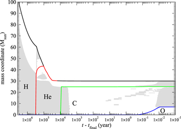
Figure 2. Similar to Figure 1, but for M = 100 M⊙.
Download figure:
Standard image High-resolution image
Figure 3. Similar to Figure 1, but for M = 120 M⊙.
Download figure:
Standard image High-resolution imageAt solar metallicity the high metal content in the initial composition has largely increased the opacity, which allows strong mass loss during H-burning and He-burning due to the star's intrinsic high luminosity. It has an extremely large mass loss rate such that half of the matter is lost in the helium-burning phase for M = 80 and 100 M⊙, and in the hydrogen-burning phase for 120 M⊙. The whole H envelope is lost during He-burning, which occurs about 105 yr before collapse. The initial He-core mass can reach about half of the initial total mass, but it gradually decreases due to the later mass loss. Also, in all three models, after the removal of the H envelope or He-burning, the C core quickly forms with a mass similar to that of the He core. Models of 80 and 100 M⊙ have a C-core mass ∼20 M⊙, which remains unchanged after it has been formed. The 120 M⊙ model has a somewhat smaller one due to the previous drastic mass loss.
The convective pattern of the star is consistent with that of a typical massive star. In the H-burning phase, the core is mostly convective while the surface is radiative. In the He-burning phase, the core remains convective while some of the H envelope becomes convective. But this feature disappears when the mass loss sheds the H envelope. Once the C core has formed at about 104 yr before pulsation, the star begins to contract rapidly. The core becomes radiative. But together with the C-core and burning of the C envelope, layers of convective shells appear. They gradually propagate and reach the surface of the C core. When the core starts O-burning (10−1 yr from the onset of first pulsation), the strong energy generation triggers large-scale convection whereby the whole C envelope becomes convective. The inner core of the O-rich region also becomes convective.
We plot Figures 4–6 similarly to the previous three figures but at Z = 0.1 Z⊙. Different from the models at solar metallicity, the low metallicity implies low opacity in the matter, which thus lowers the mass loss during the H- and He-burning phase. There is a clear signature of a massive He core from 30 to 50 M⊙. The He-core mass remains constant after it has formed. Near the occurrence of first pulsation, a massive CO core ∼10 M⊙ is also formed. A generally larger O-rich core is formed at the end of the simulation.

Figure 4. Kippenhahn diagram of the main sequence of M = 80 M⊙ at 0.1 Z⊙ from the H-burning until the core reaches a temperature of 109.4 K.
Download figure:
Standard image High-resolution image
Figure 5. Similar to Figure 4, but for M = 100 M⊙.
Download figure:
Standard image High-resolution image
Figure 6. Similar to Figure 4, but for M = 120 M⊙.
Download figure:
Standard image High-resolution imageDue to the preservation of the H envelope after He-burning, the star consists of a rich structure of convective activity before its collapse. The convective core has a similar structure to the case of higher metallicity, due to the extended H envelope that remains after He-burning. There is also a second convective zone, which gradually moves inward to the stellar core from its initial 60 M⊙ to ∼40 M⊙. Thereafter the He core is fully convective during He-burning and the convective zone extends into the H envelope. The surface is also convective. During C-burning, the convective layer propagates outward from the core to the surface of the C core. The outer layers of He and C envelopes are convective. During contraction before the onset of O-burning, the core returns to being mainly radiative. Similar to the case of high metallicity, the core becomes convective near the onset of pulsation.
3.2. Pre-pulsation Evolution
In the left panel of Figure 7 we plot the H-R diagram for the main-sequence star models with M = 80, 100, 120, and 140 M⊙ included. All models are fixed at Z = 0.002 Z⊙. For numerical stability we do not include mass loss for the 140 M⊙ model. In the pre-pulsation evolution, the models follow the typical H-R diagram of a main-sequence star. H-burning occurs after the star has contracted. After H is exhausted, the star develops into a red giant with He-burning, which greatly increases its luminosity. Depending on the mass loss, the effective temperature can reduce considerably. Also, the typical luminosity increases with mass.

Figure 7. Left: H-R diagram of the main-sequence stars from 80 to 140 M⊙. Notice that no mass loss is assumed for the 140 M⊙ model due to the later numerical instability. Right: similar to the left panel, but for Tc plotted against ρc. The zone enclosed by the purple curve corresponds to the instability zone defined by Γ < 4/3.
Download figure:
Standard image High-resolution imageIn the right panel we plot the evolution of the central temperature against the central density for the same set of models. We also draw the pair-instability zone (defined by the adiabatic index Γ < 4/3). There is no intersection among models, showing that the thermodynamic properties of the core before pulsation depend only on its mass. The contraction of the core is mostly adiabatic (with a slope −3) in the diagram.
3.3. He-core and CO-core Mass Relations
To study the effects of metallicity and rotation, we run pre-pulsation stellar evolution models for different metallicities from Z = 10−3 Z⊙ up to Z = 1 Z⊙ for a non-rotating main-sequence star. In Table 1 we tabulate the pre-pulsation configurations of the main-sequence stars for their He- and CO-core masses when the core exhausts all H and He respectively. The CO-core masses are written in brackets.
Table 1. The Pre-pulsation He-core Mass at the Exhaustion of H in the Core
| Mass (M⊙) | Z = 10−3 Z⊙a | a | ||||
|---|---|---|---|---|---|---|
| 80 | 34.05 | 37.40 (27.20) | 33.80 (23.93) | 30.10 (23.96) | 23.60 (21.09) | 22.70 (18.66) |
| 100 | 44.51 | 49.44 (37.69) | 47.16 (34.22) | 33.00 (30.65) | 31.70 (28.50) | 30.30 (24.85) |
| 120 | 54.87 | 64.71 (48.40) | 59.95 (43.48) | 57.10 (41.20) | 37.40 (31.73) | 15.50 (12.02) |
| 140 | 65.87 | nil | 70.85 (56.67) | 60.78 (50.36) | 20.80 (16.90) | 12.80 (9.60) |
| 160 | 76.50 | 83.31 (82.40) | 89.99 (89.12) | 52.93 (46.46) | 15.00 (11.63) | 11.99 (8.90) |


Notes. The numbers in brackets are the CO-core mass at the exhaustion of He in the core. All masses are in units of the solar mass.
aThe models assume no mass loss.Download table as: ASCIITypeset image
He-core mass grows monotonically with M when Z < 0.625 Z⊙. For star models with a higher metallicity, the mass loss rate, which is proportional to the metallicity, makes the He-core mass drop at the high-mass end. This transition starts at a lower mass for models with a higher metallicity. Notice that the change and the transition mass are not linearly proportional to Z due to the nonlinear dependence on mass loss rate. Also, the mass loss affects the gravity, which changes the equilibrium structure of the star even in the H-burning phase.
In Figure 8 we also plot He-core mass against progenitor mass for different metallicities. On the one hand, at low mass, the He-core mass is not so sensitive to metallicity, and it approaches its asymptotic value when Z ≤ 10−2 Z⊙. On the other hand, at high mass, the He-core mass is very sensitive to metallicity, and from Z = 0.625 Z⊙ to Z = Z⊙ it can drop by 90% for the star model with M = 160 M⊙, to about 15 M⊙. At such low mass, the He core already leaves the regime of pulsation pair-instability and evolves as a normal CCSN. Furthermore, the maximum He-core mass for models at solar metallicity only barely reaches the transition mass of 40 M⊙.

Figure 8. The He-core mass against progenitor mass when the core exhausts its hydrogen for stellar models at different metallicity. For Z = 10−2 Z⊙, the model assumes no mass loss because of numerical instability encountered during He-burning in the asymptotic red giant branch.
Download figure:
Standard image High-resolution imageFor models that completely cover the PPISN mass range (He star of mass 40–64 M⊙), we require a stellar model with a metallicity of at most 0.1 Z⊙. This shows that the PPISN is very sensitive to the progenitor metallicity, while stars with solar metallicity are less likely to form PPISNe owing to their mass loss.
Then we examine the CO-core mass. Before the CO-core mass can be defined, the massive CO core has already started its contraction, which increases its mass. The effect of metallicity is similar to the trend for He-core mass. In all models, the CO-core mass in general increases with progenitor mass at the lower-mass branch, but it drops at the high-mass end. The CO-core mass also shows a monotonic decrease with metallicity for the same progenitor mass. The effect of mass loss in models with near solar metallicity is more significant because the CO-core mass is less than 10% of the stellar mass, while in models with a lower metallicity it can be about one third of the progenitor mass.
In Figure 9 we also plot the CO-core mass against progenitor mass at different metallicities. The significance of the metallicity for the mass loss rate can be seen. As models increase from 0.5 Z⊙ to 0.75 Z⊙, the CO-core mass can drop by 75% at M = 160 M⊙. The CO-core mass shows a clearer relation than the He-core mass. The mass scales clearly with metallicity, except at M = 160 M⊙, where the model without mass loss (Z = 10−2 Z⊙) has a lower mass than its counterpart with Z = 0.1 Z⊙.

Figure 9. The CO-core mass against progenitor mass when the core exhausts its He for stellar models at different metallicities. Again, for Z = 10−2 Z⊙ the models assume no mass loss due to numerical instability.
Download figure:
Standard image High-resolution image4. PPI in Helium Stars
In this section we study the evolution of PPISNe using the zero-age He main sequence as the initial condition. We consider a stellar model with pure He, i.e., zero metallicity, because a massive He core is likely to be formed when Z ≤ 10−1 Z⊙. We do not evolve dynamically with H because the H envelope is not tightly bound by the gravitational well of the star. It is easily disturbed and obtains high velocity during shock outbreak. We find that to keep the H envelope while evolving the whole star is computationally difficult. However, as the H envelope does not couple strongly to the inner core, the pulsation dynamics is not significantly changed when we do not consider its effects. Therefore, in this section, we consider the dynamics, energetics, mass loss, and chemical properties of the PPISN by using the He star as the initial condition. However, we notice that in general an He star does not always correspond one-to-one to the He core evolved from traditional stellar evolution. We also remark that the core masses for the major elements are defined by the mass coordinate where that particular element (or major isotope) reaches a mass fraction >1%. The convective mixing is switched off when we use the hydrodynamics option because of the numerical difficulties. In fact, the dynamical timescale can be shorter than mixing timescale when the shock has formed or is dynamically expanding. It is unclear for those scenarios whether convection can be formed robustly. An incomplete mixing model or time-dependent convection model is necessary to follow this part of the input physics.
4.1. Evolution in the Kippenhahn Diagram
In this part we examine the overall evolution of the PPISN from the He core until the onset of Fe-core collapse.
In Figures 10 and 11 we plot the Kippenhahn diagrams of models He40A, He50A, He60A, and He62A. The colored zone is again the convective zone while the lines (solid, dotted, dashed, long-dashed, dotted–dashed) are the He-, C-, O-, Si-, and Fe-core mass coordinates. The x-axis is the time counting backward from the star's collapse. We define the core boundary to be the inner boundary of the mass fraction for that corresponding element to drop below 10−2. Therefore, since we start from an He core, the He-rich surface, which is also the total mass of the star, stands for the He core. Notice that for the cases with strong mass ejection, the whole He-rich surface can be shed. Here the time is defined by the time remaining until the onset of final collapse.

Figure 10. Left: Kippenhahn diagram for the model He40A (MHe = 40 M⊙) until the onset of final collapse. The lines correspond to the inner boundary where the mass fractions of the respective elements drop below 10−2. By this definition, the surface mass coordinate of the star, if it does not experience strong mass ejection, is the He-core mass since we start from an He star. Right: similar to the left panel but for MHe = 50 M⊙. The time on the x-axis is defined by the time before the onset of final collapse.
Download figure:
Standard image High-resolution image
Figure 11. Similar to Figure 10, but for MHe = 60 M⊙ (left) and MHe = 62 M⊙ (right).
Download figure:
Standard image High-resolution imageFor model He40A, after the strong pulsation, the star expands and the outer part of the star above 18 M⊙ becomes convective. Also, the star has established its O and Si cores at m(r) ∼ 5 M⊙ and its Fe core at m(r) ∼ 2 M⊙. Radiative transfer remains the major means of energy transport in the core. Thin layers of convection shells can be found in most parts of the He and C envelope. At about 10−1 yr, the Si and O core can reach as far as ∼30 M⊙. This is because during the propagation of the acoustic wave near the surface, the density gradient accelerates the wave into a shock, which heats up the matter around it. As a result, in such He-rich material, it facilitates He-burning and yields product including C, O, Ne, and Si. However, together with the extended convection during the expansion–contraction phase, the outer O- and Si-rich zones disappear and the values correspond to the inner layers, which come from previous hydrostatic burning.
For model He50A, after the pulsation, the C, O, and Si cores are produced simultaneously. But the O and Si cores quickly retreat from 30 M⊙ to 5 and 10 M⊙ respectively. The early formation of O and Si cores occurs because when the shock reaches the surface, the shock heating is capable of producing O- and Si-rich material around that region, but no significant O and Si production takes place away from the shock-heated zone. However, after its production, the mixing and mass loss caused by pulsation quickly remove this material. As a result, the O- and Si-core mass coordinates return to the corresponding inner values, where the real O and Si cores are located. At 10−3 yr before the final collapse, the contraction of the star allows the central density to be high enough for burning until NSE. The Fe and neutron-rich cores form almost simultaneously at ∼2 M⊙. Unlike model He40A, the inner core is no longer convective, except after pulsation. There is an extended period of time at ∼10−2 yr before its final collapse in which the star continues to hold fragmented convective layers.
For model He60A, there is also no inner convective core after its pulsation. Again, the shock heating creates a temporary outer surface to the O and Si cores, but they return to their inner ones after mass ejection and mixing, to ∼5 and 15 M⊙. Unlike the previous two models, the expanded star after pulsation does not reach any convective state before its second pulse or final collapse. An outward propagating convective structure can be seen from ∼1 yr before collapse. It moves from m(r) = 20 M⊙ to 40 M⊙. The convective zone is small so it does not contribute in bringing the fuel from outer layers to the actively burning layer. Similar to model He50A, the Fe and neutron-rich cores appear at ∼2 M⊙ at 10−3 yr before collapse.
Model He62A is different from the previous three models because of its extensive mass loss after pulsation. After the first pulse, the star reaches a very extended period of ∼104 yr in a fully convective state. Again, the convection washes away the external C and O envelope. The first pulse creates final C and O cores, which are located at 20 and 5 M⊙ respectively. In the second pulsation, the Fe core is also produced and has a mass ∼3 M⊙. During its contraction at 1 yr before its final collapse, the core reaches the third convective state. During contraction, the outer extended convective zone also moves outward from 20 to 40 M⊙. The convective structure is again fragmented. A 2 M⊙ Fe core is formed only near 10−3 yr before the final collapse.
4.2. Pre-pulsation Evolution
We first present the results for the pre-collapse profile based on the He main-sequence star in Table 2. The pre-pulsation evolution uses the hydrostatic approximation and it is continued until the central temperature reaches 109.4 K, where the dynamical timescale begins to be comparable with the O-burning timescale. Below 109.3 K the star evolves in a quasi-static manner but not assuming hydrostatic equilibrium. From the table we can see that the initial He-core mass affects the pre-pulsation C and O core. We choose the He-core models with a mass from 40 to 64 M⊙, which produce CO cores from 30.82 to 50.42 M⊙, with the remaining unburnt He in the envelope.
Table 2. The Main-sequence Star Models Prepared by the MESA Code
| Model | Mini | Mfin | MH | MHe | MC | MO | Remarks |
|---|---|---|---|---|---|---|---|
| He40A | 40 | 40 | 0 | 6.79 | 3.13 | 27.5 | only He core |
| He45A | 45 | 45 | 0 | 7.38 | 4.03 | 31.3 | only He core |
| He50A | 50 | 50 | 0 | 7.82 | 4.16 | 35.2 | only He core |
| He55A | 55 | 55 | 0 | 8.27 | 4.30 | 39.0 | only He core |
| He60A | 60 | 60 | 0 | 8.69 | 4.43 | 42.9 | only He core |
| He62A | 62 | 62 | 0 | 8.77 | 4.59 | 44.6 | only He core |
| He63A | 63 | 63 | 0 | 8.89 | 4.64 | 45.3 | only He core |
| He64A | 64 | 64 | 0 | 8.96 | 4.63 | 46.1 | only He core |
Note. Mini and Mfin are the initial and final masses of the star. MH, MHe, and MCO are the hydrogen, He, and CO masses before the hydrodynamics code starts. All masses are in units of solar mass.
Download table as: ASCIITypeset image
In Figure 12 we present the initial model profile and its composition. We find that most models are very similar to each other, so for demonstration we picked as an example. The star consists of three parts: a slowly varying core that extends up to 50 M⊙, an envelope of rapidly falling density, and a surface with rapidly falling temperature.


Figure 12. Left: the initial profile of density and temperature of model He60A. Right: similar to the left panel, but for the chemical composition including 4He, 12C, 16O, and 20Ne.
Download figure:
Standard image High-resolution imageIn the right panel we plot the chemical abundance profile for the same model. The model contains a flat core of mostly 16O up to ∼50 M⊙. Then it becomes C-rich and then He-rich until the surface of the star.
4.3. Pulsation
We first study the time evolution of the pulsation. To do so, we examine the second pulse of model He60A, which is a strong pulse (with mass ejection) of mass ≈ 10 M⊙. We choose this particular pulse because it is strong enough to create global change in the profile so that we can understand the changes during the contraction phase (before the maximum central temperature in the pulsation) and expansion phase (after the minimum in the pulsation).
The core is mostly supported by the radiation pressure. With the catastrophe in pair production, the supporting pressure suddenly drops, where the core softens with a corresponding adiabatic index of the equation of state of γ < 4/3 in the core. However, unlike stars with a mass of 10–80 M⊙, which have rich Fe cores at the moment of their collapse, in PPISNe and PISNe the core is mostly made of 16O when contraction starts. The softened core allows a very strong contraction and the 16O-rich core can reach the explosive temperature, which releases a large amount of energy, sufficient to disrupt the star. 28Si and 56Ni can be produced during the contraction, when the central temperature can reach above 109.5 K. As a result, the star stops its contraction and expands. The rapid expansion causes strong compression of matter on the surface, which efficiently causes ejection of high-velocity matter from the surface and dissipates the energy. After that, the core becomes bound again. The pulsation restarts after it has lost most of its previously produced energy by radiation and neutrinos. The whole process repeats until the 56Fe core, formerly 56Ni, exceeds the Chandrasekhar mass and collapses under its own gravity before the compression heating can reach the further outgoing 16O-rich envelope.
In Figure 13 we plot the temperature, density, and velocity evolution at selected times in the top left, top right, and middle left panels, respectively. We pick the profiles when the core temperature reaches 109.3, 109.4, and 109.5 K before its peak during the pulse for profiles 1–3, at its peak temperature for profile 4, and after the core has reached its peak temperature for profiles 5–7 for the same central temperature interval. We plot the chemical abundance profiles for isotopes 16O, 28Si, and 56Ni in the middle right, bottom left, and bottom right panels respectively.

Figure 13. Top left: the temperature evolution of model He60A around the second pulse. The profiles are chosen such that the central temperature reaches 109.3 K (profile 1), 109.4 K (profile 2), 109.5 K (profile 3) before the pulse, during the peak (profile 4), and the central temperature returns to 109.5 K (profile 5), 109.4 K (profile 6), and 109.3 K (profile 7). Top right: similar to the top left panel, but for the density profiles. Middle left: similar to the top left panel, but for the velocity profiles. Middle right: similar to the top left panel, but for 16O mass fraction. Bottom left: similar to the top left panel, but for 28Si mass fraction. Bottom right: similar to the top left panel, but for 56Ni mass fraction.
Download figure:
Standard image High-resolution imageFirst we study the hydrodynamics quantities. For the temperature, in the contraction (expansion) phase the star shows a global heating (cooling) due to the compression (expansion) of matter, and no temperature discontinuity can be observed. This shows that the whole star contracts adiabatically, without producing explosive burning in the star. By comparing the temperature profiles at the same central temperature (profiles 1 and 7 for Tc = 109.3 K, profiles 2 and 6 for Tc = 109.4 K, and profiles 3 and 5 for Tc = 109.5 K), the net effect of nuclear burning can be extracted. The part outside q ∼ 0.3 has a higher temperature after the pulse. A similar comparison can be carried out for the density profile. The inner core within q ∼ 0.3 is unchanged after pulsation, while the density in the outer part increases. The velocity profiles show more features during the pulse. Before the star reaches its maximally compressed state, the velocity everywhere is much less than 108 cm s−1. At the peak of the pulse, the envelope has the highest infall velocity of ∼2 × 108 cm s−1. After that, in profile 5, the core starts the homologous expansion phase, with a sharp discontinuous velocity peak near the surface between the outward-going core matter and the infalling envelope. Beyond profile 6, the discontinuity reaches the surface and creates a shock breakout. The surface matter can freely escape from the star.
For the chemical composition, the effects of the pulse become clear. By the time of the second pulse, part of the 16O core has already been consumed and converted to 28Si in the first pulse. During the compression, before the core reaches its maximum temperature, 16O is significantly consumed and forms 28Si. When the core reaches the peak temperature, the O within q ≈ 0.06 is completely burnt, which is where intermediate-mass elements, such as 28Si, are produced. However, Fe-peak elements, such as 56Ni, are not yet produced. On the other hand, during the expansion phase, most O-burning has ceased, making the 16O and 28Si unchanged after the central temperature reaches 109.4 K, while advanced burning still proceeds slowly to form Fe-peak elements.
4.4. Global Properties of a Pulse
Here we study some representative models of an He core with a mass from 40 to 62 M⊙. They show very different pulsation histories by their numbers of pulses and their corresponding strengths. In Table 3 we tabulate the stellar mass and the mass of elements in the star after each pulse.
Table 3. The Masses and Chemical Compositions of the Models
| Model | Bounce | Msum | MHe | MC | MO | MMg | MSi | MIME | MNi | MFe group | Remark |
|---|---|---|---|---|---|---|---|---|---|---|---|
| He40A | 1 | 40.00 | 6.77 | 2.65 | 26.70 | 0.69 | 0.96 | 3.89 | 0.00 | 0.00 | Weak |
| He40A | 2 | 40.00 | 6.65 | 2.34 | 24.70 | 0.81 | 1.99 | 6.30 | 0.00 | 0.01 | Weak |
| He40A | 3 | 40.00 | 6.59 | 2.14 | 23.16 | 0.89 | 2.95 | 7.70 | 0.11 | 0.40 | Weak |
| He40A | 4 | 40.00 | 6.57 | 2.07 | 22.52 | 0.91 | 3.07 | 7.83 | 0.24 | 1.01 | Weak |
| He40A | 5 | 40.00 | 6.54 | 1.94 | 21.77 | 0.92 | 3.13 | 7.79 | 0.24 | 1.91 | Weak |
| He40A | 6 | 40.00 | 6.51 | 1.85 | 20.06 | 0.92 | 3.43 | 7.78 | 1.69 | 3.76 | Strong |
| He40A | E | 37.78 | 4.68 | 1.79 | 20.06 | 0.91 | 3.43 | 7.77 | 0.07 | 3.42 | Final |
| He45A | 1 | 45.00 | 7.19 | 3.00 | 30.87 | 0.83 | 0.62 | 3.94 | 0.00 | 0.00 | Weak |
| He45A | 2 | 45.00 | 7.00 | 2.48 | 28.05 | 1.13 | 2.41 | 7.47 | 0.00 | 0.01 | Weak |
| He45A | 3 | 45.00 | 6.92 | 2.32 | 26.60 | 1.16 | 3.43 | 9.04 | 0.00 | 0.11 | Weak |
| He45A | 4 | 45.00 | 6.91 | 2.20 | 25.36 | 1.19 | 4.11 | 9.78 | 0.56 | 0.75 | Strong |
| He45A | E | 39.26 | 1.74 | 1.95 | 25.32 | 1.17 | 3.43 | 8.44 | 0.06 | 1.80 | Final |
| He50A | 1 | 50.00 | 7.59 | 2.95 | 34.61 | 1.10 | 0.84 | 4.85 | 0.00 | 0.00 | Weak |
| He50A | 2 | 50.00 | 7.38 | 2.41 | 31.16 | 1.37 | 3.13 | 9.03 | 0.02 | 0.02 | Weak |
| He50A | 3 | 50.00 | 7.29 | 2.15 | 28.38 | 1.35 | 5.06 | 11.62 | 0.47 | 0.57 | Strong |
| He50A | E | 47.39 | 5.21 | 2.17 | 28.38 | 1.33 | 4.08 | 9.80 | 0.09 | 1.73 | Final |
| He55A | 1 | 55.00 | 7.96 | 2.83 | 38.00 | 1.47 | 1.27 | 6.20 | 0.00 | 0.00 | Weak |
| He55A | 2 | 55.00 | 7.87 | 2.42 | 35.06 | 1.62 | 3.46 | 9.63 | 0.02 | 0.03 | Strong |
| He55A | 3 | 53.55 | 6.35 | 1.92 | 31.70 | 1.72 | 4.64 | 11.17 | 1.99 | 2.40 | Strong |
| He55A | E | 48.22 | 1.75 | 1.59 | 31.66 | 1.53 | 4.50 | 10.72 | 0.01 | 2.49 | Final |
| He60A | 1 | 60.00 | 8.43 | 2.75 | 41.71 | 1.72 | 1.67 | 7.11 | 0.00 | 0.00 | Strong |
| He60A | 2 | 59.52 | 7.91 | 2.22 | 36.78 | 1.64 | 5.42 | 12.46 | 0.13 | 0.15 | Strong |
| He60A | E | 51.48 | 0.75 | 1.92 | 36.75 | 1.61 | 4.21 | 10.32 | 0.09 | 1.64 | Final |
| He62A | 1 | 62.00 | 8.52 | 2.44 | 41.91 | 1.85 | 3.11 | 9.13 | 0.00 | 0.00 | Strong |
| He62A | 2 | 58.34 | 4.85 | 1.75 | 37.17 | 1.84 | 5.63 | 12.88 | 1.49 | 1.68 | Strong |
| He62A | E | 49.15 | 0.07 | 0.09 | 34.52 | 1.60 | 4.88 | 10.96 | 0.04 | 2.66 | Final |
| He64A | 1 | 64.00 | 8.69 | 2.39 | 42.87 | 1.90 | 3.63 | 10.05 | 0.00 | 0.00 | Strong |
| He64A | E | 0.00 | 0.00 | 0.00 | 0.00 | 0.00 | 0.00 | 0.00 | 0.00 | 0.00 | Final |
Note. "Bounce" means the number of the pulse in chronological order, where "E" stands for the model at the end of the simulation. Msum is the current mass in units of solar mass. MHe, MC, MO, MMg, MSi, MIME, MNi, and MFe Group are the masses of He, C, O, Mg, Si, intermediate-mass elements, Ni, and elements of nuclear statistical equilibrium in the star. For a weak pulse, the moment is defined by the minimum temperature reached between pulses. For a strong pulse, the composition is determined when the core cools down to a central temperature of 109.3 K.
Download table as: ASCIITypeset image
For model He40A, most of the pulses are weak; however, following each pulse, the mass of 16O is gradually consumed and produces 28Si. In late pulses, where the core exceeds 107 g cm−3, NSE elements are also produced. In the last pulse, the core is sufficiently compressed that an Fe core beyond 1.4 M⊙ is produced, which is followed by later mass loss. Most of the ejected mass is He.
For model He45A, most of the pulses are weak. As the number of pulses increases, not only Si but also 56Ni is produced. The last pulse, which is the strongest overall, produces about 0.56 M⊙ Ni, while the generated heat creates a shock to eject about 6 M⊙ matter before the final collapse.
For model He50A, there are fewer pulses and again only the last pulse is a strong one that can eject mass. Compared to previous models, more 16O is consumed in each pulse, which produces Si. At the final strong pulse, less Ni is produced, while the accompanying mass loss ejects the He in the envelope. It should be noted that its lower mass ejection than model He45A arises because the O in model He45A is burnt in a much compressed state. This creates a much stronger pulsation when the expansion approaches the surface, which increases the mass loss.
Model He55A has two strong pulses, in contrast to lower-mass models that have only one. Its pulses are qualitatively similar to those in model He50A.
Model He60A has no weak pulse. The contraction always causes a significant mass of O to be burnt to produce the thermal pressure to support the softened core against its contraction. Due to the strong mass ejection, at the end of the simulation the star almost runs out of He. However, one difference between this model and the others is that it has a much lower Ni mass after pulsation. Most of the Fe, which leads to the collapse, is created during the contraction toward collapse.
Model He62A has a similar pulse pattern to model He60A but is stronger. Each pulse can consume about 3−4 M⊙ of O. Unlike previous models, model He62A has an abundant amount of O even during its contraction toward collapse, and O continues to be consumed before it collapses.
Model He64A, which is a PISN instead of PPISN, has only one pulse before its total destruction. Due to its much lower density when large-scale O-burning occurs, even when about a few solar masses of O is burnt during the pulse, the energy is sufficient to eject all mass when the pulse reaches the surface.
4.5. Thermodynamics
In Figures 14–16 we plot the central density and temperature against time for models He40A, He45A, He50A, He55A, He60A, and He62A. To show that the rapid contraction comes from the PPI, we show in each plot the zones where electron–positron pair creation, the dynamical instability induced by photodisintegration of matter in NSE at Ye = 0.5 (Ohkubo et al. 2009), and the dynamical instability induced by general relativistic effects (Osaki 1966) apply. The arrows in the figures show where the pulses take place. Here we define weak and strong pulses as the pulsation of the star without and with mass ejection. The strength of the pulse is further defined by how much the core expands and cools down.

Figure 14. The central temperature against central density for model He40A (top) and model He45A (bottom). In each plot, the region on the left of the blue line represents regimes dominated by the dynamical instability of pair creation, general relativistic effects (see, e.g., Osaki 1966) and photodisintegration of matter in NSE at Ye = 0.5 (Ohkubo et al. 2009). The arrows indicate where the pulsations take place.
Download figure:
Standard image High-resolution image
Figure 15. The central temperature against central density for model He50A (top) and model He55A (bottom). The blue lines and the arrows have the same meaning as in Figure 14.
Download figure:
Standard image High-resolution image
Figure 16. The central temperature against central density for model He60A (top) and model He62A (bottom). The blue lines and the arrows have the same meaning as in Figure 14.
Download figure:
Standard image High-resolution imageFor model He40A, at the beginning the central density is the highest among all six models. It thus has weaker pulses because the core is more compact and degenerate. It has five weak pulses and one strong pulse (indicated by arrows in the figure) where each of the small pulses only leads to a small drop in the central density and temperature. Then the core quickly resumes its contraction again. Only at the final pulse, when the core begins to reach the Fe photodisintegration zone, does the softened core lead to a fast contraction and reach a central temperature Tc = 109.8 K. This triggers large-scale O-burning in the outer core, which leads to a drastic drop in the central density and temperature, showing that the star is expanding, until Tc reaches 109.2 K. Then the core resumes its contraction. Since most O in the core is burnt, the Si-burning cannot produce adequate energy to create further pulsations. The star directly collapses.
Model He45A shows fewer pulses than model He40A. It has three weak pulses and one strong pulse. The initial path is closer to the PC instability zone. The last pulse is triggered at Tc = 109.7 K and has the lowest Tc of 108.9 K when it is fully expanded.
Model He50A has only two weak pulses and one strong pulse. Its evolution shows less structure than the previous two models because of the earlier trigger of large-scale O-burning in the core. The core starts the big pulse when Tc = 109.6 K and its expansion causes Tc to reach 108.8 K at minimum. Before its collapse, there is a small wiggle along its trajectory. We notice that in this phase the core has a small pulsation when it core becomes degenerate.
Model He55A has one weak pulse and two strong pulses. The two strong pulses start when Tc reaches 109.5 and 109.7 K respectively, with a minimum temperature after relaxation at 108.8 and 108.6 K.
For model He60A, there is no weak pulse and two strong pulses, where the stellar core intersects with the PC instability zone during its expansion. The two pulses start when Tc reaches 109.4 and 109.6 K. The core finishes its expansion when it reaches 109.0 and 108.3 K.
For model He62A, the star model becomes very close to the PC instability where the core enters the zone for a short period of time during its expansion. It is similar to model He60A in that there are two strong pulses. The two peaks start at 109.5 and 109.7 K and both pulses end at a minimum temperature of 108.4 K, showing that the two pulses are of similar strength. After that, the core starts collapsing similarly to the other five models.
By comparing all six models, we can observe the following trend for the pulse structure as a function of progenitor mass. First, when the progenitor mass increases, the number of small pulses decreases while the number of big pulses increases. Second, the strength of the big pulses increases with progenitor mass, which leads to a lower central temperature and density during its expansion. Third, the path during its early pulses becomes closer to the PC instability as mass increases. Fourth, the second strong pulse is stronger than the first.
4.6. Energetics
In Figures 17–19 we plot the energy evolution for models He40A, He45A, He50A, He55A, He60A, and He62A, including the total energy Etotal, internal energy Eint, gravitational energy Egrav, and kinetic energy Ekin. The energy is scaled in order to make the comparison easier.

Figure 17. Total Etotal, internal Eint, net gravitational Egrav, and kinetic Ekin energies against time for models He40A (left) and He45A (right).
Download figure:
Standard image High-resolution image
Figure 18. Similar to Figure 17, but for models He50A (left) and He55A (right) .
Download figure:
Standard image High-resolution image
Figure 19. Similar to Figure 17 but for models He60A (left) and He62A (right) .
Download figure:
Standard image High-resolution imageIn all six models, the energy evolution does not depend on the stellar mass strongly, except for the energy scale. In all these models, the small pulses do not make observable changes in the energy except for very small wiggles. The contraction before a pulse leads to a denser and hotter core, where neutrino emission continuously draws energy from the system. At a big pulse, the total energy shows a rapid jump, which increases close to zero, then the ejection of mass quickly removes the generated energy, making the star bound again. Similar jumps in Eint and Egrav show that the core is strongly heated due to contraction heating and nuclear reactions. After that, the star reaches a quiescent state with a mild increase in total energy due to the 56Ni decay, followed by a quick drop when it contracts again.
4.7. Luminosity
In Figures 20–22 we plot the luminosity evolution for the six models similar to Figure 17. During the pulse, the extra energy from nuclear reactions allows the luminosity to grow by 3–4 orders of magnitude. For a short period of time (≤10−2 yr), the star becomes dim suddenly. After that the star resumes its original luminosity quickly and remains unchanged until the next pulse or final collapse. We recall that the luminosity during shock breakout and shortly thereafter cannot be trusted because it requires in general non-equilibrium radiative transfer for an accurate treatment.

Figure 20. Total luminosity and neutrino luminosity against time for models He40A (left) and He45A (right).
Download figure:
Standard image High-resolution image
Figure 21. Similar to Figure 20, but for models He50A (left) and He55A (right).
Download figure:
Standard image High-resolution image
Figure 22. Similar to Figure 20, but for models He60A (left) and He62A (right).
Download figure:
Standard image High-resolution imageThe neutrino luminosity is more sensitive to the structure of the star. The neutrino luminosity can also jump by 3–10 orders of magnitude from its typical value in the hydrostatic phase to the maximally compressed state. After the star has relaxed, the neutrino luminosity drops drastically. Depending on the strength of the pulse, neutrino cooling can become unimportant in the quiescent phase.
4.8. Mass Loss History
During the pulsation, when the bounce leads to explosive burning in the core and inner envelope, sufficient energy is produced to create an outgoing shock, where the outermost matter can gain sufficient energy to be ejected from the star. The ejected matter later cools down and becomes circumstellar matter (CSM). The existence of such H-free CSM is necessary in the circumstellar interaction models for Type I superluminous supernovae (SLSNe-I) (Sorokina et al. 2016; Tolstov et al. 2017). The chemical and hydrodynamic properties of the CSM thus become important, which influences the formation of the light curve of the explosion.
In Table 4, we tabulate the mass loss history of each model and its chemical composition. In Figures 23–26 we also plot the ejecta profiles of a representative pulsation taken from models He40A, He50A, He60A, and He62A respectively. Three patterns can be observed in the mass ejection. We choose these models because these examples characterize the typical ejecta features of strong pulses in the lower and higher mass regimes. We take the numerical values when the mass shells are ejected during the pulsation because that is the last moment at which the code keeps track of their evolution.

Figure 23. The mass ejection history of model He40A. Top: ejecta density; middle: ejecta velocity and escape velocity; bottom: ejecta chemical composition.
Download figure:
Standard image High-resolution image
Figure 24. The mass ejection history of model He50A. Top: density; middle: velocity; bottom: chemical composition. For the velocity plot, the black triangles and red inverted triangles correspond to the ejecta and escape velocities at the surface.
Download figure:
Standard image High-resolution image
Figure 25. The mass ejection history of model He60A. Top: density; middle: velocity; bottom: chemical composition.
Download figure:
Standard image High-resolution image
Figure 26. The mass loss history of the second strong pulse in model He62A.
Download figure:
Standard image High-resolution imageThe first group is the strong pulse in the lower-mass branch. In models He40A and He45A the last pulse is the one that ejects mass. It displays wiggles in its density profiles, showing that the thermal expansion creates the first wave of mass ejection, followed by the shock as the velocity discontinuity approaches the surface, which creates the second wave of mass ejection. In both cases, only the He layer is affected, but as the He layer becomes thin, matter near the CO layer is ejected.
The second group is the weaker pulse of the more massive branch. In models He50A, He55A, He60A, and He62A the first strong pulse occurs after the core starts to consume O collectively. Since it burns much less O than other strong pulses, the ejection comes from the rapid expansion of the star, which includes matter in the He envelope.
The third group is the strong pulse of the more massive branch. In models He55A and He60A, the second pulse is stronger so the ejecta density gradually decreases. A continuous ejection of mass in terms of a smooth density profile is found. The mass ejection is sufficiently deep that, at the end of pulsation, traces of 12C and 16O can be found. We remark that the inclusion of massive elements (compared with H and He) will be important for future light-curve modeling because they contribute as the main source of opacity.
One of the pulsations needs to be discussed separately because of its very massive mass ejection, which involves a unique chemical composition in its ejecta. In model He62A (right plot), the second pulse becomes strong enough that, besides its decreasing density profile, the later ejected material contains a significant amount of heavier elements including C, O, Mg, and Si, showing that the He envelope is completely exhausted before the star is sufficiently relaxed.
4.9. Chemical Properties
In Figures 27–30 we plot the isotope profiles at different moments of models He40A, He50A, and He62A. We selected moments before and after each strong pulse to extract the nuclear burning history. The models are chosen to demonstrate how different strengths of pulsation and the convective mixing between pulses can create distinctive isotope abundances in the star. By comparing the isotope distribution, we can understand which part of burning contributes to the evolution of pulsation.

Figure 27. The chemical composition of model He40A before the first pulse, after the first pulse, and before the final pulse in the upper, middle, and lower plots. Here we define the star as entering the pulsation phase when the core reaches 109.3 K.
Download figure:
Standard image High-resolution image
Figure 28. Similar to Figure 27, but for model He50A before the first pulse, after the first pulse, and before the final pulse in the upper, middle, and lower plots.
Download figure:
Standard image High-resolution image
Figure 29. The abundance patterns for model He62A before the first pulse, after the first pulse, and before the second pulse.
Download figure:
Standard image High-resolution image
Figure 30. Similar to Figure 29, but for model He62A after the second pulse, before the final pulse, and at the end of simulation.
Download figure:
Standard image High-resolution imageIn all models, it can be seen that the star is simply a pure O core with a minute amount of Si in the core or C in the envelope, covered by a pure He surface. However, their changes can be very different depending on the progenitor mass.
In model He40A, after the strong pulse, a range of elements are produced due to its previous weak pulses, which continue to burn matter in the core; these include 52Fe, 54Fe, 56Fe, and also 56Ni. There is a clear structure for each layer, which follows the order of 56Fe, 54Fe, 56Ni, 40Ca, 16O, and then 4He. After that, the core relaxes and becomes quiescent until it completely loses its thermal energy produced during the pulse, while at the same time convection redistributes the matter for a flat composition profile. Most convection occurs at q > 0.1, where the convective shells of different sizes make a staircase-like structure.
Models He45A and He50A share a similar nuclear reaction pattern. We choose model He50A as an example. The strong pulse provides the required temperature and density to make Ni in the center and Si in the outer zone. The Si-rich zone extends to q ≈ 0.2. During the quiescent phase, convection mixes the material not only in the envelope but also in the core, which is seen in the stepwise distribution of 52Fe and 54Fe.
Models He55A, He60A, and He62A also share a similar abundance pattern. We choose the evolution of He62A as an example. The first pulse makes the original O core into mostly Si and some Ca. Again, the convective mixing during the quiescent state redistributes the matter near the surface (q > 0.25). In the second strong pulse, the nuclear reaction is very similar to the late pulses of models He40A and He45A. Ni forms in the innermost part, with a small amount of Fe isotopes such as 52Fe and 54Fe. Then Si and Ca form the middle layer and finally the He envelope appears. During the quiescent phase, the convection occurs in a deeper layer that is absent in lower-mass models.
5. Models for SLSNe
PPISNe have been used to model superluminous supernovae such as SN2006gy (Woosley et al. 2007), SN2010gx, PTF09cnd (Sorokina et al. 2016), and PTF12dam (Tolstov et al. 2017). PTF09cnd and PTF12dam are challenging because they require a CSM as massive as 20–40 M⊙ prior to the supernova explosion. Furthermore, these SLSNe are of Type I, so the CSM needs to be H-free with the presence of He, C, and O in order to explain the high surrounding opacity.
A model with ∼64 M⊙ He core is likely to eject a mass ∼22 M⊙. Our model gives an ejecta with He, C, and O masses of 8.5, 1.8, and 9.9 M⊙. The corresponding ratio of He:C:O is therefore 4.8:1:5.5. This is close to the values in the model M66R170E27(CSM19) of Tolstov et al. (2017), which has an abundance ratio of C:O = 1:4. Whether the subsequent collapse of this ∼40 M⊙ remnant can explode energetically with an energy of (2−3) × 1052 erg is uncertain.
In Figure 31 we plot the density profile of model He50A at the onset of collapse (ρc = 1010 g cm−3). Both the CSM and core are included. The CSM is constructed from the mass ejection history, which is obtained in a post-process manner until the core begins to collapse. The core is a compact Fe core of ∼2 M⊙ with r < 108 cm. Outside the Fe core, a smooth Si-rich envelope extends up to M(r) ∼ 10 M⊙ and r ∼ 1010 cm. The outer surface extends to ∼1012 cm. We remark that the outermost envelope is mostly the remaining matter that is not ejected near the end of the pulsation event. It is mostly decoupled gravitationally from the core. The original stellar envelope is the middle envelope of the final density profile.

Figure 31. The final density profile for model He50A including the core and ejecta matter (CSM) at the onset of collapse.
Download figure:
Standard image High-resolution imageAs discussed in Section 4.8, the mass ejection of He50A is smooth and occurs for 0.0002 yr (∼2 hr) before the outermost shell is bound. Such continuous mass ejection can produce a smooth and extended CSM outside the star. There is no significant collision among ejected masses, where a collision could give rise to observable density discontinuities. Without mass collision, the CSM profile in general follows the 1/r2 scaling, which extends from 1014 to 1016 cm. We note that in the calculation, there is a gap between the outer envelope of the core and the inner boundary of the CSM from 1011 to 1014 cm. There should be fallback caused by gravitational tidal force on the ejecta. However, to resolve this, one requires another hydrodynamical experiment to follow how the ejecta exchanges momentum.
Table 4. Energetic and Chemical Composition of the Ejecta
| Model | Pulse | Time | Mej | Eej | Tej | M(He) | M(C) | M(O) | M(Ne) | M(Mg) | M(Si) |
|---|---|---|---|---|---|---|---|---|---|---|---|
| He40A | 6 | 9.9 × 10⁻² | 1.0 | 1.0 | 6.3–6.8 | 1.0 | 0.0 | 0.0 | 0.0 | 0.0 | 0.0 |
| He45A | 1 | 7.4 × 10⁻² | 4.0 | 6.6 | 6.5–6.9 | 3.8 | 0.2 | 0.0 | 0.0 | 0.0 | 0.0 |
| He50A | 2 | 2.0 × 10⁻¹ | 4.0 | 2.5 | 6.7–7.2 | 3.9 | 0.1 | 0.0 | 0.0 | 0.0 | 0.0 |
| He55A | 1 | 6.2 × 10⁻² | 0.3 | 1.8 | 6.8–7.1 | 0.3 | 0.0 | 0.0 | 0.0 | 0.0 | 0.0 |
| He55A | 2 | 1.9 | 10.0 | 13.1 | 6.0–6.7 | 7.5 | 1.0 | 0.8 | 0.2 | 0.3 | 0.2 |
| He60A | 1 | 1.7 × 10⁻¹ | 10.6 | 5.1 | 5.3–6.4 | 8.6 | 2.4 | 0.8 | 0.6 | 0.2 | 0.2 |
| He60A | 2 | 7.4 × 10³ | 38.7 | 59.0 | 6.0–6.5 | 0.0 | 1.1 | 32.5 | 1.3 | 1.3 | 2.0 |
| He62A | 1 | 5.5 × 10⁻² | 0.6 | 0.1 | 6.8–7.4 | 0.6 | 0.0 | 0.0 | 0.0 | 0.0 | 0.0 |
| He62A | 1 | 3.5 × 10³ | 55.4 | 29.6 | 4.6–7.2 | 7.8 | 1.7 | 33.2 | 1.6 | 1.8 | 5.8 |
| He64A | 1 | 4.9 × 10⁻² | 21.8 | 29.4 | 4.4–7.1 | 8.5 | 1.8 | 9.9 | 0.9 | 0.3 | 0.6 |
Note. "Pulse" stands for the sequence of pulses in its evolution. "Time" is the occurrence time in units of year. Tej is temperature range of the ejecta in units of K. Eej is the ejecta energy in units of 1050 erg. M(He), M(C), M(O), M(Ne), M(Mg), and M(Si) are the masses of He, C, O, Ne, Mg, and Si in the ejecta in units of solar mass.
Download table as: ASCIITypeset image
6. BH Masses from Pulsational PISNe
The GW detectors aLIGO and VIRGO have recently detected GW signals from merger events of compact objects. Some massive BHs are measured, for example BH masses of 35.6+4.6–3.0 and 30.6+3.0–4.4 M⊙ in GW150914 (Abbott et al. 2016b). Another massive BH merger event is GW170104, where the binary consists of BHs of masses 31.0 and 20.1 M⊙. In Table 5 we list the recent GW events with BH masses reaching above 30 M⊙ within 1σ. Recent statistics have further pushed the maximum pre-merger BH mass to ∼55 M⊙ (The LIGO Scientific Collaboration et al. 2019). It is unclear whether the massive BH forms directly from the collapse of a massive star or has experienced multiple merger events prior to the event detected by the GW detectors.
Table 5. Primary and Secondary Black Hole Masses when One or Both Exceeds 30 M⊙ within 1σ
| Event | m1 | m2 |
|---|---|---|
| GW150914 | ||
| GW151012 | ||
| GW170104 | ||
| GW170729 | ||
| GW170809 | ||
| GW170814 | ||
| GW170818 | ||
| GW170823 |


Note. Events in bold font are those with black hole masses exceeding 40 M⊙. m1 and m2 are the black hole masses in units of M⊙. The data are taken from The LIGO Scientific Collaboration et al. (2019).
Download table as: ASCIITypeset image
Our model suggests that the single-star scenario has an upper limit for the BH mass. For an He core with a mass greater than 64 M⊙, the star does not collapse but explodes as a pair-instability supernova. The collapse only reappears for a star with a mass larger than 260 M⊙ (for zero metallicity) (Heger & Woosley 2002). The corresponding BH mass is .

To connect PPISNe with the measured BH mass spectra, we plot in Figure 32 the remnant mass against progenitor mass, and the mass range of the BH measured by the GW signals. For He cores with a mass between 40 and 64 M⊙, a mass correction is included to account for the pulsation-induced mass loss. Beyond the star enters the pair-instability regime and no compact remnant object is left. Near the remnant mass is the maximum at . Some of the events can be explained by the current PPISN picture. These include the primary BH in the events GW150914, GW170104, GW170729, GW170809, GW170818, and GW170823 and the secondary BH in the event GW170729.


Figure 32. The pre-collapse mass of the PPISNe against progenitor mass with the measured black hole masses obtained from binary black hole merger events (Abbott et al. 2016a, 2016b, 2017; The LIGO Scientific Collaboration et al. 2019). The left and right data points correspond to the primary and secondary black holes respectively. The error bars for the pre-merger neutron star for GW170817 are too small to be seen on the current scale.
Download figure:
Standard image High-resolution imageWe remark that there is great uncertainty in how to connect the mass of the He-core mass with that of the final remnant. In our simulations, the pulsation-induced mass loss is calculated in one dimension. When multi-dimensional effects, e.g., Rayleigh–Taylor instabilities, are considered during the propagation of a pulse, the actual mass loss can be changed. Also, after the Fe core collapses, during formation of the proto-neutron star and BH, the mass ejection and neutrino energy may reduce the final remnant mass by ∼10% (see, e.g., Zhang et al. 2008; Chan et al. 2018). We remark that interpreting the He-core mass as the final remnant mass can only be an upper limit on the BH mass. The accretion disk around a rotating BH allows the formation of a high-velocity jet. The magnetohydrodynamical instability of the accretion disk can easily fragment the disk and send the energetic jet to the stellar envelope. This process can lower the remnant mass. Therefore, as a first estimation of our result, we use the He-core mass as an upper estimate of the final BH mass.
We note that in a single observation, the solution for matching the BH mass with our remnant mass is degenerate for both mass and metallicity. To further apply the BH information in PPISNe to constrain the mass loss, the population of BH mass will become important, which can directly constrain the current mass loss model when combined with suitable stellar initial mass functions.
In Figure 33 we plot the final stellar mass, and C- and O-core masses for all the He-core models. We define the boundary of the C and O cores to be the inner boundaries where the local 4He and 12C mass fractions drop below 10−2. We can see that three layers appear. For , 45, and 50 M⊙, there are an explicit He envelope and C and O layers. For and 60 M⊙, the huge mass loss completely ejects the pure He layer, which exposes the C-rich layer (combined with He). At , the mass ejection further sheds the C-rich layer, exposing the O layer. The whole star has a mass fraction of 12C below 10−2 everywhere. Therefore, the He-core and C-core masses coincide with the total stellar mass. From this we can see the level to which mass ejection takes place for the PPISN models. However, the definition of He- and C-core masses can be ambiguous at the end of simulations because the matter becomes O-rich before C is exhausted. Similarly on the surface there can be a non-zero abundance of 12C instead of pure 4He.


Figure 33. The pre-collapse mass of the PPISN and C- and O-core masses against progenitor He-core mass. Here we define the C and O cores to be the inner boundaries where the local 4He and 12C mass fractions drop below 10−2.
Download figure:
Standard image High-resolution image7. Conclusions
In this paper, we studied PPI, which occurs in He cores of . These are the cores of 80–140 M⊙ main-sequence stars. We used the one-dimensional stellar evolution code MESA and applied the implicit hydrodynamics module implemented in the version 8118.

(1) First, we computed the evolution of stars with initial masses of 80–140 M⊙ and metallicities of Z = 0.01−1 Z⊙ from the pre-main sequence until the central temperature reaches 109.3 K. We examined how the final He- and CO-core mass depends on the metallicity. The star with a higher metallicity has a stronger mass loss by stellar wind, thus forming an He core of smaller mass. In order for the star to form an He core more massive than 40 M⊙ and thus to undergo PPI, Z ≲ 0.5 Z⊙ is required.
(2) We calculated the evolution of the He cores of with Z = 0 from the He main sequence through the onset of collapse. These He cores undergo PPI. We calculated the hydrodynamical evolution of PPI with mass ejection. We examined nucleosynthesis during PPI, showing how each pulsation changes the chemical composition of the star and how the later convection alters the post-pulsation star.

(3) The total ejected mass is almost a monotonically increasing function of MHe except for some fluctuations at the lower-mass end. The He core with a higher mass has fewer weak pulses that do not eject mass. Instead it has much stronger pulses that do eject mass. The number of pulses ranges from six weak pulses for MHe = 40 M⊙ to no weak pulse but two strong pulses for MHe = 62 M⊙. The ejecta mass is less than at the low-mass end and increases to as large as ∼10 M⊙ near the PISN regime. Models with MHe > 64 M⊙ behave as pair-instability supernovae, where no remnant is left.

(4) The ejecta form CSM. The composition and kinematics of the ejecta are sensitive to MHe. The lower-mass He cores with MHe ≲ 55 M⊙ eject only the He envelope. More massive cores eject a part of the CO layer. The most massive core studied with MHe = 62 M⊙ ejects even the Si layer. Such heavy elements may greatly alter the opacity of the CSM.
(5) We examined the connections of PPISNe, especially the ones with massive mass ejection, with the recently observed Type I superluminous supernova (SLSN-I) PTF12dam. We show that the PPISN model produces massive enough CSM, which may be able to explain some SLSNe (including PTF12dam), based on the CSM interaction. The amount of C and O is consistent with the light-curve models of SLSNe-I.
(6) We compare the masses of BHs detected from GW signals with the BH masses after the mass ejection of PPISNe. Our PPI models predict that the expected BH masses are ∼38−52 M⊙, i.e., the upper limit of the BH mass is 52 M⊙. This is consistent with current observations. Some of the events, especially GW170729 which shows a progenitor mass of ∼50 M⊙, could be a remnant left behind by a PPISN. The upper limit of the BH mass can form the lower limit of the mass gap of massive BHs (i.e., the transition from BH to no-remnant). Future observations of the BH mass spectrum derived from the merger events of binary BHs can provide the corresponding constraints on such a mass limit. The detection of BH mass prior to the merger event between ∼50 and ∼150 M⊙ can challenge the current BH formation mechanism and its progenitor evolution, and provide insight into the implied merging event rate of massive BHs evolved from PPISNe.
(7) In future work, we will focus on the observables of PPISNe in terms of neutrinos and light curves. Using our hydrodynamics model, the expected neutrino signals detected terrestrially and the expected light curve will be calculated. The results will provide a more fundamental understanding of the properties of PPISNe, which may be constrained from the observables of one of the PPISN candidates.
(8) In the appendix we show that our results are qualitatively consistent with the results in the literature, although some minor differences can be found.
This work has been supported by the World Premier International Research Center Initiative (WPI Initiative), MEXT, Japan, and JSPS KAKENHI grant No. JP17K05382. S.B.'s work on PPISNe is supported by the Russian Science Foundation Grant 19-12-00229. We thank the developers of the stellar evolution code MESA for making the code open-source. We also thank Raphael Hirschi for insightful discussion on the stellar evolution of PPISNe and his critical comments. We finally thank Ming-Chung Chu for his assistance in editing the manuscript.
Software: MESA (v8118; Paxton et al. 2011, 2013, 2015, 2017).
Appendix A: Comparison with Models in the Literature
A.1. Yoshida et al. (2016)
In this section we compare our results with some representative PPISN models in the literature.
In Yoshida et al. (2016), the PPISN models of mass from about 54 M⊙ to 60 M⊙ (corresponding to a progenitor mass from 140 M⊙ to 250 M⊙ with zero metallicity) are computed. In that work, the calculation is separated into two parts. During the quiescent and pre-pulsation phases, the hydrostatic stellar evolution code is used. During the pulsation phase, the star model is transferred to the dynamical code PPM, which follows the expansion of the star until the mass ejection has ended (∼104 s). Then they map the results to the stellar evolution code again until the next pulsation.
Their 140 M⊙ and 250 M⊙ models have similar configurations to our models He55A and He60A. First, in their 140 M⊙ model (250 M⊙ model), they observe a total of six (three) pulses, which ejected 3.99 (7.87) M⊙ of matter before collapse. Model He55A (He60A) exhibits three (two) pulses before collapse, which eject 6.78 (8.52) M⊙ of matter. Our models show a smaller number of pulses, but give similar ejecta mass. This means that our models can capture the energetic pulse well, but not the smaller pulses.
Then we compare the ejection timescales. The 140 M⊙ (250 M⊙) model shows all pulses within a period of 0.92 (1434) yr, while model He55A (He60A) shows all pulses within a period of 1341 (2806) yr. There is a huge difference in the pulsation period in our model He55A and their 140 M⊙ model. We notice that the difference comes from the strengths of the pulses. In particular, our second pulse leads to a transition at about 100 yr while ejecting 1.45 M⊙. The most similar event in their model is the fourth pulse, but with a transition of only 0.279 yr.
At last we compare the final core composition. The 140 M⊙ (250 M⊙) model has an Fe (CO) core mass of 2.57 (43.51) M⊙, while in our model, we have 2.49 (38.60) M⊙ for the Fe (CO) mass. This shows that, despite the difference in the mass ejection history, our models can still capture the major mass ejection events, which results in a similar mass ejection and core composition. However, there is a strong pulse in our He55A model that is not seen in their 140 M⊙ model.
A.2. Woosley (2017, 2019)
Next, we compare our models with the models from Woosley (2017). We have chosen the PPISN close to that work; in particular, our models He40A, He50A, He60A, and He62A can be compared directly with the He40, He50, He60, and He62 models. In Woosley (2017), the Kepler code, which consists of both hydrostatic and hydrodynamic components, is used to follow the whole evolution of PPISN.
First we compare the mass ejection history. In Woosley (2017), there are 9, 6, 3, and 7 pulses with a total mass loss of 0.97, 6.31, 12.02, and 27.82 M⊙ for models He40, He50, He60, and He62 respectively. In our models, we have 6, 3, 2, and 2 pulses with a total mass loss of 2.22, 2.61, 9.52, and 12.85 M⊙ for models He40A, He50A, He60Am and He62A respectively. Again, our code tends to produce fewer pulses and the pulses in general eject less matter. One of the differences is how shock is treated. For a shock-capturing scheme with a larger dissipation, the kinetic energy will be partly dissipated into thermal energy, such that the star is globally thermalized instead of ejecting matter through kinetic pulses. Another origin of the differences can be related to the nature of the instability of PPISNe. The trigger of the explosive O-burning comes from the pair-instability, which is very sensitive to the initial condition (e.g., how we evolve the stellar evolution model before the pulsation and between pulses) and numerical treatment (e.g., how convection and mass ejection are treated). For example, a stronger contraction can lead to more O-burning in the core, which gives much stronger pulsation and hence more mass loss. In fact, such a dependence can also be seen in other fields: for example, in the propagation of flame, since it is unstable toward hydrodynamic instability (Glazyrin et al. 2013). The burning history can be highly irregular in the unstable regime.
Next we compare the timescale of the pulsation. In this work, the whole pulsation until collapse lasts for 0.38, 61.3, 2806, and 6610 yr for the four models, while in Woosley (2017) the durations are 2.48 × 10⁻³, 0.38, 2695, and 6976 yr. This shows that our results agree with their work for massive He cores, but there are large differences when the He core becomes less massive. In that case, our final pulse is always strong enough to re-expand the star again before the final collapse, which significantly lengthens the pulsation period.
Then we compare the Fe-core mass. In Woosley (2017) the core has 2.92, 2.76, 1.85, and 3.19 M⊙ Fe. In our models, we have 3.42, 1.73, 1.64, and 2.66 M⊙. There is a decreasing trend from model He40A to He60A, which corresponds to the trend that the pair-instability occurs at a lower density when the mass increases. On the other hand, near the pair-instability regime, the pulsation becomes sufficiently vigorous to enhance the burning in NSE.
Finally we compare the explosion energy. We compare model He62A, which has the largest explosion energy. In our model, the star has its total energy increased in the second big pulse by 2.0 × 1051 erg, while the maximum kinetic energy achieved is 2.8 × 1051 erg. This is very similar to the result in Woosley (2017), where the pulse is observed to have a kinetic energy of 2.8 × 1051 erg.
One major difference we notice is in the pair-instability limit: our model He64A shows a higher explosion energy. Across the strongest pulse, there is a change in total energy by 1.6 × 1052 erg, where the maximum kinetic energy of the system is ∼1.7 × 1052 erg. In Woosley (2017) the kinetic energy is reported to be 4 × 1051 erg. We observe that the difference comes from the number of pulsations, where our model He64A has two big pulses but there is only one in their work. The first pulse has incinerated the 16O in the core while ejecting mass from the surface. This means that the star has to reach a more compact state before it can explode. As a result, the amount of energy produced in the exploding pulse is much larger.
Our results show a systematically smaller number of pulses with slightly lower ejecta mass. The pulsation periods qualitatively agree with each other except for models with a final strong pulse, which may significantly lengthen our pulsation period. Also, in our explosion models, the system tends to store the energy in terms of internal energy instead of kinetic energy; as a result, the star tends to expand globally, where the excess energy and momentum of the star are transferred mostly to the surface. This ejects the low-density matter and leaves a bound and hot massive remnant. Despite the differences in the pulsation, globally the nucleosynthesis agrees in the two models because most of the heavy elements are produced by the strong pulses, where our results are consistent with those in the literature.
In Woosley (2019), the He star models are further evolved with mass loss. The solar metallicity of the Fe group is assumed in the mass loss rate for He stars. We note that this is not consistent with the mass loss history from the main sequence, because the He core of a star of solar metallicity becomes too small to undergo PPI (see our Figure 8). The final BH mass is lower than in his previous work. We notice that the PPISN models in this work have stronger pulsations in general. A 50 (60) M⊙ He core ejects ∼7 (57) M⊙, which is much higher than ∼6 (12) M⊙ mass ejection in his previous work. Our results are closer to his previous work. This might depend on the thickness of the He layer, which is determined by the mass loss history.
A.3. Marchant et al. (2019)
This is a recent work that uses the same MESA code (Version 11123) (Paxton et al. 2017) to evolve the evolutionary path of PPISN. Their work has a similar setting to this work. Here we briefly compare their results with ours.
They have computed an array of single-star models from 40 to 240 M⊙ with semi-convection, Riemann solver using the HLLC solver, and the approx21 nuclear reaction network. They treat the mass loss of the star by considering the average escape velocity.
Our work agrees qualitatively with theirs. For a model with a lower-mass He core, some distinctive differences can be seen. For example, multiple pulsations are observed in their models. They observe a total of four pulses for the 54 M⊙ stars (corresponding to 39.73 M⊙ at He depletion). On the other hand, our model with a 40 M⊙ He star gives a total of six pulses. They observe in total 0.63 M⊙ mass ejection before collapse while ours is about 2.2 M⊙. The duration in their model is shorter (∼7 × 10⁻⁴ yr) but ours is longer (∼0.02 yr) after the onset of pulsation. For a model with a higher-mass He core such as ∼87 M⊙ (corresponding to 60.04 M⊙ at He depletion), they show only two pulses, which is the same as for our model of a 60 M⊙ He star. The duration also agrees in the two models (theirs shows a duration of 7.5 × 10³ yr while ours is shorter at 3 × 10³ yr. A total of 4.6 M⊙ mass loss is found in their model (the pre-He depletion mass loss is excluded) while ours is a higher value of ∼8.5 M⊙.
We notice that their models and our models do not completely agree with each other. We notice that there are some critical differences in the implementation of this work from their work. First, they consider the evolution of H-free stars, with a metallicity at 0.1 Z⊙. The He-core mass is therefore a function of the progenitor mass instead of a direct model parameter as controlled in our models. Furthermore, they use the Riemann solver (HLLC) in the newer version instead of the artificial viscosity scheme. How the pulse transfers into shock at the near-surface area can be different.
Appendix B: Effects of Hydrostatic Convective Mixing
In Woosley (2017) the PPISN is prepared for models with convective mixing. It is mentioned that convective mixing is essential to evolve the star correctly to readjust the chemical composition of the remnant. It is unclear how much the convective mixing can change the evolutionary path of the PPISN. Here we compare model He60A by treating the convective mixing as an adjustable parameter. In Figure 34 we plot the central temperature (upper panel) and central density (lower panel) against time for model He60A for both choices. It can be seen that the effects of convective mixing are huge. In the model with mixing switched on, in the second pulse it leads to a large amplitude expansion, which leads to significant mass loss afterwards before its third contraction to its collapse. On the other hand, the model without convective mixing has a faster growth of central temperature and central density, where the star collapses without any pulsation.

Figure 34. The central temperature (top) and central density (bottom) against time for model He60A with and without convection.
Download figure:
Standard image High-resolution imageTo understand the difference, we plot in Figure 35 the chemical composition of the star before the second contraction takes place. We pick both models for the star when it has a central temperature of 109 K. It can be seen that the role of convective mixing is clear: not only does it redistribute the energy of the matter, it also modifies the composition on the large scale. A considerable amount of fuel is re-inserted into the core, which contains O and Si from the unburnt envelope and some remaining 54Fe and 56Fe produced in the first contraction. This shows that the convection during the expansion is important for the future nuclear burning to correctly predict the strength of the pulse, which affects the nucleosynthesis as well as the mass loss.

Figure 35. The chemical abundance profiles for model He60A prior to its second contraction at a central temperature ≈109 K with convection (top) and without convection (bottom).
Download figure:
Standard image High-resolution imageTo further demonstrate the importance of convective mixing to the strength and number of pulsations, we perform a contrasting study of two models, one is model He60A and the other is similar to He60A but with enhanced mixing. We have shown in Section 4 from the Kippenhahn diagram that the convective mixing in model He60A is less strong that during its quiescent phase after pulsation; the star does not exhibit the global convective phase, unlike other models such as He40A, He50A, and He62A. So, this model becomes a good candidate to demonstrate the effects of convective mixing between pulsations. To provide the enhanced mixing, we force the whole star to undergo a mixing process during its expansion and when it is fully relaxed. We defined the critical temperature to be 109 K; below that the star is fully relaxed for convective mixing.
In Figure 36 we plot the central temperature against central density (both on a logarithmic scale) for the two models. The evolution of He60A is exactly the same as that presented in the main text. Here, we look in more detail at the model with artificial mixing. Before the second pulse, the two models exhibit exactly the same trajectories. This is because the central temperature has barely reached below 109 K to trigger the mixing. But after the second pulse, which ejects mass, its central temperature goes below 109 K. The model with enhanced mixing can reach a low central temperature during its expansion because it involves mixing material with the outer elements, which in general have a lower temperature and lower atomic mass. Also, the mixing process brings the C- and O-rich material into the core. In the third contraction, unlike the "standard" model presented in the main text, the core exhibits a third pulsation. However, this is not strong enough to trigger mass loss on the surface. Then, although the core reaches below 109 K once more for the enforced convective mixing, the O abundance of the star becomes too low for the core to become massive enough to collapse directly without triggering the fourth pulsation.

Figure 36. The central temperature against central density on logarithmic scales for two models—He60A with the standard mixing scheme (see also Section 2) and with an artificial enforced mixing scheme. The blue lines and the arrows have the same meaning as in Figure 14. The arrows (black solid arrows and red dashed arrow) indicate the moments of pulsation for the tested models.
Download figure:
Standard image High-resolution imageAppendix C: Effects of Artificial Viscosity
Another important parameter in numerical hydrodynamics modeling is the artificial viscosity. Owing to the lack of a Riemann solver (exact or approximate) for the spatial derivative, an artificial increase in pressure is needed to prevent the shock from over-clumping the mass shells. However, the formula for artificial viscosity contains one free parameter, Cav. The default value from the package "ccsn" in the MESA test suite is Cav = 2 × 10⁻². To probe the effects of this parameter, we carry out a control test by varying Cav.
In Figure 37 the time dependence of the central temperature (top) and central density (bottom) are plotted for model He60A with Cav = 2 × 10⁻³, 2 × 10⁻² (default value), and 2 × 10⁻¹. Results with Cav = 2 × 10⁻³ and 2 × 10⁻² are almost identical. This shows that the default choice of Cav can maintain the shock propagation and produce convergent results. On the other hand, a very different outcome appears when Cav = 2 × 10⁻¹. The first expansion has reached a lower central temperature and density. Furthermore, the two quantities are in general lower than in the cases with lower Cav during the expansion. The second contraction also takes place a few thousand years before the other two cases. This shows that if too large an artificial viscosity is chosen, the pressure heating also alters the shock heating and its associated nuclear burning in the star, thus affecting the consequent configurations.

Figure 37. The central temperature (top) and central density (bottom) against time for model He60A with different levels of artificial viscosity.
Download figure:
Standard image High-resolution imageAppendix D: Effects of Hydrodynamic Convective Mixing
In the main text we have mentioned that the role of convective mixing is less important in the hydrodynamics during shock outbreak because the typical timescale of convective mixing is longer than the hydrodynamical timescale. However, it remains interesting to examine, when convective mixing is included, how it changes the evolutionary path. In fact, a more consistent and accurate approach to following the evolution requires the input of convective mixing, but this always induces numerical instabilities that impede any further evolution. Here we attempt to study how convective mixing affects the pulsation history of PPISNe.
In the left panel of Figure 38 we plot the speed of sound, fluid velocity, and convective velocity for model He40A when it contracts rapidly before the first pulse at a central temperature of 109.6 K. We can see that, indeed, the convective velocity is about 1% of the speed of sound, while the fluid velocity is less than 10−4 of the speed of sound. The star is close to hydrostatic equilibrium, in contrast to its massive ∼60 M⊙ counterpart. The more compact structure of the star also means a shorter convection timescale. So, mixing can influence the pulsation process.

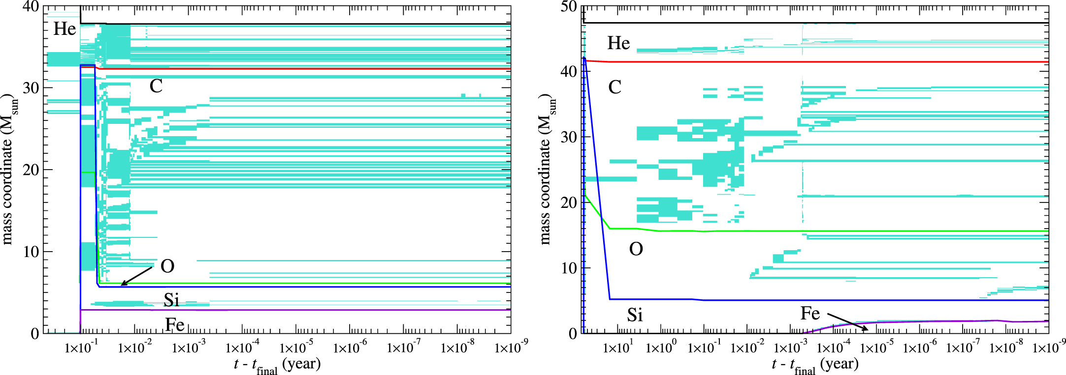
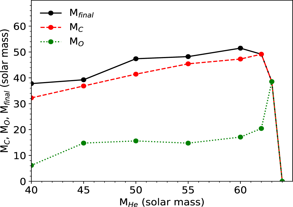
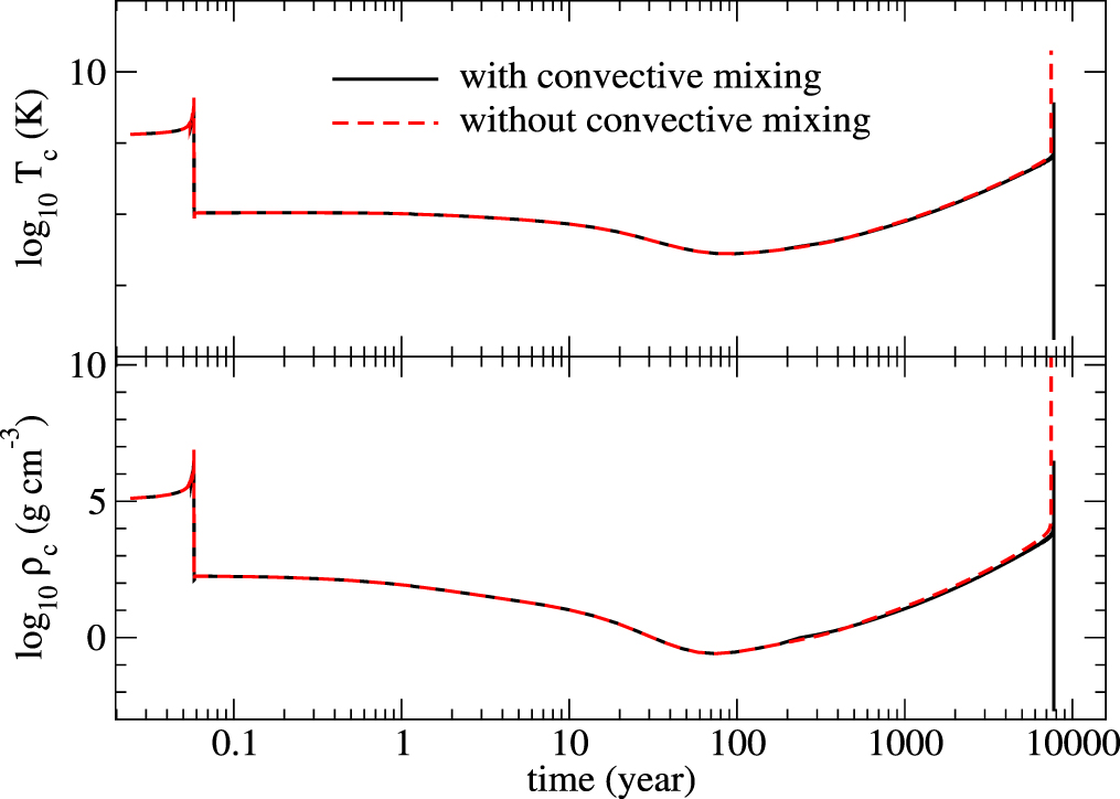
Figure 38. Left: the fluid velocity, speed of sound, and convective velocity of model He40A at Tc = 109.6 K. Right: the thermodynamic trajectory of model He40A with dynamical mixing (red dashed line) and without it (black solid line). The blue lines and the arrows have the same meaning as in Figure 14.
Download figure:
Standard image High-resolution image
As mentioned, switching on convection can be problematic in the hydrodynamics. To bypass this difficulty, instead of doing mixing in the hydrodynamics, we post-process the abundance profile at every step to mimic the mixing process. Similar to the standard MLT procedure, we first locate the mass shells that can undergo convection. Then we calculate the convection velocity and the corresponding mixing timescale tmix. After that, we compare with the time step Δt. If tmix < Δt, complete mixing is assumed; otherwise partial mixing among the cells in the convective zone is assumed. We notice that a consistent way to do the mixing process requires mixing entropy too. However, this affects the pressure, which in turn affects the dynamics. In fact, it is the mixing of fuel at the actively burning site that is important for triggering pulsation. As a first approximation, we neglect this complication.
In the right panel of Figure 38 we plot the thermodynamic trajectories of model He40A using the default prescription (no dynamical mixing) and the described mixing process. We can see that the two curves are very similar qualitatively. However, minor changes can be seen as small-scale pulses in the star. The model with dynamical mixing has fewer small pulses. The moment when the large pulse takes place differs. In the model without dynamical mixing it occurs at a higher Tc ∼ 109.8 K, while in that with dynamical mixing it occurs at a lower Tc ∼ 109.75 K. One possibility for this difference is that for a small pulse, the mixing tends to lower the 16O abundance available to the active burning site, which is more local. On the other hand, the mixing allows more zones to be rich in 16O when the star needs to carry out a collective burning of 16O. Therefore, this can occur earlier. Despite the difference it shows that the mixing process is efficient for lower-mass PPISNe but the replenishment of fuel does not particularly enhance the pulsation process.
Footnotes
- 5
We uploaded the related configuration files used in our simulations at doi:10.5281/zenodo.3457295.