


Abstract
Analysis of high-resolution Magnetospheric Multiscale Mission plasma and magnetic field data directly reveals the exchanges of energy between electromagnetic and flow energy and between microscopic flows and random kinetic energy in the inhomogeneous turbulent magnetosheath. The computed rates of exchange are based on exact results from the collisionless Vlasov model of plasma dynamics, without appeal to viscous or other closures. The description includes analyses of several structures observed in intervals of burst mode data in the magnetosheath, revealing pathways of energy exchange at sub-ion scales. Time-series of the work done by the electromagnetic field, and the pressure–stress interaction, enable description of the pathways to dissipation in this low-collisionality plasma. This method does not require any specific mechanism for its application, such as reconnection or a selected mode, although with increased experience it will be useful for distinguishing between proposed possibilities.
Export citation and abstract BibTeX RIS
1. Introduction
Plasma turbulence produces energy transfers across scales that drive, on balance, a transfer from large scales toward smaller scales. At kinetic scales, collective fluid motions degenerate eventually into heat. This sequence may be meaningfully described as "dissipation," even if some features are formally reversible, and even if many potentially identifiable mechanisms contribute to the overall process. It turns out, however, that the pressure–stress interaction is central for producing internal energy in all cases, whether collisional or collisionless. When collisions are dominant, the pressure–stress interaction takes a simple form due to a viscous closure. For weakly collisional plasma, that simple closure is not available, but the form of the pressure–stress interaction remains the same. This implies that the conversion of microscopic flows into internal energy, arguably the crucial link to dissipation, may be evaluated directly, provided that accurate pressure and stress measurements are available. At first, this statement may be uncomfortable for theorists, even though it follows from elementary manipulations of the Vlasov equation (Yang et al. 2017a), mainly because it skirts the complication that the pressure tensor is necessarily related to dynamics of higher-order moments. Some physical closure is required to close this problem in statistical theories. However, when the pressure tensor and stresses are known, their role in exchanges between internal energy and collective fluid motions becomes a potentially important factor, providing a description of dissipation activity not available from other typically measured quantities. This capability has not been fully exploited in the space plasma physics community.
The present paper makes use of the unique measurement capabilities of the Magnetospheric Multiscale Mission (MMS) to provide the first direct evaluation of the pressure–stress interaction and related quantities that govern energy conversion in space plasma. The hypothesis to be tested here is that the pressure–stress interaction, and the electromagnetic work on particles, provide mutually independent information related to energy conversion. We test this by direct evaluation of selected events in the turbulent magnetosheath. Our finding affirms that these diagnostics are indeed independent. Therefore, we conclude that, with further development, such measurements have the potential to provide a powerful tool for probing kinetic plasma behavior. This approach may help unravel many questions that surround dissipation and heating in low-collisionality space and astrophysical plasmas.
2. Energy Conversion Channels
For a collisionless plasma consisting of species labeled by α, the total energy density at each point  at a fixed time t consists of the electromagnetic energy density,
  , plus the sum over species of the individual particle kinetic energy densities
  . Here,
  and
and  are magnetic and electric fields, respectively, mα is the mass of particles of species α, and fα is the velocity distribution function of particles of type α, varying in position and time. The collective motion is quantified by the fluid velocity
  defined by
  , where
  is the number density of species α. Hereafter, we refer to these energy densities, for brevity, simply as energies.
Separating the kinetic energy into average and random parts facilitates our understanding of the energy conversion processes. The fluid flow kinetic energy of species α is  and the corresponding thermal (random) energy is
  , making it clear that
  .
.
The time evolution of the energies follows directly from standard elementary manipulations of the Vlasov equation and Maxwell's equations. The fluid flow energy evolves in time according to

Similarly, the time evolution equation for the internal kinetic energy of species α is

where  is the heat flux vector.
Finally, using the Maxwell curl equations, the equation governing  can be written as

where  is the total electric current density, and
  is the electric current density of species α.7
Several features of Equations (1)–(3) must be emphasized. First, all the terms grouped with the time derivatives on the left sides are transport terms that do not change the total amount of energy of the respective types, but simply move energy from one location to another. These transport terms integrate to zero for suitable boundary conditions and may be extremely important for reconciling the energy balance at any point in space and time. However, here we are less concerned with transport effects, as the emphasis is on quantifying conversion between different types of energy.8 Therefore, we will only discuss the terms on the right sides of these equations that are responsible for conversion of energy from one form to another.
Examining these terms, it is evident that the  terms convert electromagnetic energy into flow energy for each species α, and vice versa. All changes of the internal ("thermal") energy of each species are accomplished solely by the pressure–stress interaction, which we abbreviate as
  .
.
It should be emphasized that quantities such as  and PSα are not single-signed, as energy may be transferred into or out of the electromagnetic fields, and likewise into or out of the collective fluid motion of each species α. While the distributions of these quantities are not sign-definite, the expectation is that when there is net dissipation and heating, the appropriate sign indicating net transfer into random motions will be favored. This has been seen in magnetosheath observations (Retinò et al. 2007) and in plasma simulations in decaying turbulence (Wan et al. 2012; Yang et al. 2017a). Therefore, with some care, these quantities may be used to trace the flow of energy through different channels leading to dissipation.
Further decomposition is convenient. A standard procedure for decomposing the pressure tensor  and the stress tensor
  is to separate out the trace. One then defines
  , where
  . Similarly, the stress tensor is conveniently decomposed as
  , where
  and
and  are the symmetric and antisymmetric stress tensors, respectively. Then we see immediately that the pressure–stress interaction neatly separates as
  , where we have defined
  and the antisymmetric stress
  does not appear (Del Sarto et al. 2016).
A diagrammatic representation of the pathways to dissipation is shown in Figure 1. Overall, the transfer from scale-to-scale is believed, with substantial and growing empirical support, to proceed in a way that is analogous to the Kolmogorov cascade. Such cascades are driven by advective nonlinearities such as  for species α. These cascades are also expected to operate on both the incompressible and compressible degrees of freedom (Yang et al. 2016). A significant feature here is a separate velocity cascade for each species labeled by α. (Here, α will represent either protons α = p or electrons α = e.)
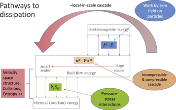
Figure 1. Diagram illustrating the pathways to dissipation outlined in the text. Velocity cascades transfer energy across spatial scales, a process expected to be dominated by Kolmogorov-like local-in-scale interactions. Electromagnetic work exchanges energy with the flow velocities of each species. The pressure–stress interactions convert kinetic energy between flows and internal energy. For a preliminary study of the scale dependence of these effects, see Yang et al. (2017b). Heat transport (not shown) moves internal energy in space but does not convert its form. For velocity implications, see Servidio et al. (2017).
Download figure:
Standard image High-resolution imageThe cascades, especially the incompressible parts, are widely viewed as approximately local in scale. In the pathways to dissipation there are other channels in addition to the velocity cascades. In the present paper, we are mainly concerned with the transfer between these channels. These channels—the work done on particles by the electromagnetic field, and the conversion between flow energy and internal energy—couple to the first moment, i.e., the flow velocities, and to the internal energy, that is, the second moments, of the velocity distributions. Other effects, not discussed here, contribute to anisotropies (Del Sarto et al. 2016) and higher-order moments of the particle velocity distribution functions. Eventually, this gives rise to a velocity space cascade (Schekochihin et al. 2016; Servidio et al. 2017), which then terminates through collisions and entropy production; these effects, however, require a model more complete than Vlasov–Maxwell (e.g., a Boltzmann model).
What we study below are quantities that participate in the termination of the inertial range cascade, while opening channels for production of velocity space excitations that lead eventually to collisional effects. In this sense the  and PS transfer channels provide the gateways between fluid scale effects and kinetic dissipation.
In the following sections, we demonstrate the use of  , pαθα, and PiDα as observational diagnostics in a turbulent magnetosheath. For discussions of the dynamics that control the evolution of the pressure tensor, see, e.g., Del Sarto et al. (2016), Del Sarto & Pegoraro (2018), and references therein.
3. MMS Data and Basic Calculations
For this demonstration we employ a single long-burst interval of MMS data, from 08:02:03 to 08:08:02 UTC on 2017 January 27, as the four spacecraft passed through Earth's turbulent magnetosheath.
From the MMS instruments on each spacecraft we can determine the pressure tensors and the total current density, as well as the electron and proton contributions to the current using data from the FPI instrument, the magnetic field from the FGM instrument, and the electric field from the EDP instrument. In addition, making use of the MMS multi-spacecraft configuration, we can determine the stress tensors  , or equivalently the trace-less tensor
  and the divergence
  for the relevant species. The stress determinations make use of techniques analogous to the "curlometer" technique (Dunlop et al. 2002). From the above quantities we can compute the pressure–stress interactions PSα, pαθα and PiDα, as well as
  , the contribution by species α to the electromagnetic work on the particles. For the present study we will consider only velocity distribution data for the electrons. Therefore, in all computations α → e, we will hereafter drop the subscript on the pressure–stress terms where no confusion is expected.
Figure 2 shows representative diagnostics for the entire 6-minute interval of magnetosheath turbulence under consideration. Shown (from top to bottom) are the vector magnetic field components (Bx, By, Bz) in GSE coordinates, the electron number density Ne, the electron temperatures Te (parallel, perpendicular, and total), the vector electron velocity components  , and the magnitude of the electron current, i.e., the electron contribution to the electric current density
  , magnitude of the total pressure–stress contraction PS, magnitude of pθ, and magnitude of PiD for electrons. The smallest-scale features resolved by the burst mode magnetic field data (@ 128 samples/s) and the burst mode electron data (@ 33.3 samples/s) are at sub-proton scales. The inter-spacecraft separation in this interval is the range of 5.5 km, which corresponds to a few times the electron inertial scale, and the mean plasma velocity is approximately 200 km s−1.
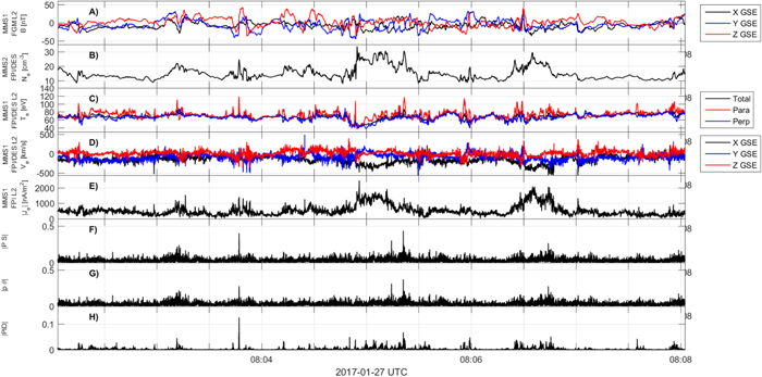
Figure 2. Overview of the 6-minute burst-resolution MMS observations in the turbulence of the Earth's magnetosheath on 2017 January 27. (A) Magnetic field in GSE coordinates. (B) Electron density. (C) Electron temperature (parallel, perpendicular, and total). (D) Electron velocity. (E) Magnitude of the electron current. (F) Magnitude of the total pressure–stress contraction PSe. (G) Magnitude of  . (H) Magnitude of PiDe.
Download figure:
Standard image High-resolution imageHere, the main purpose is to demonstrate how high-resolution MMS data may be employed to describe exchanges of energy between the different channels described in the previous section, for the weakly collisional turbulent magnetosheath. Based on the fundamental properties of the Vlasov–Maxwell system summarized in the previous section, and exploiting MMS measurement capabilities, one may distinguish between conversion of electromagnetic energy into flows, and conversion of microscopic flows into internal energy. This provides a novel view of the net effect of the many processes that may contribute to dissipation in space and astrophysical plasmas.
4. Energy Transfer at Intermittent Structures: Events
In the selected 6-minute interval, all measured quantities are highly fluctuating and exhibit bursty, intermittent behavior, as shown in Figure 2. Such turbulence is characterized by an abundance of small-scale structures that are sites of energy dissipation and particle energization (Sundkvist et al. 2007; Chasapis et al. 2015; Yordanova et al. 2016; Chasapis et al. 2017). The quantities defined in the previous section, calculated at the high resolutions provided by the MMS instruments, allow us to investigate the energy conversion within such structures.
Three such ion-scale intermittent structures are presented in Figures 3–5. All three are characterized by a sharp variation of the magnetic field, a strong current, and a coinciding significant increase in electron temperature, especially in the direction parallel to the magnetic field.

Figure 3. Ion-scale intermittent structure in the Earth's magnetosheath, highlighted in green and shown in the local reference frame of the structure (l, m, n), determined by minimum variance analysis and spacecraft timing. With respect to the GSE frame, the maximum variance component is l = (+0.0950, +0.6036, +0.7916), the out-of-plane direction is m = (+0.2453, +0.7565, −0.6063), and the normal direction is n = (−0.9648, +0.2518, −0.0762). The ratio of the eigenvalues corresponding to the intermediate and minimum variance components is 5.5. (A) Magnetic field. (B) Electron density. (C) Electron temperature, and its components parallel and perpendicular to local magnetic field. (D) Electron velocity along the l axis. (E) Electron current. (F)  , where
  is the electron current and
  is the electric field. (G) −PS; (H) −pθ; (I) −PiD, as defined in Section 2. In (F)–(I), the red and blue line segments denote positive and negative values.
Download figure:
Standard image High-resolution imageExamining the structure shown in Figure 3, we observe strong electron flows in the −l direction at the edges of the structure that coincide with the two positive spikes of  , indicating a transfer of energy from the electromagnetic field into particle energy. At the center of the structure, however, where the bulk of the parallel electron heating is observed, the evolutions of −PiD, −pθ, and −PS suggest that the hot electron population is not actively being heated but is cooling and expanding. This suggests a nearby source of energization, which resulted in the observed parallel heating, while at the point of observation, thermal energy is channeled into the flow as plasma expands and cools.
In the structure shown in Figure 4, we observe a similar behavior, with strong parallel electron heating. If only the magnetic field, electron temperatures, electron current, and  were analyzed, it seems likely one would again conclude that a site of magnetic reconnection is nearby. In fact, both of these events may be analyzed as potential reconnection events, exhibiting several of the standard features that such an identification would entail. However, our purpose here is not to discuss that interpretation in any depth.
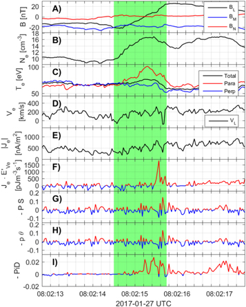
Figure 4. Ion-scale intermittent structure in the Earth's magnetosheath, highlighted in green and shown in the local reference frame of the structure (l, m, n), determined by a minimum variance analysis and spacecraft timing. With respect to the GSE frame, the maximum variance component was l = (−0.1734, −0.8457, +0.5047), the out-of-plane direction was m = (0.4036, 0.4064, 0.8197), and the normal direction was n = (−0.8984, +0.3458, +0.2708). The ratio of the eigenvalues corresponding to the intermediate and minimum variance components is 8. The quantities shown in each panel are the same as those in Figure 3.
Download figure:
Standard image High-resolution imageWhat we do want to point out is that the Figure 4 event involves subtle differences in comparison to the Figure 3 event. In particular, the behaviors of −PiD, −pθ, and −PS are different. These are again shown as the bottom three panels of the figures. In the case of Figure 4, while −pθ and −PS fluctuate, −PiD has a positive sign. That suggests an increase of the thermal energy of the electrons at the point where the MMS spacecraft is, pointing to a region of active electron heating.
We observe that the pressure–stress interactions provide new information that is unavailable in the other more standard diagnostics. The ability to discern whether internal energy is being increased by the dynamics, or decreased, on a point-by-point basis, can now enable more complete interpretations with MMS's ability to provide both the  and the pressure–stress diagnostics.
As a last example, shown in Figure 5, we present once again a similar sheared magnetic profile, with a strong electron current and an associated significant elevation of parallel electron temperature. Without the new diagnostics, such an elevation of temperature might be routinely associated with heating. In this case, however, −PiD, −pθ, and−PS are mostly negative throughout the traversal of the structure, indicating that local dynamics is cooling the plasma, even if the local temperature is, at this moment, higher than the surroundings. Recall that transport of heat (through conduction or advection) is not quantified here, although these may be contributors to elevated temperature. However. neither conduction nor advection of internal energy can cause local conversion into internal energy as these quantities transport heat energy but do not convert it into (or out of) other forms. Additionally, an increase of the electron velocity in the −l direction is observed along with an oscillating, but mostly negative (after about 08:02:58)  . Furthermore, flow energy in the observed fast (∼100 km s−1) streams is being converted into magnetic field energy, consistent with the above interpretation. This event may not be of a type that can be analyzed in terms of magnetic reconnection. Rather, it seems to be a flux tube interaction involving previously compressed plasma that is now expanding and amplifying the magnetic field. Evaluation of the pressure–stress interactions again can help to complete and clarify the nature of the dynamics in this interval.

Figure 5. Ion-scale intermittent structure in the Earth's magnetosheath, highlighted in green and shown in the local reference frame of the structure (l, m, n), determined by a minimum variance analysis and spacecraft timing. With respect to the GSE frame, the maximum variance component was l = (−0.0480, +0.9794,−0.1961), the out-of-plane direction was m = (−0.4397, +0.1556, +0.8846), and the normal direction was n = (+0.8969, +0.1287, +0.4232). The ratio of the eigenvalues corresponding to the intermediate and minimum variance components is 21. The quantities shown in each panel are the same as those in Figure 3.
Download figure:
Standard image High-resolution image5. Correlations: Joint Distribution Functions
Using MMS measurement capabilities in the magnetosheath, we now provide a statistical characterization of symmetric stress and its relationship to vorticity and electron current density, as well as the distribution of the pressure–stress interaction in the magnetosheath.
By way of background, it has been noted by several authors (Greco et al. 2012; Servidio et al. 2012; Karimabadi et al. 2013; Chasapis et al. 2017) that kinetic effects, including anisotropies, preferentially occur in the vicinity of concentrated electric current density. However, this does not imply that these kinetic effects occur at the precise locations of current sheets or other current concentrations. This is consistent with test particle orbit calculations (Dmitruk et al. 2004; Dalena et al. 2014) that find that particle energization often occurs near current sheets in regions of strong flow inhomogeneity and associated inhomogeneity of the induced electric field). Even more generally, enhancements of kinetic activity, including dissipation and energization, tend to be stronger at positions at which there are strong gradients in at least one of the plasma variables, such as magnetic field, velocity field, or density. Indicators such as partial variance of increments (Greco et al. 2009) become large at such locations, as seen in both simulations and solar wind data sets (Servidio et al. 2014).
The proximity of proton heating and strong gradients is at least partially due to the connection between proton pressure anisotropy and vorticity (Del Sarto et al. 2016) and the association of regions of elevated temperature (Franci et al. 2016) with vorticity. These lines of reasoning converge when one notices that quadrupolar regions of vorticity are formed dynamically near reconnecting current sheets (Matthaeus 1982; Parashar & Matthaeus 2016).
This leaves an apparent puzzle as to how vorticity can enter into localization of heating, given that the vorticity is related to the antisymmetric stress  , while only symmetric stress
  enters in the pressure–stress interactions PijSij. Therefore, in spite of the above statistical associations, vorticity cannot directly cause an increase in internal energy. However, statistics from the kinetic plasma simulations (Parashar & Matthaeus 2016; Yang et al. 2017b) reveal the following associations, which serve to clarify these issues: (a) there is a lack of positive correlation (and a possible inverse correlation) between symmetric stress and electron current density, and (b) there is a striking positive correlation between symmetric stress and vorticity. The former of these supports the idea that drivers of pressure–stress interaction are only slightly separated from current sheet maxima. The latter association is readily understood if the sheared velocity structures are quasi-two-dimensional and very sheet-like.
We now show that very similar correlations and statistical distributions are found in the magnetosheath.
First, in Figure 6 we show a joint distribution (scatter plot) of "the square of electron current density" (≈ second invariant of the antisymmetric magnetic stress tensor) versus the second invariant  of the symmetric stress. These are measures of the strength of local electron current density, and of symmetric stress, respectively. It is apparent that this joint distribution shows no systematic positive correlation, and that the larger symmetric stress values tend to occur at positions where the electron current is smaller, and vice versa. This is consistent with the findings reported by Yang et al. (2017b) based on kinetic PIC simulation.

Figure 6. Scatter plot of  vs. Qd, for electrons, in the magnetosheath interval shown in Figure 2. The apparent lack of positive correlation (and possible inverse correlation) is similar to that found in the kinetic PIC simulation of Yang et al. (2017b).
Download figure:
Standard image High-resolution imageFigure 7 shows a scatter plot (joint distribution) of Qd and the collocated values of the square of vorticity  where
where  . Here, it is immediately clear that these quantities are highly correlated—larger values of vorticity tend to occur where there are also larger values of symmetric stress. This is also consistent with the correlations of the same quantities found in PIC simulation Yang et al. (2017b).
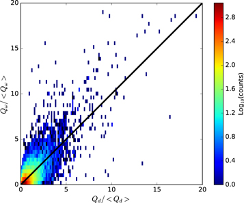
Figure 7. Scatter plot of Qω vs. Qd, for electrons, in the magnetosheath interval shown in Figure 2 The apparent positive correlation is consistent with that seen in the PIC simulation of Yang et al. (2017b).
Download figure:
Standard image High-resolution imageAs a final statistical perspective on the pressure–stress interactions, we compute the associated probability distribution functions (PDFs) from the MMS full burst interval. Figure 8 illustrates the PDFs of the pressure–stress terms, −PS, −pθ, and −PiD for the same burst interval employed above. It is readily apparent that the full pressure–stress interaction PS as well as the compressible ingredient pθ, and the shear associated PiD, are broadly distributed and are not single-signed. Therefore, the pressure–stress interactions in the magnetosheath can convert energy into internal energy from electron flows, and conversely, can convert internal energy into flows, the two processes occurring with almost equal frequency in this data set. There is, however, a slight positive excess, indicating a net heating, or increase of internal energy.

Figure 8. Probability distribution functions of −PS, −pθ, and −PiD for electrons, in the magnetosheath interval shown in Figure 2.
Download figure:
Standard image High-resolution image6. Discussion
The purpose of the present paper has been twofold: (1) to demonstrate how the energy exchange channels discussed by Yang et al. (2017a) may be used to describe plasma dynamics; and (2) to show how the high-resolution multi-spacecraft instrumentation on the MMS mission provides essentially all the information needed to implement this approach to the description plasma dynamics at kinetic scales.
The present demonstration, in Earth's magnetosheath, shows that a more complete perspective is achieved when one can distinguish between energy gain or loss by microscopic plasma flows for each species, and gains or loss of random (or thermal) kinetic energy in the same species.
Here, we illustrated this approach in observational data, complementing previous implementations of this approach in kinetic plasma simulations (Yang et al. 2017a, 2017b). The examples shown from MMS data employed only electron data.
We conclude that an analysis based on scale-to-scale cascades (not explored here; however, see Yang et al. (2016) for the MHD case), along with the full array of electromagnetic work diagnostics  , and the full array of pressure–stress interactions (pressure dilatation as well as PiD for each species), could potentially provide essentially complete maps of energy transfer in scale and between channels. This approach may prove to be quite valuable for tracking down the specific processes that contribute to dissipating fluctuations in collisionless plasmas. The only remaining factors, those involved in spatial transport, present different and equally important challenges.
This research is partially supported by the MMS mission through NASA grant NNX14AC39G, and NASA Grand Challenge Theory program grant NNX14AI63G, at the University of Delaware, and NSF-SHINE AGS-1460130. A. Chasapis is supported by the MMS grant. Y. Y. acknowledges support by the China Scholarship Council. W.H.M. is a member of the MMS Theory and Modeling team. We thank an anonymous referee for persistent criticisms that led to improvements of the presentation. We acknowledge the assistance of the MMS instrument teams, especially FPI and FIELDS, in preparing the data, as well as the work done by the SDC. The data used in this analysis are Level 2 FIELDS and FPI data products, in cooperation with the instrument teams and in accordance their guidelines. All MMS data are available at https://lasp.colorado.edu/mms/sdc/.
Footnotes
- 7
Some readers may prefer to use terminology such as "thermal energy" or "random kinetic energy" to refer to the quantity
 .
. - 8
We do not suggest that transport effects such as heat flux and convective heat transport are small, as in many circumstances these are significant or even dominant contributions to the balance of Equation (2); however, these terms do not exchange energy between different forms, and it is the exchange between different pathways or channels that is our main interest here.
