


ABSTRACT
We present results from a very deep (650 ks) Chandra X-ray observation of the galaxy group NGC 5813, the deepest Chandra observation of a galaxy group to date. This system uniquely shows three pairs of collinear cavities, with each pair associated with an unambiguous active galactic nucleus (AGN) outburst shock front. The implied mean kinetic power is roughly the same for each outburst, demonstrating that the average AGN kinetic luminosity can remain stable over long timescales (∼50 Myr). The two older outbursts have larger, roughly equal total energies as compared with the youngest outburst, implying that the youngest outburst is ongoing. We find that the gas radiative cooling rate and mean shock heating rate are well balanced at each shock front, suggesting that shock heating alone is sufficient to offset cooling and establish AGN/intracluster medium (ICM) feedback within at least the central 30 kpc. This heating takes place roughly isotropically and most strongly at small radii, as is required for feedback to operate. We suggest that shock heating may play a significant role in AGN feedback at smaller radii in other systems, where weak shocks are more difficult to detect. We find non-zero shock front widths that are too large to be explained by particle diffusion. Instead, all measured widths are consistent with shock broadening due to propagation through a turbulent ICM with a mean turbulent speed of ∼70 km s−1. Finally, we place lower limits on the temperature of any volume-filling thermal gas within the cavities that would balance the internal cavity pressure with the external ICM.
Export citation and abstract BibTeX RIS
1. INTRODUCTION
Early Chandra and XMM-Newton X-ray observations revealed that the amount of gas cooling to very low temperatures at the centers of cool core clusters is much less than what is expected from simple radiative cooling models (David et al. 2001; Peterson et al. 2001; Fabian et al. 2006). The implication is that the diffuse X-ray-emitting gas must be heated, either by pre-heating during cluster formation or by ongoing energy injection. The most likely heating mechanism is feedback due to energy injection by the central active galactic nucleus (AGN) of the cD galaxy (see McNamara & Nulsen 2007; Fabian 2012). During this process, matter is accreted onto the central supermassive black hole (SMBH), which drives powerful jets. These jets evacuate cavities in the intracluster medium (ICM), which can drive shocks as they are inflated and subsequently rise buoyantly (Churazov et al. 2001). The energy contained in cavities and shocks is then available to heat the ICM, which lowers the cooling rate of the gas and subsequently the SMBH accretion rate. The ensuing decrease in AGN heating allows the gas to once again cool and accrete onto the SMBH, establishing a feedback loop that regulates the temperature of the ICM. Several studies have shown that, generally, the total enthalpy in cavities in cool core systems is sufficient to offset radiative cooling in individual galaxies, galaxy groups, and clusters (Bîrzan et al. 2004; Rafferty et al. 2006; Nulsen et al. 2007; Hlavacek-Larrondo et al. 2012). However, the details of how and where this energy gets transferred to the ICM are unclear. Weak AGN outburst shocks are also expected to heat the ICM, although they are difficult to detect and clear examples are very rare.
Galaxy groups provide an excellent opportunity to study AGN feedback. Their lower temperatures are more easily measured with modern high angular resolution X-ray satellites, and their central AGN can more easily disturb the diffuse gas due to their shallower gravitational potentials as compared with clusters. Here we report on results from a very deep Chandra observation of the central galaxy in the galaxy group NGC 5813 (N5813). This group is a relatively isolated sub-group in the NGC 5846 group (Mahdavi et al. 2005; Machacek et al. 2011). In Randall et al. (2011, hereafter R11) we presented results based on an initial 150 ks Chandra observation of N5813. The ICM in this group has a remarkably regular morphology, with three pairs of roughly collinear cavities and associated surface brightness edges, and shows no clear signs of a recent merger event. (Note that we refer to the diffuse gas in this group as the ICM rather than the intragroup medium [IGM] throughout to stress the connection with feedback in clusters and to avoid confusion with the intergalactic medium.) With clear, cleanly separated signatures from three distinct outbursts of the central AGN and no other significant dynamical processes at work, N5813 is uniquely well suited to the study of AGN feedback. In this work, we focus on the implications for AGN feedback and the outburst history of the central SMBH.
We assume an angular diameter distance to N5813 of 32.2 Mpc (Tonry et al. 2001), which gives a scale of 0.15 kpc arcsec−1. All uncertainty ranges are 68% confidence intervals (i.e., 1σ), unless otherwise stated.
2. CHANDRA DATA ANALYSIS
2.1. Observations and Data Reduction
The Chandra observations that were used in the analysis we present here are summarized in Table 1. The aimpoint was on the back-side-illuminated ACIS-S3 CCD for each observation. All data were reprocessed from the level 1 event files using CIAO and CALDB 4.4.3. CTI and time-dependent gain corrections were applied. lc_clean was used to remove background flares.9 The mean event rate was calculated from a source-free region using time bins within 3σ of the overall mean, and bins outside a factor of 1.2 of this mean were discarded. There were no periods of strong background flares. The cleaned exposure times are given in Table 1, for a total time of 635 ks.
Table 1. Chandra X-Ray Observations
| Obs ID | Date Obs | CCDs Used | Cleaned Exposure |
|---|---|---|---|
| (ks) | |||
| 5907 | 2005 Apr 2 | S1, S2, S3, I3 | 48.1 |
| 9517 | 2008 Jun 5 | S1, S2, S3, I3 | 98.3 |
| 12951 | 2011 Mar 28 | S1, S2, S3, I2, I3 | 73.7 |
| 12952 | 2011 Apr 5 | S1, S2, S3, I2, I3 | 142.3 |
| 12953 | 2011 Apr 7 | S1, S2, S3, I2, I3 | 31.7 |
| 13246 | 2011 Mar 30 | S1, S2, S3, I2, I3 | 45.0 |
| 13247 | 2011 Mar 31 | S1, S2, S3, I2, I3 | 35.7 |
| 13253 | 2011 Apr 8 | S1, S2, S3, I2, I3 | 116.7 |
| 13255 | 2011 Apr 10 | S1, S2, S3, I2, I3 | 43.0 |
Download table as: ASCIITypeset image
Diffuse emission from N5813 fills the image field of view (FOV) for each observation. We therefore used the CALDB
10
blank sky background files appropriate for each observation, normalized to match the 10–12 keV count rate in our observations to account for variations in the particle background. To generate exposure maps, we used a MEKAL model with  keV, Galactic absorption, and abundance of 30% solar at a redshift
  .
.
3. IMAGE ANALYSIS
The exposure-corrected, background-subtracted, 0.3–3 keV Chandra image of the central region is shown in Figure 1. To enhance the visibility of the diffuse emission, bright point sources were removed, and the regions containing point sources were "filled in" using a Poisson distribution whose mean was equal to that of a local annular background region. To better show faint structure, particularly in the outer regions, we fitted the X-ray image with a 2D beta model using the software package sherpa (Freeman et al. 2001) and divided the image by the model to produce a residual image. The smoothed, point-source-free image and the residual image are shown in Figure 2.

Figure 1. Exposure-corrected, background-subtracted, 0.3–3 keV Chandra image of the central region of N5813, unsmoothed and with point sources included (1 pixel = 0  5).
5).
Download figure:
Standard image High-resolution image
Figure 2. Left: exposure-corrected, background-subtracted, 0.3–3 keV Chandra image, with point sources removed and smoothed with a  Gaussian. The image shows bright rims surrounding an inner pair of cavities, a prominent elliptical edge surrounding a pair of cavities at intermediate radii (with the more obvious cavity to the SW and the NE cavity apparently broken into two connected cavities), and a subtle outer edge associated with a faint pair of outer cavities (with the more obvious cavity to the NE). Right: X-ray image divided by a 2D fitted beta model and smoothed with a
  '' Gaussian, shown on the same scale. The outer cavities and edges are more clearly seen in this residual image, while the inner cavities are not visible due to the larger smoothing scale and saturation of the color scale. The image also reveals a faint "channel" of decreased surface brightness extending to the north, apparently connected to the NE outer cavity.
Download figure:
Standard image High-resolution imageThese images clearly show three pairs of roughly collinear cavities, along an axis from the SW to the NE. The inner cavity pair is surrounded by bright rims (at about 1 kpc), and each of the intermediate and outer cavity pairs is associated with an elliptical surface brightness edge (at ∼10 and ∼30 kpc, respectively). In R11, we showed that the 1 and 10 kpc edges are shock fronts that were driven during the expansion phase of their associated cavities. The new, deeper observations clearly show a third (outer) cavity pair and edge, only hinted at in earlier observations, and allow us to unambiguously identify the outer edge as an associated shock front (Section 4.2.2). These outer features are most clearly seen in the residual image (Figure 2). Thus, these deep X-ray observations show clear signatures from three distinct outbursts of the central AGN. We note that, here and throughout, by "outburst" we refer to the creation of a cavity pair and its associated shocks, rather than a rapid increase in AGN jet power, since these features are in principle consistent with either a constant or variable jet power (see Section 6.2).
To look for structure in the faint emission at large radii, beyond the FOV of Chandra, we examined the available archival XMM-Newton observations of N5813. N5813 was observed with XMM-Newton on three occasions: 2005 July 23 (ObsID 0302460101), 2009 February 11 (ObsID 0554680201), and 2009 February 17 (ObsID 0554680301). The event files were calibrated using the XMM-Newton Science Analysis System version 13.5.0 and the most recent calibration files as of 2014 July. The calibrated, cleaned event files were produced after filtering for particle background flares. This resulted in cleaned exposure times of 120, 127, and 83 ks for the MOS1, MOS2, and PN detectors, respectively. Details of the data reduction are described in Bulbul et al. (2012a).
The background-subtracted, exposure-corrected, merged XMM-Newton image is shown in Figure 3 beside the Chandra image. The 10 kpc shock edges are visible, as are the intermediate cavities and the NE outer cavity. The inner ∼1 kpc cavities and rims are not resolved. A smoothed version of this image, with the intensity scale chosen to better show faint emission at large radii, is shown in Figure 4. The extended emission is roughly azimuthally symmetric and shows no clear evidence of a fourth pair of cavities or shock edge beyond the 30 kpc edge detected with Chandra. Since, for the purposes of this study, we are most interested in the detailed structure in the ICM, which is best resolved with Chandra, we will not consider the XMM-Newton data further here.

Figure 3. Left: background- and exposure-corrected 0.4–7.2 keV XMM-Newton image of N5813. Right: smoothed Chandra image shown on the same scale, with the intensity scale chosen to better show the faint, outer emission.
Download figure:
Standard image High-resolution image
Figure 4. XMM-Newton image shown in Figure 3, smoothed and with the intensity scale chosen to show the faint emission at large radii beyond the Chandra FOV. There are no additional cavities or shock edges visible beyond the inner features identified in the Chandra images.
Download figure:
Standard image High-resolution image4. SPATIALLY RESOLVED SPECTROSCOPY
Unless otherwise specified, all spectra were fitted in the 0.6–3.0 keV band using xspec, with an absorbed apec model with the absorption fixed at the Galactic value of  cm−2 (Kalberla et al. 2005) and the abundance allowed to vary. Spectra were grouped with a minimum of 40 counts per energy bin. Anders & Grevesse (1989) abundance ratios and AtomDB 2.0.2 were used throughout. We note that using this version of AtomDB gives systematically larger temperatures (by roughly 0.05–0.1 keV, significantly larger than our typical statistical error) as compared with AtomDB 1.3.1, which was used in R11. This difference arises from significant changes in the ionization balance, particularly at the low (∼0.7 keV) temperatures we consider here (see Figure 3 in Foster et al. 2012). Thus, we expect a systematic offset between the spectroscopic quantities that we derive here as compared with R11.
4.1. Spectroscopic Maps
To study the thermal structure of the ICM, we generated a smoothed temperature map using the method described in Randall et al. (2008) and also used in R11. For each pixel in the temperature map, spectra were extracted from a surrounding circular region that contained 1500 source counts. The temperature map pixel value was then set equal to the best-fitting temperature from fitting to these spectra. Since the extraction regions are generally larger than the pixels, nearby pixels are correlated with one another, such that the temperature map is effectively smoothed on the scale of the local extraction region size. Some advantages of this method are that there is no a priori assumption about the thermal structure of the gas, and experience has shown that such maps can resolve real structure on scales that are smaller than the size of the extraction regions.
For comparison, we also constructed temperature maps using the contour-binning method developed by Sanders (2006). Here, extraction regions are defined based on surface brightness contours. Regions were defined to achieve a signal-to-noise ratio of 38 (corresponding to ∼1400 counts in bright regions) in each region. This method assumes that the temperature distribution follows the surface brightness distribution (which is frequently, but not always, the case). Some advantages of this method are that each extraction region is independent of the others (as long as the region widths are large compared with the local point-spread function [PSF]), and it is relatively cheap computationally (as compared with the smoothed temperature map method). A comparison of the smoothed and contour binned temperature maps gives an indication of the extraction region size as a function of position in the smoothed map.
Smoothed temperature maps over a wider area and a higher-resolution map of the core are shown beside the contour-binned maps in Figures 5 and 6, respectively. Both the smoothed and contour-binned temperature maps reveal relatively hot emission associated with the bright rims surrounding the inner cavities and just inside the prominent 10 kpc surface brightness edges. These features were identified as shocks in R11. The maps suggest additional temperature rises associated with the outer 30 kpc surface brightness edges, particularly to the NW. The temperature profiles across these edges are presented in Section 4.2.2. The temperature maps also show a plume of cooler gas, roughly extending along the line defined by the cavities, from SW to NE. In R11, we showed that this plume is consistent with arising from cool gas that has been lifted by the buoyantly rising X-ray cavities.

Figure 5. Smoothed (left) and contour-binned (right) temperature maps. The locations of the 10 and 30 kpc shock fronts are indicated with dashed black lines, and the cavity locations with black ellipses. Both maps clearly show temperature increases associated with the 1 and 10 kpc shocks and hint at increases associated with the 30 kpc shock (particularly to the NW). Also visible is an SW to NE plume of cool gas that has been uplifted by the buoyantly rising cavities.
Download figure:
Standard image High-resolution image
Figure 6. Left: high-resolution smoothed temperature map of the core region. Right: contour binning temperature map shown on the same scale. The 10 kpc shock fronts are indicated as in Figure 5.
Download figure:
Standard image High-resolution imageWe derived pseudo-pressure and pseudo-entropy maps from the smoothed temperature maps. The fitted apec normalization for each spectral map pixel is proportional to the volume integral of the square of the electron density along the line of sight. The square root of the normalization therefore gives an average "projected" density along the line of sight. We define the pseudo-pressure and pseudo-entropy as  and
and  , respectively, where kT is the fitted projected temperature and A is the normalization scaled by the area of the extraction region. The wide field and core maps are shown in Figures 7 and 8. The pseudo-pressure maps reveal prominent pressure jumps across the 10 kpc shock fronts and increased pressure in the bright central rims (i.e., the 1 kpc shock). There is no obvious equivalent structure in the pseudo-entropy maps. This is not unexpected for weak shocks. For the strongest shock we detect, with
  , the Rankine–Hugoniot shock jump conditions for a
  gas give a pressure jump at the shock front of a factor of 3.7, but a jump in the entropy index of only a factor of 1.12. Thus, entropy jumps are expected to be relatively difficult to detect, particularly in projection.

Figure 7. Pseudo-pressure (left) and pseudo-entropy (right) maps, in arbitrary units. The pressure map was calculated as  and the entropy map as
  , where A is the apec normalization scaled by the area of the extraction region. Shocks and cavities are indicated as in Figure 5. The pressure jumps are visible at the 1 and 10 kpc shock fronts. There are no visible entropy jumps at the shock fronts, consistent with the expectation that entropy jump amplitudes are small for weak shocks compared with those of the temperature and pressure jumps.
Download figure:
Standard image High-resolution image
Figure 8. Pseudo-pressure (left) and pseudo-entropy (right) maps corresponding to the smoothed temperature map of the core shown in Figure 6 (with the same regions overlaid), created as in Figure 7. Pressure increases are clearly seen at the 10 kpc shock fronts and in the bright, shock-heated rims surrounding the inner cavity pair. There is some structure visible in the core of the pseudo-entropy map (seen in blue as filament-like structures), likely resulting from central gas that has been pushed out and uplifted from the core by the expanding and rising X-ray cavities.
Download figure:
Standard image High-resolution imageThe core pseudo-entropy map (Figure 8) shows some filamentary structure in the center, on the scale of the bright shocked rims. However, unlike the features in the pseudo-pressure map, these features do not directly trace the bright rims. Furthermore, the entropy is lower in these filaments as compared with the surrounding regions, in contrast to the small increase in entropy that is expected at the shock fronts. These structures are likely formed as the central low-entropy gas is pushed and pulled away from the center as the inner cavities expand and rise buoyantly.
The central regions of the core temperature and pseudo-entropy maps are shown with the Hα contours from R11 overlaid in Figure 9. As shown in R11, the Hα emission follows the plume of cool X-ray-emitting gas up to the location of the intermediate cavities, indicating that these cavities have uplifted cold-phase gas from the core as they buoyantly rise. The Hα emission also clearly traces the SW inner cavity, suggesting that the central cold-phase gas is dynamically coupled to the cavity and is being pushed out as the cavity expands. The SE 1 kpc shock appears to be passing through the Hα filament (at least in projection) without destroying it. Finally, there is a correlation between the Hα emission and the detailed, small-scale, filamentary structure of the central low-entropy gas. This is consistent with the above suggestion that these entropy features likely arise from gas that has been displaced from the core by the cavities, rather than from entropy changes driven by the central shocks.

Figure 9. Core temperature (left) and pseudo-entropy (right) maps with Hα contours from R11 overlaid. Units are keV for temperature and arbitrary for entropy. The SE 10 kpc shock is indicated by the dashed line. The Hα emission follows the cool plume of gas up to the intermediate cavities and traces the SW inner cavity. There is a correlation with the detailed, filamentary structure of the central low-entropy gas in the pseudo-entropy map (e.g., with the low-entropy filament just NE of the core).
Download figure:
Standard image High-resolution imageSince each extraction region in the above maps contained only 1500 net counts, the abundance values determined by these fits were not tightly constrained, and the corresponding abundance maps show little to no structure. Abundance measurements in ∼0.7 keV gas are challenging due to the large number of closely spaced emission lines and the resulting degeneracy between line and continuum emission at Chandra's energy resolution. We found that, for N5813, achieving 1σ errors on the order of 5%–10% for the abundance required roughly 30,000 net counts. Fortunately, the new deeper observations provided well over one million photons appropriate for use in spectral fitting, allowing us to map the abundance distribution in the gas. A smoothed abundance map, with 30,000 net counts per extraction region, is shown in Figure 10.

Figure 10. Smoothed abundance map, with cavity and shock regions overlaid as in Figure 5. The apparent low abundance in the plume of uplifted cool gas (extending NE and SW of the core) is an artifact of fitting a single-temperature model to multi-temperature spectra (see text).
Download figure:
Standard image High-resolution imageThe abundance map shows an apparent plume of low-abundance gas that corresponds to the plume of uplifted cool gas seen in Figure 5 (roughly 40 kpc long, extending from SW to NE). It has long been recognized that fitting multi-temperature spectra with a single thermal model can give anomalously low abundance values (the so-called "Fe-bias" effect; Buote 1999). To test for this effect, we fit multi-temperature models to the apparent central minimum and apparent low-metallicity NE plume. We find that the plume is well described by a two-temperature model, with  keV,
keV,  keV, and an abundance (set equal for each temperature component) of
  % solar, consistent with the surrounding ICM. In contrast, we find that, while including multiple temperature components for the central region (in a
  kpc ellipse oriented NE to SW, along the plume) does raise the fitted abundance, it is still significantly lower than the abundance of the surrounding ICM, at
  % solar. Thus, we conclude that the apparent low abundance in the extended plume is a fitting artifact arising from the Fe-bias effect, and that the measured abundance in the plume is consistent with that of the surrounding ICM, while the apparent abundance minimum within the central few kpc cannot be easily explained by this effect. We note that central abundance dips that apparently cannot be explained solely by projection effects have been seen in other systems (e.g., Blanton et al. 2003; Panagoulia et al. 2013). In addition to the apparent low-abundance plume, there appear to be increases in the projected abundance at the location of the shock fronts, in contradiction with what is expected from the Fe-bias effect. A more detailed study of these features and the ICM abundance in general in N5813 will be presented in an upcoming paper.
4.2. Radial Profiles
4.2.1. Azimuthally Averaged Profiles
We produced projected radial profiles by fitting spectra extracted from concentric annuli, centered on the centroid of the diffuse emission at large radii. Each annulus was chosen to be at least 1'' wide and contain at least 1000 net counts in the 0.6–3.0 keV band. The inner annuli were limited by the size constraint (and therefore contained more than 1000 net counts), whereas the outer annuli were wider and contained roughly 1000 net counts. The resulting temperature profile is shown in the top panel of Figure 11. The positions of the shock fronts (determined in Section 5) are marked by vertical lines. Even in the projected temperature profile in circular annuli (which effectively smooths out the elliptical shock fronts), temperature enhancements associated with each shock are clearly visible. The central 15 radius region, which contains the central AGN, has been excluded from the fit to the central region. The central temperature rise is due to the presence of the inner shock rims surrounding the inner cavities.

Figure 11. Azimuthally averaged radial profiles for (top to bottom) temperature, electron density, pressure, and entropy, extracted from circular annuli. The top panel shows the projected (black circles) and deprojected (red triangles) temperature profiles. All other panels show deprojected values. The vertical lines mark the positions of the shock fronts to the SE (dotted) and NW (dashed) determined by fits to the surface brightness profiles in sectors (see Section 5). Increases in temperature associated with each pair of shock fronts (i.e., each full elliptical edge) are clearly seen even in the azimuthally averaged, projected temperature profile. The "kink" in the deprojected profiles is likely due to the breakdown of the assumption of spherical symmetry at the location of the bright, sharp shock edges at ∼10 kpc.
Download figure:
Standard image High-resolution imageAs in R11, we determined the 3D structure of the ICM by performing an "onion peeling" deprojection analysis (Fabian et al. 1981) using concentric annuli, each of which contained at least 8000 net counts (in projection) in the 0.6–3.0 keV band. We fit each annulus with an absorbed apec model, with the abundance fixed at 50% solar (consistent with results from spectral fits to the total diffuse emission and with typical values in the projected abundance map shown in Figure 10). We assume spherical shells of uniform density. Given the rich morphology of N5813, with elliptical shock edges, cavities, and other features, it is clear that the assumption of spherical symmetry does not strictly apply. Thus, the deprojected profiles include some level of systematic uncertainty associated with the assumed geometry. The deprojected temperature, density, pressure, and entropy profiles are shown in Figure 11. We see that the deprojected temperature is generally consistent with the projected temperature. We interpret this an indicating that the scale of the azimuthally averaged temperature gradient is generally small compared with the sizes of our extracted annuli, so that projection effects in any given annulus (which are dominated by emission from adjacent annuli) are relatively small. The small discontinuous jumps, or "kinks," in the density, pressure, and entropy profiles around 11 kpc are associated with the sharp surface brightness edges to the NW and SE from the intermediate shock.
4.2.2. Shock Front Profiles
To confirm the temperature rises across the surface brightness edges seen in Figures 5 and 6, we derived temperature profiles in annular bin sectors across each of the edges. The profiles were centered on the center of curvature for each feature (such that there was a bin boundary that traced the surface brightness edge), and then the distances were corrected to measure the distance from the center adopted for the azimuthal profiles presented in Section 4.2.1.
The temperature profiles across the 10 and 30 kpc shock fronts are shown in Figures 12 and 13, respectively, with the fitted shock front positions overlaid (see Section 5). Clear temperature rises are seen at each front, confirming that these features are shocks. In the case of the 10 kpc shocks, the deeper observations allow us to measure the temperature profiles with greater angular resolution (on the scale of a few hundred pc) as compared with R11. In addition to the overall shift in normalization due to the updated AtomDB (see Section 4), the peak change in temperature across the fronts is larger as compared with the more coarsely binned profiles in R11. In contrast, the shock Mach numbers that we derive here (Section 5) are consistent with those derived in R11, since the surface brightness profile requires fewer counts per radial bin, allowing for smaller bins. This is consistent with our suggestion in R11 that the temperature jumps we found there were smaller than what was expected based on the Mach numbers derived from the surface brightness jumps due to projection effects.

Figure 12. Projected temperature profiles across the NW (left) and SE (right) 10 kpc shock fronts. The dashed lines indicated the fitted shock front positions.
Download figure:
Standard image High-resolution image
Figure 13. Projected temperature profiles across the NW (left) and SE (right) 30 kpc shock fronts. The dashed lines indicated the fitted shock front positions.
Download figure:
Standard image High-resolution imageIn some cases, there appears to be shock-heated gas just outside the positions of the shock front (e.g., the two bins to the right of the edge in Figure 12, left). There are at least two factors that can contribute to this effect. First, there is a small uncertainty in the fitted locations of the shock fronts. Second, we show in Section 5 that the shock fronts have finite widths (on the order of 0.5 kpc for the 10 kpc shock). When fitted with a discontinuous model, the preferred position of the edge will naturally be at the center of the smoothed front.
5. STRUCTURE OF THE SHOCK FRONTS
To quantitatively characterize the structure of the shock fronts, we applied the edge-fitting method described in R11. We extracted the 0.3–3.0 keV surface brightness profiles across each of the three shocks (at roughly 1, 10, and 30 kpc) to the SE and the NW, where the edges are sharpest. We excluded the NW side of the 1 kpc shock as this region shows a complicated morphology, with the shocks driven by the NE and SW inner cavities just beginning to overlap (Figure 1), and is thus not well described by our simple spherically symmetric model. Although the 1 kpc SE shock edge appears relatively regular, we cannot rule out the possibility of some systematic bias in our results due to overlapping cavity rims. The level of this potential bias is difficult to characterize without detailed numerical simulations, although we do not expect it to strongly affect our results. Each surface brightness profile was centered on the center of curvature for the corresponding edge, which was not coincident with the location of the AGN or with the adopted center for the azimuthal profiles derived in Section 4.2.1. These surface brightness profiles were converted into integrated emissivity (IEM) profiles using the best-fitting projected temperature in each bin (determined from fitting a single absorbed apec model) with the abundance fixed at 50% solar. The IEM profiles were then fit by projecting a spherically symmetric discontinuous power-law density model. The free parameters of this model are the normalization, the inner density slope, the outer density slope, and the amplitude and location of the density jump. Finally, the density jumps were converted into shock Mach numbers using the standard Rankine–Hugoniot shock jump conditions for a  gas. The fit to the NW 10 kpc shock is shown in Figure 14. The results of all of the fits are summarized in Table 2 (note that all radii are scaled to give the distance from the center adopted for the azimuthal profiles presented in Section 4.2.1, rather than the distance from the center of curvature of each front). We find Mach numbers of roughly 1.8, 1.5, and 1.2 for the 1, 10, and 30 kpc shocks, respectively. These results confirm the presence of the outer shock at ∼30 kpc, only hinted at in the shallower observations analyzed in R11. This shock is associated with the same AGN outburst that inflated the outermost cavity pair ∼50 Myr ago.

Figure 14. Integrated emission measure profile across the NW middle (∼10 kpc) shock. The black solid line shows the fitted projected model consisting of a discontinuous power-law density profile (with separate inner and outer power-law slopes). The red dashed line shows the fit with an identical model smoothed with a Gaussian, with the Gaussian width allowed to vary. The vertical dotted line shows the location of the shock front. The Gaussian-smoothed model gives a better fit to the data.
Download figure:
Standard image High-resolution imageTable 2. Properties of the Shocks
| ID | rb | σc | PSFd |
 e
e
|
 f
f
|
 g
g
|
Mh |
 i
i
|
|---|---|---|---|---|---|---|---|---|
| (kpc) | (kpc) | (kpc) | (pc) | (km s−1) | (107 yr) | |||
| 1 kpc, SE | 1.37 |

|
0.11 | 3.3 | 150 ± 80 |

|

|
0.17 |
| 10 kpc, SE | 9.2 |

|
0.15 | 25 | 80 ± 20 |

|

|
1.3 |
| 10 kpc, NW | 12.5 |

|
0.07 | 36 | 70 ± 20 |

|

|
1.8 |
| 30 kpc, SE | 27.7 |

|
0.31 | 88 |

|

|

|
5.2 |
| 30 kpc, NW | 29.9 |

|
0.06 | 163 |

|

|

|
5.1 |
Notes.
aError ranges are 90% confidence intervals. bDistance from the adopted center ( , +1°42'06 88) to the shock front.
cShock width, obtained by fitting a Gaussian smoothed density jump model to the integrated emission measure profile.
dSize of the Chandra PSF in the region of the shock edge (50% EEF).
eMean free path of particles crossing from the post- to pre-shock region.
frms speed of turbulence in the ICM as estimated from the observed shock widths and locations.
gDensity jump at shock front.
hMach number.
iShock age, estimated as the travel time from the current position to the center point of the elliptical shock edge. These ages are expected to be upper limits (except for possibly the 1 kpc shock), as they assume a constant Mach number.
, +1°42'06 88) to the shock front.
cShock width, obtained by fitting a Gaussian smoothed density jump model to the integrated emission measure profile.
dSize of the Chandra PSF in the region of the shock edge (50% EEF).
eMean free path of particles crossing from the post- to pre-shock region.
frms speed of turbulence in the ICM as estimated from the observed shock widths and locations.
gDensity jump at shock front.
hMach number.
iShock age, estimated as the travel time from the current position to the center point of the elliptical shock edge. These ages are expected to be upper limits (except for possibly the 1 kpc shock), as they assume a constant Mach number.
Download table as: ASCIITypeset image
The IEM profiles of both the NW and SE 10 kpc shock fronts show edges that are less sharp than the discontinuous power-law model. We therefore fit each edge with the same model but smoothed with a Gaussian, with the width of the Gaussian (σ) as an additional free parameter of the fit. The fit for the NW 10 kpc shock front is shown along with the discontinuous model fit in Figure 14.
The smoothed model is a significantly better fit to the data for both the SE and NW 10 kpc shock fronts, with both probabilities  % based on the F-test. For the SE 1 kpc shock, the smoothed model is a marginally better fit, with a probability of ∼9%, while for the 30 kpc shock both models describe the data equally as well. The 1 kpc SE and both 10 kpc shock fronts are shown to have finite widths at greater than 90% confidence. Only upper limits can be placed on the widths of the 30 kpc shock fronts, where the surface brightness is relatively low.
The shock front edges are expected to be blurred by Chandra's PSF, which varies across the field. Table 2 gives the size of the 50% encircled energy fraction (EEF) region at the location of each shock, assuming a 0.74 keV plasma with an abundance of 50% solar and Galactic absorption, and the fitted edge widths. The 90% EEF is about twice as wide as the 50% EEF for this model. For the SE 1 kpc shock front, the edge width is on the order of the size of the PSF. Thus, the measured width of this edge may not be intrinsic to the front. However, for the NW and SE 10 kpc shock fronts, the 90% confidence lower limit on σ is larger than the local PSF. The difference is particularly significant for the NW 10 kpc shock, where the PSF is smaller (the optical axis is located NW of the central core). Furthermore, we note that the best-fit shock width is somewhat larger (consistent within the errors) for the NW 10 kpc shock front, as compared with the SE 10 kpc front, despite the fact that the PSF is more than twice as large in this region. This shows that the measured widths are not driven by PSF blurring.
We conclude that, in the case of the 10 kpc shock, the edge widths given in Table 2 are likely intrinsic to the edges themselves and not instrumental artifacts. In the case of the 30 kpc shock, only upper limits on the shock widths can be placed. The intrinsic widths may simply be due to irregularities in the shape of the shock front, due to variations in the shock strength with azimuthal angle created as the shock propagates through a non-uniform and/or turbulent ICM. To test this effect, we fit the surface brightness profiles, as above, in sectors of varying angular width for the SE and NW 10 kpc shock fronts, excluding very wide sectors that include the X-ray cavities. We found consistent density jumps for every case that we tried, although for very narrow sectors the uncertainties were large. Thus, while we cannot rule out the possibility that the finite shock front widths that we find are due to deformations in the shock fronts (possibly at smaller angular scales than we are able to measure), we do find that determining the shock widths in more narrow sectors does not result in significantly smaller widths. Possible implications of finite shock widths and the impact of a turbulent ICM are discussed further in Section 6.3.
6. DISCUSSION
6.1. Heating, Cooling, and Feedback in the ICM
Shocks are expected to heat the ICM as they propagate. While there is a relatively large temperature jump at the shock front, this increase is transient as the gas subsequently expands and cools. The relevant quantity for lasting heating of the gas is the change in entropy. The equivalent amount of heat energy  imparted to the gas by a shock due to a change in entropy
  is given by

where  is the total thermal energy of the gas, γ is the adiabatic index (taken to be 5/3), and p and ρ are the pressure and density, respectively. Thus, each shock contributes a fraction
  of the total thermal energy in the gas. In the case of weak shocks, this fraction is small (between 0.4% and 12% for the shocks we detect in N5813). To compare with radiative cooling, we are interested in the cumulative effect of shock heating per local cooling time in the gas (i.e., the number of shocks per local cooling time and the total amount of heat energy deposited in the gas). We approximate the local cooling time just outside each shock edge as the time it would take the gas to radiate away all of its thermal energy based on its deprojected emissivity. Based on the shock ages given in Table 2, and keeping in mind that these ages are expected to be underestimates for young shocks and overestimates for older shocks, we assume an outburst repetition rate of one every 20 Myr.
The results from the above comparison of the shock heating and radiative cooling rates are summarized in Table 3. Given the various statistical and systematic uncertainties associated with, e.g., the shock Mach numbers, the shock ages and outburst repetition rate, the deprojected cooling luminosity, etc., these numbers should be considered to be rough estimates. Nevertheless, there is good agreement between the number of shocks expected per cooling time (column 3) and the number required to completely offset radiative cooling (column 4). We conclude that shock heating alone is sufficient to balance radiative cooling in the gas out to at least ∼30 kpc. This extends our earlier result in R11, where we found a balance between heating and cooling out to ∼10 kpc. At 30 kpc, the cooling time (∼2 Gyr) is approaching the expected age of the system, indicating that there is no need for additional heating beyond this radius to completely balance cooling and explain the lack of a strong cooling flow in this system.
Table 3. Shock Heating and Radiative Cooling
| ID |
 a
a
|
Shocks/ b
b
|
 c
c
|
|---|---|---|---|
| (108 yr) | |||
| 1 kpc Shock | 1.4 | 7 | 9 |
| 10 kpc Shock | 9.2 | 46 | 21 |
| 30 kpc Shock | 22.2 | 111 | 143 |
Notes.
aLocal cooling time of the gas, just outside of the shock edge. bNumber of shocks per cooling time, assuming an outburst repetition rate of one every 20 Myr. cReciprocal of the fraction of the total thermal energy E added by each shock, roughly equal to the number of shocks per cooling time required to offset radiative cooling.Download table as: ASCIITypeset image
We can estimate the average cavity power  by dividing the total enthalpy of the cavities (estimated as
  for each cavity, for a total of
  erg s−1) by the age of the oldest cavity pair (
 yr; see R11, Table 3). This gives
  erg s−1. Spectral fitting gives a total X-ray luminosity of
  erg s−1 within a radius enclosing all of the cavities (∼26 kpc). Thus, in N5813 we find that a few times the pV work required to inflate the cavities is in principle large enough to offset radiative cooling, as has generally been found in other systems (e.g., Bîrzan et al. 2004; Rafferty et al. 2006; Nulsen et al. 2007; Hlavacek-Larrondo et al. 2012).
Since we have shown that, in N5813, shock heating alone is sufficient to balance cooling, one might ask whether the total heating from cavities and shocks leads to an "overheating" of the ICM, breaking the balance between heating and cooling that is required for AGN feedback to operate over long timescales. Although cavities are expected to deposit some of their enthalpy in the ICM as they rise buoyantly (McNamara & Nulsen 2007), this heating is not directly observed, and the details on how and where cavities heat the ICM are poorly understood. Furthermore, cavities can only directly heat the ICM locally, as they rise radially, whereas roughly isotropic heating must take place close to the central AGN to regulate feedback. Mixing may help to distribute locally heated gas (e.g., Zhuravleva et al. 2014), although the gas motions must be small enough to not completely destroy the observed X-ray cavities. Shocks, in contrast, heat the gas roughly isotropically and most strongly at smaller radii, and the thermal effect of shocks on the ICM is, in some cases, directly observed. We suggest that AGN outburst shocks may generally play a significant role in AGN feedback, particularly at small radii where the Mach numbers are higher. The cavities are then free to rise buoyantly and release their energy to heat the ICM at larger radii. The fact that cavities are observed at larger radii demonstrates that they do not necessarily release their enthalpy to the ICM at small radii, consistent with this picture. Weak shocks are generally difficult to detect, since the shock fronts are thin and easily masked by projection effects. They are more easily detected in N5813 due to its proximity, low gas temperature, and regular morphology. The fact that one of the handful of examples of confirmed outburst shocks known in clusters, in Abell 2052 (Blanton et al. 2011), was confirmed by a measured temperature jump only after very deep Chandra observations and careful deprojection is consistent with this scenario. Similarly, no temperature jump is found associated with the presumed outburst shock in the Perseus cluster using extremely deep Chandra observations, even though it is the X-ray-brightest cluster (Graham et al. 2008).
6.2. AGN Outburst History
Measurements of the cavities and shocks allow us to estimate the total mechanical outburst energy for each of the three outbursts in N5813. Since the mechanical luminosity dominates the total AGN energy output in N5813 (R11), as is generally the case for kinetic mode AGN feedback (Fabian 2012), this gives us information on the total outburst energy history of the AGN. We take the cavity internal energy to be  , where the pressure p is taken from the azimuthally averaged pressure profile. The assumed cavity dimensions and derived internal energies are given in Table 4.
Table 4. Properties of the X-Ray Cavities
| ID | aa | bb | rc |
 d
d
|
|---|---|---|---|---|
| (kpc) | (kpc) | (kpc) | (1056 erg) | |
| Inner, SW | 0.95 | 0.95 | 1.3 | 0.5 |
| Inner, NE | 1.03 | 0.93 | 1.4 | 0.6 |
| Middle, SW | 3.9 | 3.9 | 7.7 | 13.1 |
| Middle-1e, NE | 2.9 | 2.2 | 4.9 | 5.5 |
| Middle-2e, NE | 2.8 | 2.4 | 9.3 | 3.8 |
| Outer, SW | 5.2 | 3.0 | 22.2 | 3.9 |
| Outer, NE | 8.0 | 4.4 | 18.0 | 15.6 |
Notes.
aSemi-major axis. bSemi-minor axis. cDistance from central AGN. dThe internal energy of the cavity, estimated as .
ePart of a "split" cavity.
.
ePart of a "split" cavity.
Download table as: ASCIITypeset image
We use the cavity internal energy rather than the enthalpy (which is the sum of the internal energy and the work required to inflate the cavity, and roughly equal to  for cavities filled with relativistic particles) since the work done during cavity expansion goes into driving shocks, the energy of which we account for separately. As in R11, we estimate the outburst energy in shocks as

where p1 and p2 are the pre- and post-shock pressures, respectively, and  is the total volume enclosed by each roughly ellipsoidal shock surface. Although Equation (2) is expected to slightly underestimate the shock energy as the Mach numbers were larger at earlier times (giving larger pressure jumps), in R11 we showed that this estimate agrees well with shock energies derived from simple 1D hydrodynamic simulations of a central point explosion by matching the simulated surface brightness profiles with the observations. The total mechanical energy output of each outburst is simply the sum of the total cavity and shock energies. We note that the ratio of the energy in cavities to that in shocks is between 0.15 and 0.3 for each outburst, and that in the case of the central outburst, where the cavities occupy a significant fraction of the volume enclosed by the 1 kpc shock surface, this ratio is somewhat lower than the expected value of ∼1. This is likely a result of underestimating the central gas pressure, and hence the central cavity energies, due to the complicated morphology in this region, which leads to systematic uncertainties associated with projection effects and a lack of knowledge on the volume filling factor of the X-ray-emitting gas. However, we note that such an underestimate would only moderately affect our total outburst energy, well within the factor of a few at which we expect our simple estimates to be accurate, and hence would not affect our main conclusions.
Using the above estimates, we find total outburst energies of  ,
,  , and
, and  erg for the outbursts associated with the 1, 10, and 30 kpc shocks, respectively. As in R11, we find the outburst energy of the 1 kpc outburst to be more than a factor of 10 less than that of the 10 kpc outburst. Based on this, we concluded that either the 1 kpc outburst is ongoing, with the AGN actively inflating the cavities, or that the mean jet power varies significantly over timescales on the order of 10 Myr. Here, we find remarkable agreement between the total outburst energies of the 10 and 30 kpc outbursts. This suggests that the mean outburst (or jet) power, averaged over the outburst interval of a few times 10 Myr, is fairly stable, and that the total energy of the 1 kpc outburst is lower because this outburst is ongoing.
In R11, we estimated the outburst power as the total energy divided by the age of the outburst. Here, we instead estimate this power as the total energy divided by the duration of each outburst, which we take to be the shock age for the youngest outburst (Table 2) and the outburst interval (∼20 Myr, Section 6.1) for the remaining outbursts. This gives mean outburst powers of  ,
,  , and
, and  erg s−1 for the 1, 10, and 30 kpc outbursts, respectively. Thus, we find that the mean outburst power is indeed roughly constant, certainly within a factor of a few, which is the level at which we expect our rough estimates to be accurate. We note that in R11 we found a lower power for the 1 kpc outburst. This difference arises mainly from using results from our numerical model in R11, which predicts a lower shock energy and larger shock age as compared with the estimates based on observations alone (see Table 2 in R11). The source of this difference is likely to be a systematic error that arises when applying the spherically symmetric model to the 1 kpc shock, which clearly has a more complicated morphology (see Figures 1 and 6).
We stress that our result on the consistency of the outburst power only applies to the mean power averaged over the outburst interval of a few times 10 Myr. AGN luminosities are known to vary by up to several orders of magnitude over very short (observable) timescales (e.g., Harris et al. 2009). However, in principle the outburst signatures in N5813 could be created with a constant jet power. In this case, the cavities expand rapidly and drive shocks just after they are formed. The expansion rate drops as the fractional energy input rate decreases, and the shocks separate from the cavities and propagate outward. As the cavities rise buoyantly, they eventually disconnect from the central jets (once the buoyant speed exceeds the expansion rate), which then begin inflating a new pair of cavities and the process repeats (similar models are discussed, e.g., in Fabian et al. 2003). Therefore, we use the term "outburst" to refer to the creation of a cavity pair and its associated shock, rather than a rapid increase in jet power, since these features are consistent with a kinetic jet power that either also cycles in outbursts or is roughly constant.
We conclude that the most likely scenario is that N5813 is in a "steady state" kinetic feedback mode, with the AGN outbursts roughly equally spaced in time, and each outburst depositing a similar amount of total energy into the ICM, such that the mean AGN outburst power is roughly constant. The lower total power of the 1 kpc outburst is an indication that this outburst is ongoing and has yet to deposit the bulk of its energy in the ICM. The detection of 1.4 GHz radio emission filling the inner cavities (from young, high-energy, non-thermal particles injected by the AGN), along with shock-heated cavity rims that have not yet separated from the cavities (as they have clearly done for the intermediate and outer cavities), is consistent with this interpretation (R11). This is also consistent with results from Allen et al. (2006), who find evidence for accretion flows around central AGNs that are stable over a few million years. The fact that N5813 shows little evidence of a recent merger or other complicated ICM "weather" probably contributes to it being able to maintain such steady-state feedback over long timescales.
6.3. Transport Processes in the ICM
Fits to the surface brightness profiles across the shock fronts reveal that the SE and NW 10 kpc fronts have non-zero widths that cannot be explained by Chandra's PSF (Section 5). Measurements of the widths of surface brightness edges in cluster X-ray observations have been used to place constraints on transport processes in the ICM by comparing these widths with the local collisional mean free paths of the particles. Edges that are significantly narrower than the particle mean free path indicate that Coulomb diffusion is suppressed across the edge. In the case of cold fronts in clusters, the front widths are found to be significantly smaller than the particle mean free paths (e.g., Vikhlinin et al. 2001a; Russell et al. 2012), implying that Coulomb diffusion is suppressed across the fronts. However, in cold fronts the suppression of transport processes (and Kelvin–Helmholtz instabilities) is likely due to magnetic draping, where magnetic field lines are stretched along the cold front edge as the relatively cool, dense gas moves through the ICM (Vikhlinin et al. 2001b; Asai et al. 2004, 2005, 2007; Lyutikov 2006). In this case we consider shock fronts that propagate through the ICM, and therefore magnetic draping is not expected to occur.
In the case of merger shocks, Markevitch & Vikhlinin (2007) find a bow shock width of roughly 35 kpc, on the order of the local particle mean free path, for 1E 0657-56 (the Bullet cluster), although this width is only marginally preferred over a zero-width front. Russell et al. (2012) examine shock widths in the merging cluster Abell 2146, which contains a leading bow shock and a trailing reverse shock. They find finite width shocks in each case, with the reverse shock width being significantly smaller, and the bow shock width being marginally smaller, than the particle mean free path. They conclude that transport processes are suppressed across these merger shocks. In the case of AGN outburst shocks, Croston et al. (2009) consider the thickness of the northeastern shock in Centaurus A, but their results are inconclusive.
It is therefore of interest to compare our measured shock widths with the Coulomb mean free path of particles in the ICM. In the region of the shock fronts there are four relevant mean free paths: that in the pre-shock region,  , that in the post-shock region,
  , that of particles crossing the front from the post-shock to the pre-shock region,
  , and that of particles crossing the front from the pre-shock region to the post-shock region,
  . In our case, the largest and most relevant mean free path is
  , which is given by

where  is the pre-shock electron density,
  ,
,  is the post-shock gas temperature,
  is the pre-shock gas temperature,
 ![$G(y)=[\phi (y)-y{{\phi }^{\prime }}(y)]/2{{y}^{2}}$](https://content.cld.iop.org/journals/0004-637X/805/2/112/revision1/apj512381ieqn74.gif) , and
, and  is the error function (Spitzer 1962). When calculating
  , pre-shock temperatures were taken from the projected temperature profiles just outside the shock fronts. Post-shock temperatures were calculated from the pre-shock temperatures by applying the Rankine–Hugoniot jump conditions, rather than taken from the observed projected post-shock temperatures. We note that this is a conservative assumption from the perspective of finding a mean free path that is smaller than the shock width, as it gives a higher post-shock temperature (that is not diminished by projection effects), which gives a larger value for
  .
.
The relevant particle mean free path is given for each shock front in Table 2. The uncertainty in the mean free path is dominated by the uncertainty in the pre-shock temperature, which is on the order of 10%, leading to a mean free path uncertainty of roughly 20%. In all cases, the particle mean free path is significantly smaller than the shock width, on the order of 10 times smaller than the 90% confidence lower limit for the 1 and 10 kpc shocks (where lower limits on the shock widths can be placed). For a weak shock, the shock width is expected to be roughly  , where λ is the effective particle mean free path (Landau & Lifshitz 1987; McNamara & Nulsen 2007), or 1.4–2 times λ for the weak shocks we consider here. Thus, the apparent shock widths are too large to be explained by particle diffusion alone. We note that this result likely precludes using these shock fronts to place accurate constraints on the electron-ion equilibration timescale, as has been done, e.g., by Russell et al. (2012).
As noted in Section 5, a measured finite shock width may arise due to deformations in and broadening of a shock front as it propagates through a "clumpy" and/or turbulent ICM. Nulsen et al. (2013) provide an estimate of the expected shock width due to turbulence as a function of radius as the shock propagates through a uniformly turbulent ICM. The shock width (w, defined as the rms of the displacement of sections of the shock front due to turbulence) is determined by the distance traveled ( ), the shock speed
  , the coherence length of the turbulence (
 ), and the rms turbulent speed (
 ). Here, we can invert this relation to find the turbulent speed implied by the observed shock width:

The rms turbulent speed implied by measurements of each shock front we consider is given in Table 2. Following Nulsen et al. (2013), we take the coherence length to be  (Rebusco et al. 2005). Remarkably, the implied turbulent speed is consistent with roughly 70 km s−1 in each case. We note that, in principle, the turbulent speeds calculated here are upper limits on the true ICM turbulence, as this calculation does not include the contribution of density inhomogeneities to shock broadening, projection effects, and the effects of an irregular shock front geometry (which is approximated as spherically symmetric in sectors), all of which will act to increase the apparent shock width. However, as the calculation is only approximate, our results should not be taken as hard upper limits.
The implied turbulent velocity of roughly 70 km s−1 is reasonable compared with results from simulations (100–300 km s−1; Lau et al. 2009) and observations (e.g., de Plaa et al. 2012; Fabian et al. 2013; Zhuravleva et al. 2014). While this value is on the low end of the reported range, we note that N5813 is a relatively isolated galaxy group (R11), which has a regular morphology and shows no signs of a recent major merger. Thus, the level of merger-driven turbulence is expected to be low. Additionally, we note that observational measurements will naturally be biased toward detecting systems with larger turbulent velocities. In several cases only upper limits can be placed, with all reported upper limits significantly larger (a few to several 100 km s−1) than the ∼70 km s−1 detection we report here (Sanders et al. 2011; Bulbul et al. 2012b; Fabian et al. 2013). Finally, this value is consistent with the range of turbulent velocities of 43–140 km s−1 recently reported by Zhuravleva et al. (2014) for the (relatively low mass) Virgo cluster.
By considering the effects of resonant scattering on Fe xvii line ratios, de Plaa et al. (2012) constrain the turbulent velocity in N5813 to be  km s−1, significantly larger than our value of 70 km s−1. However, we do not view this as a serious discrepancy for several reasons. First, as mentioned above, the limits provided by Equation (4) are expected to be rough estimates. In particular, the coherence length
  is unknown and the only hard constraint is that
  . Second, as noted by the authors themselves, the atomic data used to calculate the line ratios in de Plaa et al. (2012) suffer from significant systematic uncertainty. For example, by comparing results derived with the spex
11
code versus AtomDB
12
, they find inferred turbulent velocities for N5813 that differ by almost a factor of 2. Finally, we note that there are plausible physical origins for the higher level of turbulence found by de Plaa et al. (2012). For example, they place constraints for the central
. Second, as noted by the authors themselves, the atomic data used to calculate the line ratios in de Plaa et al. (2012) suffer from significant systematic uncertainty. For example, by comparing results derived with the spex
11
code versus AtomDB
12
, they find inferred turbulent velocities for N5813 that differ by almost a factor of 2. Finally, we note that there are plausible physical origins for the higher level of turbulence found by de Plaa et al. (2012). For example, they place constraints for the central  kpc only, where the turbulent velocity may be larger than the total ICM average due to the influence of the AGN, whereas the estimates given here are averages over the entire region interior to each shock. The trend of the inferred turbulent speed decreasing with radius (Table 2), although not statistically significant, is consistent with this picture. It is interesting to note that the turbulent velocity inferred from the width of the central r ≈ 1 kpc shock is consistent with the range given by de Plaa et al. (2012), although, as noted above, the errors are large and the effects of the larger relative PSF are unclear. Additionally, we note that the resonant line ratio may also be affected by bulk flows in the ICM (e.g., the radial gas flows behind the shock fronts), possibly leading to an over-estimate of the turbulence.
We conclude that, while the measured shock widths are too large to be explained by Coulomb diffusion, they are consistent with arising from the shocks propagating through a turbulent ICM. The implied ratio of turbulent to thermal pressure support, estimated as the ratio of the turbulent energy to the thermal energy (de Plaa et al. 2012), is on the order of a few percent ( ) for a turbulent speed of 70 km s−1. For each shock we consider, the local thermal diffusion coefficient
  , where
  is the sound speed, is significantly smaller (by up to an order of magnitude) than the implied turbulent diffusion coefficient
  . Thus, turbulent diffusion dominates the microscopic transport in the ICM (at least in this case, and likely in other similar-size groups, which are expected to have similar bulk ICM properties).
6.4. Contents of the X-Ray Cavities
Although the X-ray cavities must be close to pressure equilibrium with their surroundings, radio observations show that generally the pressure support from relativistic non-thermal electrons, under the assumption of equipartition, is insufficient to balance the thermal pressure in the ICM (Bîrzan et al. 2008). Additional pressure support might be provided by heavy non-thermal particles, or by high-temperature thermal gas, with deep X-ray observations providing constraints on the contribution from the latter (e.g., Schmidt et al. 2002; Blanton et al. 2003). Here we place similar limits for the low-mass galaxy group N5813.
To place lower limits on the temperature of thermal gas in the cavities, we use a method similar to that employed in previous studies of other systems (e.g., Sanders & Fabian 2007; Rafferty et al. 2013). Due to the complex thermal structure of the gas, we do not use comparison regions outside of the cavities as in Sanders & Fabian (2007). Rather, we place limits based on fits to spectra extracted from regions at the cavity centers, where the contrast is highest and the relative contribution from high-temperature gas inside the cavities is expected to be the largest.
Each spectrum is fit with two absorbed apec model components. The first component models the contribution from the total projected emission, while the second models hotter thermal emission from within the cavities. To derive conservative estimates, the temperature, abundance, and normalization of the first component are allowed to vary. We find that within the cavity regions this single thermal component is sufficient to adequately model the total projected emission (additional thermal components do not significantly improve the fits and are not well constrained). For the second component, the temperature is fixed at some value, the abundance is tied to that of the first component, and the normalization is allowed to vary. For an assumed cavity volume, the upper limit on the normalization gives an upper limit on the density. If we further assume that the cavity is in pressure equilibrium with its surroundings, that the pressure is equal to the average azimuthal pressure at the cavity radius (Figure 11), and that the thermal gas dominates the pressure support inside the cavities, an upper limit on the volume filling fraction of the gas in the cavities (for the given temperature) is obtained. A lower limit on the gas temperature is obtained by increasing the fixed temperature of the hot gas until the upper limit on the volume filling fraction is equal to unity.
We concentrate on the cavities with the largest contrast and the most regular morphology. Since they are closely spaced (and therefore in a similar environment), we fit the inner cavities together, assuming a cylindrical geometry with a radius of  (0.488) kpc and a depth of
  (0.815) kpc for the northeastern (southwestern) central cavity. For the intermediate cavities, only the southwestern cavity is considered (with
  kpc,
kpc,  kpc) as it has a larger contrast and more regular shape compared with the northeastern intermediate cavity, which may be split into two cavities and may be connected to the northeastern central cavity (R11). Similarly, we choose the northeastern outer cavity over its southwestern counterpart due to its larger contrast and more regular shape, and we assume an oblate spheroidal geometry with major axis
  kpc and minor axis
  kpc in the plane of the sky. We find limits on the temperature of any volume filling thermal gas in the cavities of
  ,
,  , and
, and  keV for the inner, intermediate, and outer cavities, respectively (for comparison, the limit placed by Rafferty et al. 2013). Our most stringent constraint of
  keV for the intermediate cavities implies a gas density in the cavities that is at least 20 times lower than the azimuthal average at that radius (
 cm−3).
We note that this method relies on several assumptions. For instance, the hot temperature component is assumed to arise solely from gas contained within the cavities (it may be the case that hot thermal gas supplies only part of the pressure support, while, e.g., heavy non-thermal particles or magnetic fields make up the difference). Additionally, the azimuthally averaged pressure profile, which is used to estimate the mean external pressure at each cavity, is derived under the assumption of spherical symmetry (Section 4.2.1), which is clearly violated at some level for this system (Figure 2). Furthermore, some assumptions about the cavity geometries (or, more specifically, their volumes) must be made to calculate densities and pressures. The largest source of error is likely from the latter assumption. We find that an assumed uncertainty in cavity volume of 20% leads to an uncertainty of ∼10% on the temperature limit (a similar result was found by Rafferty et al. 2013).
6.5. Nature of the Northern Channel
The residual image shown in Figure 2 reveals a "channel" of decreased surface brightness to the north, apparently connected to the NE outer cavity. To test the significance of this feature, we extracted the surface brightness profile in azimuthal bins roughly 9° wide and 64'' long across the channel. The profile, shown in Figure 15, shows a clearly significant dip across the channel, indicating that this is a real feature.

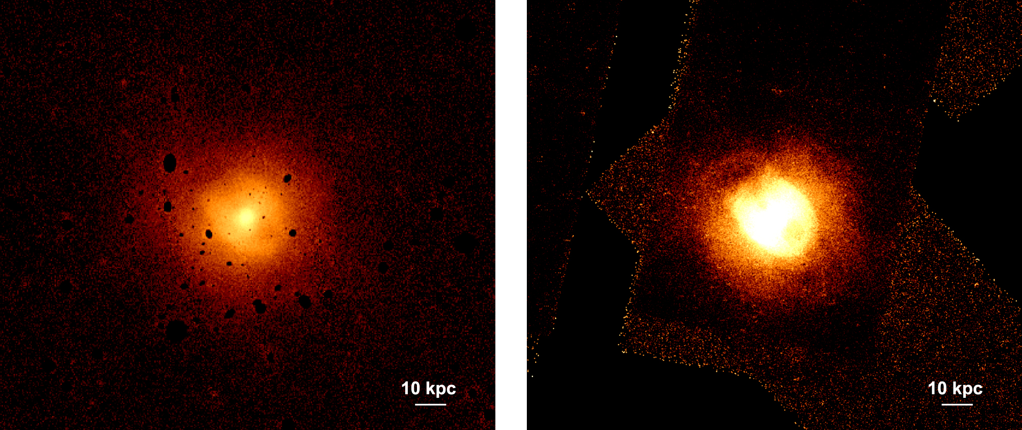
Figure 15. 0.3–3.0 keV surface brightness profile in azimuthal bins across the northern channel of decreased surface brightness shown in Figure 2. The angle Θ is measured from east to north. There is a clear dip at the location of the northern channel, indicating that this is a real feature.
Download figure:
Standard image High-resolution image
Since the northern channel appears to connect to the NE outer cavity, one interesting possibility is that this channel is the result of energy (presumably mostly in the form of non-thermal particles) leaking through the bright cavity rim and heating the ICM. Indeed, the temperature maps shown in Figure 5 show relatively high temperatures in the region of the northern channel, although the correlation between the high-temperature region in the temperature map and the channel in the residual map is not exact. Although cavities are expected to heat the ICM (see Section 6.1), such a direct detection of this heating has not yet been observed. We therefore extracted temperatures both in (wider) azimuthal bins across the northern channel and in identical elliptical regions within and to either side of the channel (at roughly the same distance from the center). In neither case did we find a significant temperature enhancement associated with the channel, with temperatures of all regions agreeing within roughly 1σ. We conclude that, although it is possible that the northern channel is a result of energy leaking from the NE cavity and heating the ICM, causing the gas in this region to expand to pressure equilibrium (and subsequently cool adiabatically) and hence the density (and surface brightness) to drop, we find little evidence to support this interpretation. In particular, we cannot rule out the possibility that this feature is simply due to large-scale structure in the ICM, e.g., associated with previous mergers or bulk motion of the group, even in this relatively relaxed system. Another possibility is that this deficit is a leftover cavity from an even older, fourth outburst that lies off of the axis defined by the other three cavity pairs, although the fact that it is at least partially within the 30 kpc shock front is difficult to reconcile with this interpretation. Deep, low-frequency radio observations would be useful both to detect the putative low-energy non-thermal particles in the NE outer cavity and to see if this emission extends out along the northern channel, consistent with it arising from a leaking cavity.
7. SUMMARY
We have presented results from our analysis of a very deep Chandra observation of the galaxy group N5813. This observation confirms an outer cavity pair and associated shock (only hinted at in R11), giving a total of three pairs of roughly collinear cavities, with each pair associated with an elliptical shock front with a measured temperature jump. The derived Mach numbers are 1.8, 1.5, and 1.2 for the 1, 10, and 30 kpc shocks, respectively. These features are cleanly separated signatures from three distinct outbursts of the central AGN. We compare the shock heating rate to the radiative cooling rate locally at each shock front and find that the rates closely balance one another. This demonstrates that shock heating alone is sufficient to offset gas cooling and enable AGN feedback to operate within at least the central 30 kpc (compared with 10 kpc in R11). We suggest that shock heating is likely important at small radii in other cool core clusters and groups, but that in most cases the shocks are more difficult to detect due to higher ICM temperatures, larger distances, and more complicated ICM structure, or "weather," instigated by mergers. This picture is broadly consistent with results from numerical simulations, which show similar features (weak elliptical shocks, X-ray cavities, etc.) to what we see in N5813 (e.g., Gaspari et al. 2012). We find that the total outburst energies of the old and intermediate-age outbursts are roughly equal, while the energy of the young outburst is more than a factor of 10 less. However, the mean powers of all of the outbursts are roughly the same, within a factor of 2, indicating that the mean kinetic luminosity of the AGN has remained stable for at least 50 Myr. We suggest that the young outburst is ongoing, having deposited only a fraction of its total energy into the ICM. The proximity of the central cavities to the AGN, the relatively high-frequency radio emission that fills the cavities, and the shock-heated rims surrounding the cavities (that have not yet separated from the cavities, as is the case for the older outbursts) are all consistent with this scenario. We find that the 10 kpc (and possibly the 1 kpc) elliptical shock front is broadened by ∼0.4 kpc (∼0.1 kpc), more than 10 times the particle mean free path and thus too broad to be caused by particle diffusion. While we cannot rule out broadening due to a clumpy ICM and/or projection effects, using rough estimates, we find that the measured shock widths (which are upper limits for the 30 kpc shock) are all consistent with broadening due to propagation through a turbulent ICM with a turbulent speed of ∼70 km s−1. This is within, but on the low end of, the range of turbulent speeds expected based on simulations and other observations and thus provides a robust upper limit on the turbulence since other factors may contribute to the total shock broadening. This suggests that transport due to turbulence dominates that of particle diffusion throughout the ICM in N5813. Using spectral fits in the cavity regions, we place lower limits on the temperature of any volume filling gas that could completely balance the pressure within the cavity with that in the external ICM. Our most stringent limit of  keV comes from the intermediate cavity pair. Finally, we find a channel of decreased surface brightness extending north from the outer NE cavity. We suggest that this feature may be due to energy leaking from the cavity and heating the ICM, although we find no temperature enhancement in the channel to support this scenario.
Support for this work was partially provided by the Chandra X-ray Center through NASA contract NAS8-03060, the Smithsonian Institution, and by Chandra X-ray observatory grant GO1-12104X. Basic research in radio astronomy at the Naval Research Laboratory is supported by 6.1 Base funding. We thank A. Foster, R. Smith, H. Russell, and C. Sarazin for useful discussions.