


ABSTRACT
In order to obtain accurate terahertz center frequencies for SO and its isotopologues, we have studied the absorption spectrum of SO, 34SO, and 33SO up to 2.5 THz using continuous-wave terahertz photomixing based on a frequency comb providing an accuracy down to 10 kHz. Sulfur monoxide was produced in a radio frequency discharge of air in a cell containing pure sulfur. Together with the strong absorption signal of the main isotopologue, transitions of 34SO (34S: 4.21%) and 33SO (33S: 0.75%) were observed in natural abundance. The newly observed transitions constitute an extension of the observed rotational quantum numbers of the molecule toward higher N values, allowing an improvement of the molecular parameters for the three species. An isotopically invariant fit has been performed based on pure rotational and ro-vibrational transitions of all SO isotopologues, enabling their accurate line position prediction at higher frequencies. Thanks to this new set of parameters, it is now possible to predict with very high accuracy the frequencies of the ro-vibrational lines. This should enable the research of SO in the mid-IR using ground-based IR telescopes, space-based telescope archives (Infrared Space Observatory, Spitzer), and future space missions such as the James Webb Space Telescope. This set of parameters is particularly well adapted for the detection of SO lines in O-rich evolved stars or in molecular clouds in absorption against bright IR sources.
Export citation and abstract BibTeX RIS
1. INTRODUCTION
Since its first detection in the interstellar medium by means of rotational spectroscopy (Gottlieb & Ball 1973), sulfur monoxide, SO, has been observed in a wide variety of astrophysical environments (see Klaus et al. 1994, and references therein). This transient species is particularly abundant in star-forming regions characterized by high temperature and gas concentrations (Blake et al. 1987). It has been detected in the atmosphere of Venus (Na et al. 1990) and in Io, one of Jupiter's moons, where it is thought to be produced by volcanic and photochemical pathways (Lellouch 1996). In planetary atmospheres, the presence of the SO radical results from the photodecomposition of sulfur dioxide (Krasnopolsky 2012). SO is also an important reaction intermediate in combustion and Earth atmospheric chemistry due to its high reactivity and its role in reactions involving molecules containing nitrogen and oxygen (see Burkholder et al. 1987, and references therein).
SO was first identified in the laboratory in 1932 through the observation of its electronic transitions (Martin 1932). Since then, numerous electronic (Colin 1968), ro-vibrational (Kanamori et al. 1985; Burkholder et al. 1987), as well as pure rotational studies have been dedicated to this radical. The electric dipole moment of SO has also been determined by Stark measurements (1.55 D; Powell & Lide 1964). Pure rotational transitions of SO have been observed in the microwave (Lovas et al. 1992), the terahertz (THz), (Cazzoli et al. 1994), and far infrared (FIR) regions (Cheung et al. 1991; Martin-Drumel et al. 2013) in numerous vibrational states of the ground electronic state (Bogey et al. 1982). SO is also the first molecule for which pure rotational transitions have been detected in several excited electronic states (Saito 1970; Clark & De Lucia 1976; Endo et al. 1987; Bogey et al. 1997; Sanz et al. 2003). Since the sulfur atom possesses three relatively abundant isotopes (32S: 95.02%, 34S: 4.21%, 33S: 0.75%), several studies have also been dedicated to the SO isotopologues (e.g., Tiemann 1982; Klaus et al. 1996; Sanz et al. 2003). Isotopically invariant parameters have been derived from combined fits of all isotopic species (Klaus et al. 1996) and Dunham coefficients have also been determined (Sanz et al. 2003).
Recently, pure rotational transitions of SO have been observed by means of synchrotron-based Fourier-transform FIR (FT-FIR) spectroscopy (Martin-Drumel et al. 2013). In this study, 102 transitions were recorded in the spectral range 1.3–2.8 THz with a frequency accuracy limited to 2 MHz. In the present study, we have re-investigated this range of the spectrum using a photomixing technique allowing a higher accuracy to be achieved (down to 10 kHz). We also have extended the observed transitions of both 34SO and 33SO (detected in natural abundance) toward higher frequencies. Improved effective molecular constants and isotopically invariant parameters have been derived from these new results. Frequency predictions obtained from this new isotopically invariant fit are accurate in the THz region and will permit further exploration of the SO (and its rare isotopologues) spectra in astronomical sources observed with the HIFI instrument (De Graauw et al. 2010) on board the Herschel satellite (Pilbratt et al. 2010; see HEXOS and CHESS Herschel guaranteed programs; Wang et al. 2011; Ceccarelli et al. 2010).
2. EXPERIMENTAL METHOD
The continuous-wave terahertz (cw-THz) photomixing spectrometer used in this study has been described in detail elsewhere (Eliet et al. 2011; Hindle et al. 2011; Mouret et al. 2009). Briefly, the operation of the photomixing source is based on the spatial superposition of two extended cavity diode lasers (ECDLs; emitting around 780 nm) creating an optical beatnote, which is converted to free space THz radiation by a photomixer (ultrafast LTG-GaAs device). This spectrometer is tunable between 0.3 and 3.3 THz. A frequency comb (FC) generated by a frequency doubled erbium doped femtosecond fiber laser enables the achievement of the ECDLs' frequency stability of 1 MHz or better. The FC repetition rate, which separates each mode of the FC, is locked to a low phase-noise oven-controlled crystal oscillator, which is itself locked to the GPS timing signal (Spectracom, EC20S). This reference frequency provides an accuracy of 2 × 10⁻¹² over a period of 24 hr. Two phase-locked loops are used to lock the two ECDLs to the FC, accurately fixing the difference frequency; the accuracy in line frequency is thus only limited by the line profile. The use of a third ECDL ensures a continuous tunability up to 500 MHz, illustrated in the study of the SO radical, wherein a 510 MHz continuous portion of the 32SO spectrum was recorded around 1 THz (Figure 1). This spectrum, showing a rotational triplet, has been recorded in about ten minutes using frequency steps of 400 kHz and a time constant of 100 ms. The periodic variations observed in the baseline of the recordings are caused by a weak Fabry–Perot effect established between the photomixer and the bolometer, here separated by 1.87 m. The photomixing technique has the greatest tuning range of any known coherent source in the THz region, and has a spectral purity smaller than the Doppler limit at room temperature.
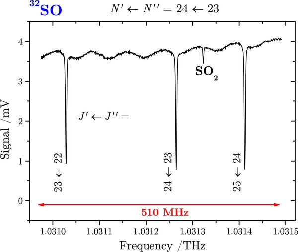
Figure 1. Observation of a fine structure triplet of 32SO over a continuous range of about 500 MHz. This spectrum required about 10 minutes of acquisition time.
Download figure:
Standard image High-resolution imageThe THz beam is collimated through the cell and focused onto a silicon liquid-helium cooled detector by means of two off-axis parabolic mirrors. In this study, both amplitude modulation (AM) and frequency modulation (FM) modes of operation have been used. ΔJ = 1 transitions of 32SO have been recorded in AM using a 263 Hz modulation frequency (Figure 1). ΔJ = 0 transitions of 32SO (100 times weaker than ΔJ = 1) as well as lines of 34SO and 33SO have been recorded in FM with a modulation depth of 120 kHz and a rate of 273 Hz (Figure 2). A second harmonic scheme is employed in order to optimize the signal-to-noise ratio (S/N). Despite this rather slow modulation frequency, which was necessary due to the use of a "slow" Si-bolometer, an improvement in S/N by more than a factor 10 has been observed using the FM instead of the AM configuration.
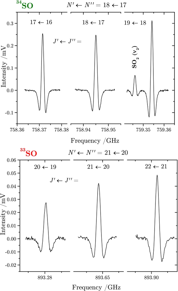
Figure 2. Fine structure triplet of 34SO (upper trace) and 33SO (lower trace) observed in the frequency modulation.
Download figure:
Standard image High-resolution imageThe SO radical was produced by a 50 W radiofrequency discharge using air in a cell containing a pure sulfur deposit. The air flow was ensured by a roughing pump. Absorption levels of up to 80% were obtained for the main isotopologue in its vibrational ground state. 34SO and 33SO isotopologues were observed in natural abundance. A discharge in a flow air and H2S mixture yielded a lower SO concentration. SO2 transitions in the ground and first excited vibrational state have been identified in the spectrum (Figures 1 and 2). Experimental conditions were adjusted for each transition in order to achieve the highest S/N possible in a reasonable acquisition time (pressure: 20–500 μbar; time constant: 0.5–2 s; steps: 100–600 kHz.) S/Ns up to 260, 70, and 40 have been obtained for 32SO, 34SO, and 33SO, respectively.
3. RESULTS AND DISCUSSION
In its fundamental X3Σ− electronic state, SO is an intermediate between Hund's coupling schemes (a) and (b). However, by convention the rotational structure of the radical is described in the (b) formalism using the rotational quantum number N. The coupling between the electronic spin and the rotation of the molecule, by means of spin–spin (interaction between the magnetic moments associated with the two unpaired electrons under the effect of the rotation) and spin–rotation (interaction with Π excited electronic states) coupling, leads to a rotational fine structure of three components (for N > 0) associated with the quantum number J ( , S = 1) and separated by a few hundred GHz (a few wavenumbers).
Due to the wide range of observed frequencies (and thus of FWHMs) and S/Ns, we performed a line profile fit on all transitions to determine their center frequency and estimate their accuracy. Only lines presenting no more than 60% to 70% of absorption (when recorded in AM) were considered in the process to prevent saturating line shapes. Rotational transitions were fitted with a pseudo-Voigt profile of type (1 − s)G + sL (with G and L a Gaussian and Lorentzian function, respectively, and s the "shape" of the line):
where A is the height of the line, B is the center frequency, and C is the FWHM. Compared to a classical Voigt profile, the second derivative of this analytical formula can be easily calculated in order to fit the transitions recorded in FM (second derivative shape). The accuracy of each line position δ(ν) was then estimated from the formula (Landman et al. 1982):
where Δν is the frequency step and S/N is the signal-to-noise ratio.
One-hundred five transitions of 32SO in its vibrational ground state (16 ⩽ N'' ⩽ 58) have been recorded in the spectral region 0.731–2.511 THz with frequency accuracies Δ(ν) ranging from 10 to 800 kHz. 48 (17 ⩽ N'' ⩽ 32) and twenty-one (16 ⩽ N'' ⩽ 22) transitions of the 34SO and 33SO isotopologues in v = 0 have also been observed in natural abundance up to 1.388 THz and 978 GHz, respectively. The observed transitions are presented with their calculated uncertainty in Tables 1–3.
Table 1. Observed Transitions of the 32SO Radical, Uncertainties, and Obs.−Calc. of the Effective Fit (in MHz)
| N' | J' | N'' | J'' | νobs | Unc. | Obs.−Calc. | N' | J' | N'' | J'' | νobs | Unc. | Obs.−Calc. |
|---|---|---|---|---|---|---|---|---|---|---|---|---|---|
| 17 | 16 | 16 | 15 | 730500.794 | 0.006 | 0.003 | 35 | 36 | 34 | 35 | 1500812.597 | 0.052 | 0.011 |
| 17 | 17 | 16 | 16 | 731141.318 | 0.010 | 0.014 | 35 | 35 | 34 | 34 | 1500844.634 | 0.070 | 0.005 |
| 17 | 18 | 16 | 17 | 731596.448 | 0.020 | −0.023 | 36 | 37 | 35 | 36 | 1543337.554 | 0.033 | 0.018 |
| 13 | 13 | 12 | 13 | 735235.258 | 0.443 | −0.134 | 36 | 35 | 35 | 34 | 1543358.014 | 0.030 | −0.015 |
| 18 | 17 | 17 | 16 | 773512.352 | 0.030 | 0.031 | 36 | 36 | 35 | 35 | 1543378.858 | 0.035 | −0.030 |
| 18 | 18 | 17 | 17 | 774064.140 | 0.008 | 0.006 | 37 | 38 | 36 | 37 | 1585833.824 | 0.040 | 0.020 |
| 18 | 19 | 17 | 18 | 774454.646 | 0.020 | −0.021 | 37 | 36 | 36 | 35 | 1585871.743 | 0.039 | −0.015 |
| 14 | 14 | 13 | 14 | 777349.654 | 0.168 | −0.116 | 37 | 37 | 36 | 36 | 1585883.825 | 0.043 | 0.019 |
| 19 | 18 | 18 | 17 | 816495.167 | 0.005 | 0.006 | 38 | 39 | 37 | 38 | 1628300.550 | 0.033 | 0.043 |
| 19 | 19 | 18 | 18 | 816972.307 | 0.008 | −0.001 | 38 | 37 | 37 | 36 | 1628354.537 | 0.030 | −0.054 |
| 19 | 20 | 18 | 19 | 817307.322 | 0.010 | −0.013 | 38 | 38 | 37 | 37 | 1628358.632 | 0.040 | 0.068 |
| 15 | 15 | 14 | 15 | 819582.919 | 0.123 | −0.141 | 41 | 42 | 40 | 41 | 1755514.487 | 0.012 | −0.007 |
| 20 | 19 | 19 | 18 | 859451.295 | 0.020 | 0.020 | 41 | 41 | 40 | 40 | 1755593.648 | 0.060 | −0.063 |
| 20 | 20 | 19 | 19 | 859864.990 | 0.020 | −0.021 | 41 | 40 | 40 | 39 | 1755610.234 | 0.013 | −0.020 |
| 20 | 21 | 19 | 20 | 860152.012 | 0.002 | 0.003 | 42 | 43 | 41 | 42 | 1797854.326 | 0.050 | 0.088 |
| 16 | 16 | 15 | 16 | 861911.759 | 0.233 | −0.018 | 42 | 42 | 41 | 41 | 1797939.761 | 0.111 | 0.104 |
| 21 | 20 | 20 | 19 | 902381.990 | 0.015 | 0.016 | 42 | 41 | 41 | 40 | 1797962.050 | 0.089 | 0.051 |
| 21 | 21 | 20 | 20 | 902741.427 | 0.005 | −0.001 | 43 | 44 | 42 | 43 | 1840160.085 | 0.014 | −0.010 |
| 21 | 22 | 20 | 21 | 902986.581 | 0.005 | 0.001 | 43 | 43 | 42 | 42 | 1840251.568 | 0.210 | 0.213 |
| 22 | 21 | 21 | 20 | 945288.113 | 0.015 | 0.018 | 43 | 42 | 42 | 41 | 1840279.079 | 0.021 | 0.022 |
| 22 | 22 | 21 | 21 | 945600.753 | 0.010 | 0.009 | 44 | 45 | 43 | 44 | 1882431.282 | 0.070 | 0.067 |
| 22 | 23 | 21 | 22 | 945809.191 | 0.010 | −0.012 | 44 | 44 | 43 | 43 | 1882528.012 | 0.030 | 0.025 |
| 23 | 22 | 22 | 21 | 988170.122 | 0.010 | 0.005 | 44 | 43 | 43 | 42 | 1882560.712 | 0.050 | 0.061 |
| 23 | 23 | 22 | 22 | 988442.140 | 0.009 | −0.005 | 45 | 46 | 44 | 45 | 1924666.702 | 0.060 | −0.048 |
| 23 | 24 | 22 | 23 | 988618.234 | 0.005 | −0.008 | 45 | 45 | 44 | 44 | 1924768.576 | 0.124 | −0.156 |
| 24 | 23 | 23 | 22 | 1031028.243 | 0.007 | −0.010 | 45 | 44 | 44 | 43 | 1924805.836 | 0.150 | −0.160 |
| 24 | 24 | 23 | 23 | 1031264.791 | 0.030 | −0.023 | 46 | 47 | 45 | 46 | 1966865.938 | 0.080 | 0.081 |
| 24 | 25 | 23 | 24 | 1031412.184 | 0.015 | −0.029 | 46 | 46 | 45 | 45 | 1966972.835 | 0.037 | 0.061 |
| 25 | 24 | 24 | 23 | 1073862.505 | 0.009 | −0.006 | 46 | 45 | 45 | 44 | 1967014.346 | 0.033 | 0.040 |
| 25 | 25 | 24 | 24 | 1074067.930 | 0.008 | −0.006 | 47 | 48 | 46 | 47 | 2009027.719 | 0.014 | 0.026 |
| 25 | 26 | 24 | 25 | 1074189.757 | 0.005 | −0.002 | 47 | 47 | 46 | 46 | 2009139.291 | 0.057 | −0.001 |
| 26 | 25 | 25 | 24 | 1116672.751 | 0.039 | 0.009 | 47 | 46 | 46 | 45 | 2009184.768 | 0.060 | −0.022 |
| 26 | 26 | 25 | 25 | 1116850.689 | 0.017 | −0.007 | 48 | 49 | 47 | 48 | 2051151.445 | 0.032 | 0.027 |
| 26 | 27 | 25 | 26 | 1116949.615 | 0.010 | −0.001 | 48 | 48 | 47 | 47 | 2051267.430 | 0.085 | −0.036 |
| 28 | 27 | 27 | 26 | 1202220.034 | 0.080 | 0.095 | 48 | 47 | 47 | 46 | 2051316.478 | 0.095 | −0.177 |
| 28 | 28 | 27 | 27 | 1202351.851 | 0.029 | −0.017 | 49 | 50 | 48 | 49 | 2093236.218 | 0.047 | 0.024 |
| 28 | 29 | 27 | 28 | 1202411.573 | 0.026 | −0.016 | 49 | 49 | 48 | 48 | 2093356.472 | 0.038 | −0.006 |
| 29 | 28 | 28 | 27 | 1244956.091 | 0.010 | 0.003 | 49 | 48 | 48 | 47 | 2093409.097 | 0.076 | −0.006 |
| 29 | 29 | 28 | 28 | 1245068.634 | 0.013 | −0.015 | 50 | 51 | 49 | 50 | 2135281.061 | 0.089 | −0.123 |
| 29 | 30 | 28 | 29 | 1245111.501 | 0.011 | −0.003 | 50 | 50 | 49 | 49 | 2135405.481 | 0.114 | −0.027 |
| 30 | 29 | 29 | 28 | 1287666.615 | 0.010 | −0.001 | 50 | 49 | 49 | 48 | 2135461.388 | 0.103 | 0.053 |
| 30 | 30 | 29 | 29 | 1287761.799 | 0.023 | −0.005 | 51 | 52 | 50 | 51 | 2177285.828 | 0.300 | 0.275 |
| 30 | 31 | 29 | 30 | 1287789.321 | 0.024 | 0.007 | 51 | 51 | 50 | 50 | 2177413.796 | 0.084 | 0.061 |
| 31 | 30 | 30 | 29 | 1330351.049 | 0.049 | 0.085 | 51 | 50 | 50 | 49 | 2177472.782 | 0.151 | 0.231 |
| 31 | 31 | 30 | 30 | 1330430.582 | 0.041 | 0.065 | 54 | 55 | 53 | 54 | 2303046.535 | 0.035 | −0.061 |
| 31 | 32 | 30 | 31 | 1330444.057 | 0.038 | 0.040 | 54 | 54 | 53 | 53 | 2303185.285 | 0.063 | −0.111 |
| 32 | 31 | 31 | 30 | 1373008.620 | 0.080 | 0.085 | 54 | 53 | 53 | 52 | 2303252.063 | 0.061 | 0.014 |
| 32 | 32 | 31 | 31 | 1373074.332 | 0.015 | 0.359 | 59 | 60 | 58 | 59 | 2511758.120 | 0.199 | −0.103 |
| 32 | 33 | 31 | 32 | 1373074.332 | 0.015 | −0.306 | 59 | 59 | 58 | 58 | 2511912.066 | 0.165 | −0.094 |
| 33 | 32 | 32 | 31 | 1415638.720 | 0.022 | 0.024 | 59 | 58 | 58 | 57 | 2511988.643 | 0.385 | −0.234 |
| 33 | 34 | 32 | 33 | 1415680.221 | 0.019 | −0.005 | |||||||
| 33 | 33 | 32 | 32 | 1415691.347 | 0.022 | −0.008 | |||||||
| 34 | 33 | 33 | 32 | 1458240.783 | 0.013 | −0.007 | |||||||
| 34 | 35 | 33 | 34 | 1458259.812 | 0.030 | −0.036 | |||||||
| 34 | 34 | 33 | 33 | 1458281.850 | 0.014 | 0.004 |
Download table as: ASCIITypeset image
Table 2. Observed Transitions of the 33SO Radical, Uncertainties, and Obs−Calc. of the Effective Fit (in MHz)
| N' | J' | N'' | J'' | νobs | Unc. | Obs.−Calc. |
|---|---|---|---|---|---|---|
| 17 | 16 | 16 | 15 | 723120.527 | 0.100 | −0.096 |
| 17 | 17 | 16 | 16 | 723773.541 | 0.060 | 0.030 |
| 17 | 18 | 16 | 17 | 724239.271 | 0.100 | 0.115 |
| 18 | 17 | 17 | 16 | 765701.564 | 0.060 | −0.034 |
| 18 | 18 | 17 | 17 | 766264.657 | 0.070 | −0.004 |
| 18 | 19 | 17 | 18 | 766664.898 | 0.050 | 0.029 |
| 19 | 18 | 18 | 17 | 808253.989 | 0.060 | −0.020 |
| 19 | 19 | 18 | 18 | 808741.466 | 0.060 | 0.013 |
| 19 | 20 | 18 | 19 | 809085.500 | 0.030 | 0.036 |
| 20 | 19 | 19 | 18 | 850779.866 | 0.050 | −0.005 |
| 20 | 20 | 19 | 19 | 851203.133 | 0.070 | 0.045 |
| 20 | 21 | 19 | 20 | 851498.467 | 0.050 | −0.008 |
| 21 | 20 | 20 | 19 | 893280.267 | 0.300 | −0.270 |
| 21 | 21 | 20 | 20 | 893648.772 | 0.060 | 0.004 |
| 21 | 22 | 20 | 21 | 893901.769 | 0.070 | −0.024 |
| 22 | 21 | 21 | 20 | 935756.929 | 0.050 | 0.051 |
| 22 | 22 | 21 | 21 | 936077.704 | 0.080 | 0.008 |
| 22 | 23 | 21 | 22 | 936293.460 | 0.100 | −0.120 |
| 23 | 22 | 22 | 21 | 978209.472 | 0.060 | 0.065 |
| 23 | 23 | 22 | 22 | 978489.047 | 0.060 | −0.027 |
| 23 | 24 | 22 | 23 | 978672.033 | 0.130 | −0.171 |
Download table as: ASCIITypeset image
Table 3. Observed Transitions of the 34SO Radical, Uncertainties, and Obs.−Calc. of the Effective Fit (in MHz)
| N' | J' | N'' | J'' | νobs | Unc. | Obs.−Calc. | N' | J' | N'' | J'' | νobs | Unc. | Obs.−Calc. |
|---|---|---|---|---|---|---|---|---|---|---|---|---|---|
| 17 | 16 | 16 | 15 | 716194.548 | 0.011 | −0.006 | 25 | 24 | 24 | 23 | 1052890.648 | 0.016 | −0.002 |
| 17 | 17 | 16 | 16 | 716859.006 | 0.010 | −0.002 | 25 | 25 | 24 | 24 | 1053108.760 | 0.010 | 0.000 |
| 17 | 18 | 16 | 17 | 717334.413 | 0.019 | −0.005 | 25 | 26 | 24 | 25 | 1053242.510 | 0.009 | 0.006 |
| 18 | 17 | 17 | 16 | 758371.481 | 0.005 | −0.009 | 27 | 26 | 26 | 25 | 1136826.278 | 0.017 | 0.003 |
| 18 | 18 | 17 | 17 | 758945.041 | 0.010 | 0.024 | 27 | 27 | 26 | 26 | 1136991.152 | 0.010 | 0.001 |
| 18 | 19 | 17 | 18 | 759354.202 | 0.005 | 0.013 | 27 | 28 | 26 | 27 | 1137080.312 | 0.013 | −0.007 |
| 19 | 18 | 18 | 17 | 800519.976 | 0.005 | 0.001 | 28 | 27 | 27 | 26 | 1178758.414 | 0.019 | −0.018 |
| 19 | 19 | 18 | 18 | 801016.965 | 0.030 | 0.026 | 28 | 28 | 27 | 27 | 1178901.035 | 0.030 | 0.006 |
| 19 | 20 | 18 | 19 | 801369.207 | 0.006 | −0.012 | 28 | 29 | 27 | 28 | 1178971.123 | 0.038 | −0.016 |
| 20 | 19 | 19 | 18 | 842642.090 | 0.012 | 0.023 | 29 | 28 | 28 | 27 | 1220666.290 | 0.032 | 0.001 |
| 20 | 20 | 19 | 19 | 843073.978 | 0.012 | −0.011 | 29 | 29 | 28 | 28 | 1220788.999 | 0.032 | 0.015 |
| 20 | 21 | 19 | 20 | 843377.019 | 0.013 | −0.021 | 29 | 30 | 28 | 29 | 1220841.829 | 0.031 | 0.010 |
| 21 | 20 | 20 | 19 | 884739.175 | 0.011 | 0.019 | 30 | 29 | 29 | 28 | 1262549.397 | 0.023 | 0.001 |
| 21 | 21 | 20 | 20 | 885115.381 | 0.014 | −0.004 | 30 | 30 | 29 | 29 | 1262654.233 | 0.025 | 0.002 |
| 21 | 22 | 20 | 21 | 885375.605 | 0.060 | 0.064 | 30 | 31 | 29 | 30 | 1262691.360 | 0.032 | 0.010 |
| 22 | 21 | 21 | 20 | 926812.158 | 0.010 | 0.010 | 31 | 30 | 30 | 29 | 1304407.197 | 0.024 | −0.031 |
| 22 | 22 | 21 | 21 | 927140.334 | 0.008 | −0.010 | 31 | 31 | 30 | 30 | 1304495.994 | 0.041 | 0.009 |
| 22 | 23 | 21 | 22 | 927362.870 | 0.015 | −0.018 | 31 | 32 | 30 | 31 | 1304518.775 | 0.027 | 0.016 |
| 23 | 22 | 22 | 21 | 968861.590 | 0.011 | 0.007 | 32 | 31 | 31 | 30 | 1346239.181 | 0.055 | −0.043 |
| 23 | 23 | 22 | 22 | 969148.079 | 0.008 | −0.002 | 32 | 32 | 31 | 31 | 1346313.464 | 0.040 | 0.001 |
| 23 | 24 | 22 | 23 | 969337.459 | 0.009 | 0.005 | 32 | 33 | 31 | 32 | 1346323.072 | 0.063 | −0.027 |
| 24 | 23 | 23 | 22 | 1010887.730 | 0.007 | −0.000 | 33 | 32 | 32 | 31 | 1388044.783 | 0.056 | −0.006 |
| 24 | 24 | 23 | 23 | 1011137.816 | 0.008 | 0.001 | 33 | 34 | 32 | 33 | 1388103.506 | 0.062 | 0.059 |
| 24 | 25 | 23 | 24 | 1011297.769 | 0.006 | −0.003 | 33 | 33 | 32 | 32 | 1388105.958 | 0.067 | 0.078 |
Download table as: ASCIITypeset image
The following sections detail the two fitting processes performed in this work. We first performed an effective fit for each of the three isotopologues observed in this study. These fits provide the most accurate rotational parameters for the three molecules. However, due to the lack of predictive reliability of such effective fits (see an example in the next paragraph) we performed a global fit of all the data available on SO (all isotopologues and all vibrational states).
3.1. Effective Fit of 32SO, 34SO, and 33SO
The effective Hamiltonian for SO in its X3Σ electronic ground state is:


where B is the rotational constant, λ the spin–spin coupling constant, and γ the spin–rotation coupling constant, neglecting the centrifugal distortion. In the case of 33SO, the non-null nuclear spin of the 33S (I = 3/2) leads to a hyperfine structure of four components separated by a few tens of MHz. This effect could not be resolved in the present study.
The newly recorded transitions have been fitted using the SPFIT/SPCAT software (Pickett 1991) together with previously available data reported in the literature for 32SO, 33SO and 34SO (see references in Table 4). Multiple experimental values for one transition were kept in the fit (weighted according to their respective accuracy) since they were all obtained by independent measurements. Reduced standard deviations (dimensionless) of 0.88, 0.82, and 0.85 have been obtained for the three fits. Results are compared with Ref. Martin-Drumel et al. (2013) in the case of 32SO, and to a refit of previously available data for the two other isotopologues (Table 5). For each isotopologue, fitting the newly recorded transitions (only), with parameters fixed at their final values, resulted in rms values lower than 100 kHz, and a reduced standard deviation of 0.99, 0.75, and 0.84. This reflects the quality of our measurements and uncertainty estimation.
Table 4. References Used in the Effective and Isotopically Invariant Fits
| Isotopologue | References |
|---|---|
| Effective fit | |
| 32S16O | Powell & Lide (1964); Winnewisser et al. (1964); Amano et al. (1967); Tiemann (1974); Clark & De Lucia (1976); Bogey et al. (1982); |
| Tiemann (1982); Lovas et al. (1992); Cazzoli et al. (1994); Klaus et al. (1996); Bogey et al. (1997); Hansen et al. (1998); | |
| Martin-Drumel et al. (2013); Sanz et al. (2003) | |
| 33S16O | Amano et al. (1967); Klaus et al. (1996); Sanz et al. (2003) |
| 34S16O | Amano et al. (1967); Tiemann (1974); Bogey et al. (1982); Tiemann (1982); Lovas et al. (1992); Klaus et al. (1996); Sanz et al. (2003) |
| Isotopically invariant fit (additional references) | |
| 32S16O | Kawaguchi et al. (1979); Wong et al. (1982); Kanamori et al. (1985); Burkholder et al. (1987) |
| 34S16O | Burkholder et al. (1987); Hansen et al. (1998) |
| 36S16O | Klaus et al. (1996) |
| 32S17O | Klaus et al. (1996) |
| 32S18O | Lovas et al. (1992); Tiemann (1974); Bogey et al. (1982); Tiemann (1982); Klaus et al. (1994, 1996); Burkholder et al. (1987) |
Download table as: ASCIITypeset image
Table 5. Ground State Molecular Constants (in MHz) of 32SO, 33SO, and 34SO, and Comparison with Previous Values
| 32SO | 33SO | 34SO | ||||
|---|---|---|---|---|---|---|
| This Work | Previous Valuesa | This Work | Previous Valuesb | This Work | Previous Valuesc | |
| B | 21 523.555 878 (79) | 21 523.556 16 (37) | 21 306.465 38 (86) | 21 306.465 23 (97) | 21 102.732 28 (31) | 21 102.733 14 (82) |
| D × 103 | 33.915 261 (85) | 33.915 56 (70) | 33.238 7 (11) | 33.239 6 (14) | 32.600 73 (55) | 32 606 4 (13) |
| H × 109 | −6.974 (22) | −7.09 (17) | −6.06 (31) | |||
| λ | 158 254.392 (09) | 158 254.387 (13) | 158 252.22 (14) | 158 252.28 (15) | 158 249.807 (24) | 158 249.816 (27) |
| λD | 0.306 259 (72) | 0.306 53 (20) | 0.303 65 (62) | 0.303 9 (12) | 0.300 63 (08) | 0.300 28 (79) |
| λH × 106 | 0.478 (47) | |||||
| γ | −168.304 3 (15) | −168.304 1 (40) | −166.622 (20) | −166.630 (21) | −164.994 8 (36) | −164.992 9 (65) |
| γD × 103 | −0.525 45 (97) | −0.523 1 (85) | −0.358 (20) | −0.344 (35) | −0.511 6 (27) | −0.515 (22) |
| b | 18.883 (19) | 18.883 (19) | ||||
| c | −96.34 (11) | −96.34 (11) | ||||
| eQq | −15.453 1 (71) | −15.453 1 (71) | ||||
| CI | 0.015 1 (73) | 0.014 8 (74) | ||||
| Fitted lines | 329 | 184 | 100 | 79 | 95 | 48 |
| σd | 0.88 | 0.64 | 0.82 | 0.82 | 0.85 | 0.95 |
Notes. Errors (1σ) are reported in parentheses in the unit of the last digit. aPrevious values from Martin-Drumel et al. (2013). bObtained by refitting data from Amano et al. (1967), Klaus et al. (1996), and Sanz et al. (2003). cObtained by refitting data from Amano et al. (1967), Tiemann (1974), Tiemann (1982), Bogey et al. (1982), Lovas et al. (1992), and Klaus et al. (1996). dReduced standard deviation (dimensionless).
Download table as: ASCIITypeset image
The addition of new transitions with higher N values allows the determination of molecular parameters with higher accuracy. The error of the centrifugal distortion parameters is decreased by up to an order of magnitude. Furthermore, λH for 32SO and H for 34SO have been determined for the first time. In case of 33SO, the hyperfine structure due to the 33S nucleus has not been resolved, hence the hyperfine structure parameters b, c, eQq, and CI are not better determined. The amelioration of the centrifugal distortion parameters is particularly visible when examining the dispersion on the frequency predictions for the 32SO radical in Figure 3. This plot presents the difference between the frequencies of the lines observed in this study (cw-THz) and the calculated frequencies obtained with different parameter sets (obs. − calc.). The experimental uncertainty on the line frequency is plotted as error bars. The calculated frequencies based on the initial set of data (pure rotational data from the literature apart from Martin-Drumel et al. 2013) present the strongest discrepancy with the experimental values. This set of data contains pure rotational transitions up to 1.9 THz and the deviation of the prediction is visible, 2.5 MHz at 2.5 THz, while the error on the frequencies of the lines at 2.5 MHz were estimated to be of only 5 kHz. This illustrates the lack of reliability of effective fits regarding the predictions mentioned above.

Figure 3. Comparison of the frequency predictions of 32SO obtained using the parameters from the initial pure rotation data, those from Martin-Drumel et al. (2013; synchrotron-based FT-FIR), and the final parameters obtained in this study (cw-THz). Error bars are the uncertainty on the frequency of the experimental transitions.
Download figure:
Standard image High-resolution image
We also note that the addition of FT-FIR data in the fit allows a significant improvement of the prediction, despite the fact that these data have a limited frequency accuracy of 2 MHz. This is an illustration of the complementarity of synchrotron-based FT-FIR spectroscopy and cw-THz technique for the study of transient species (see also Martin-Drumel et al. 2012): the former allows a broad survey of the FIR region with a limited resolution (30 MHz), consequently allowing a fast and efficient recording at kHz resolution of the same transitions with the latter technique.
3.2. Isotopically Invariant Fit
In order to provide reliable frequency predictions of SO isotopologues—including rare isotopologues—in the THz range, we performed an isotopically invariant fit. This global fit includes all reported pure rotational and ro-vibrational transitions of SO isotopologues in all observed vibrational states using the fitting programs associated with the MADEX spectroscopic code (Cernicharo 2013). The fitting code was checked against the results of Klaus et al. (1996) and provided the same rotational constants. The Dunham expansions used to determine the matrix elements are those reported in Klaus et al. (1994), although the hyperfine structure has not been considered. For the sake of clarity, energy expressions are summarized below.
The rovibrational energy levels are expressed by an expansion involving the isotopically invariant parameters Uij and the reduced mass μ (in a.u.):

The spin–rotation (SR) and spin–spin (SS) interactions are expressed using the isotopically invariant parameters γij and λij:

The breakdown of the Born–Oppenheimer approximation yields a slight modification of the previous equations. For instance, denoting the isotopes A and B for the two nuclei, the U01 constant is defined as (Tiemann 1982):

where  and
and  carry the corrections to the Born–Oppenheimer approximation. MA and MB are the atomic masses of the considered isotopes while
  and
and  are the atomic masses of the reference isotopes (here 32S and 16O). Atomic masses used in our fits are taken from the AME2012 (Audi et al. 2012; Wang et al. 2012). Unlike the one used by Klaus et al. (1994), our program did not allow us to include hyperfine interactions. Consequently, for isotopologues containing the nuclei 33S (spin I = 3/2) or 17O (spin I = 5/2), the observed hyperfine components have been averaged with a weight relative to their intensities (taken from the CDMS website; Müller et al. 2001), and the resulting frequencies have been included in the global fit.
Pure rotation and ro-vibration transitions of six isotopologues of SO from this work and the literature have been included in our fit. For the first time rotational and vibrational transitions have been merged in an isotopically invariant fit for the SO radical allowing the determination of the Ui0 constants. In total, 1766 transitions were included (see detailed references in Table 4): 1121 for 32S16O with v = 0–33, 53 for 33S16O with v = 0–8, 296 for 34S16O with v = 0–11, 28 for 36S16O with v = 0, 4 for 32S17O with v = 0, and 264 for 32S18O with v = 0–1.
A fit of all rotational and vibrational data using the uncertainties given by the different authors for the IR transitions produces a result in which the uncertainties for the rotational constants, Uij(j ≠ 0), are slightly degraded. An examination of the different sets of IR lines (by looking at the individual reduced standard deviation of each set of data) suggests that the quoted uncertainties for these data are in some cases optimistic. Hence, we have multiplied these uncertainties by a factor of two and eliminated in the final fit all lines for which the observed minus calculated frequencies exceed 3σ. The complete linelist is presented in the machine-readable table. A short example is shown in Table 6. The resulting 43 isotopically invariant parameters are given in Table 7 (reduced standard deviation of the fit: 0.8997). For the sake of comparison with previous studies and to observe the influence of the newly recorded transitions, a global fit including only pure rotational transitions has also been performed. The results are given in column two and can be compared with the results of Klaus et al. (1996) presented in the third column. The uncertainties of all parameters are improved with our data by a factor of 2–5.
Table 6. Pure Rotation and Ro-vibration Transitions of SO Included in the Isotopically Invariant Fit
| Sa | Ob | N' | J' | ν' | N'' | J'' | ν'' | νobs | Unc. | Ref. |
|---|---|---|---|---|---|---|---|---|---|---|
| 1 | 5 | 2 | 1 | 0 | 1 | 1 | 0 | 13043.8 | 0.20 | 1964JCP...41...1413c |
| 1 | 5 | 0 | 1 | 0 | 1 | 0 | 0 | 30001.6 | 0.20 | 1964JCP...41...1413 |
| 1 | 5 | 3 | 2 | 0 | 2 | 2 | 0 | 36201.7 | 0.20 | 1964JCP...41...1413 |
| 1 | 5 | 1 | 2 | 0 | 0 | 1 | 0 | 62931.0 | 0.50 | 1964JCP...41...1413 |
| 1 | 5 | 4 | 3 | 0 | 3 | 3 | 0 | 66034.9 | 0.50 | 1964JCP...41...1413 |
Notes. Positive values indicate frequency in MHz, negative in cm−1. a1 = 32S; 2 = 33S; 3 = 34S; 4 = 36S. b5 = 16O; 6 = 17O; 7 = 18O. cPowell & Lide (1964).
Only a portion of this table is shown here to demonstrate its form and content. A machine-readable version of the full table is available.
Download table as: DataTypeset image
Table 7. Isotopically Invariant Parameters for the SO Radical
| Ro-vibrational | Rotational (This Work) | Rotationala | Units | |
|---|---|---|---|---|
| U10 | 3757.49542(195) | ⋅⋅⋅ | ⋅⋅⋅ | cm−1 |
X |
−0.02551(209) | ⋅⋅⋅ | ⋅⋅⋅ | cm−1 |
X |
−0.017252(516) | ⋅⋅⋅ | ⋅⋅⋅ | cm−1 |
| U20 | −68.32167(622) | ⋅⋅⋅ | ⋅⋅⋅ | cm−1 |
| U30 | 0.47556(818) | ⋅⋅⋅ | ⋅⋅⋅ | cm−1 |
| U40 | −0.04041(463) | ⋅⋅⋅ | ⋅⋅⋅ | cm−1 |
| U50 | 0.005031(934) | ⋅⋅⋅ | ⋅⋅⋅ | cm−1 |
| U01 | 230387.59070(231) | 230387.59057(277) | 230387.56040(520) | MHz amu |
X |
7.80287(568) | 7.80306(679) | 7.8170(230) | MHz amu |
X |
21.4882(454) | 21.4880(542) | 21.5320(270) | MHz amu |
| U11 | −6001.6578(164) | −6001.6561(197) | −6001.4290(360) | MHz amu3/2 |
| U21 | 25.7585(267) | 25.7522(321) | 25.4620(750) | MHz amu2 |
| U31 | −0.8254(175) | −0.8211(211) | −0.5910(560) | MHz amu5/2 |
| U41 | −0.01197(508) | −0.01296(611) | −0.1180(140) | MHz amu3 |
| U51 | −0.022075(633) | −0.021972(759) | ⋅⋅⋅ | MHz amu7/2 |
| U61 | 0.0011700(256) | 0.0011663(306) | ⋅⋅⋅ | MHz amu4 |
| U02 | −3.8543097(229) | −3.8543191(281) | −3.853730(130) | MHz amu2 |
| U12 | −0.004547(114) | −0.004482(144) | −0.008590(390) | MHz amu5/2 |
| U22 | −0.0011636(577) | −0.0011953(717) | ⋅⋅⋅ | MHz amu3 |
| U03 | −0.0000078489(791) | −0.0000078478(946) | −0.00001260(140) | MHz amu3 |
| U13 | 0.0000299(46) | MHz amu7/2 | ||
| U04 | −0.000000001040(146) | −0.000000001041(174) | ⋅⋅⋅ | MHz amu4 |
| γ00 | −1787.4277(276) | −1787.4285(332) | −1787.4230(370) | MHz amu |
| γ10 | −45.508(176) | −45.501(212) | −45.670(210) | MHz amu3/2 |
| γ20 | 1.871(133) | 1.857(160) | 2.210(150) | MHz amu2 |
| γ30 | 0.0986(216) | 0.0995(260) | ⋅⋅⋅ | MHz amu5/2 |
| γ01 | −0.060460(184) | −0.060481(221) | −0.058950(400) | MHz amu2 |
| γ11 | 0.00439(108) | 0.00452(130) | ⋅⋅⋅ | MHz amu5/2 |
| λ00 | 157795.4203(201) | 157795.4208(241) | 157795.5340(680) | MHz |
X |
0.299(229) | 0.303(273) | −0.570(240) | MHz |
X |
−7.722(235) | −7.721(280) | −7.200(130) | MHz |
| λ10 | 2979.597(136) | 2979.592(164) | 2978.670(640) | MHz amu1/2 |
X |
−2.697(160) | −2.702(191) | ⋅⋅⋅ | MHz amu1/2 |
| λ20 | 112.732(159) | 112.745(191) | 114.50(160) | MHz amu |
| λ30 | 13.6225(953) | 13.619(113) | 12.00(130) | MHz amu3/2 |
| λ40 | −0.1057(327) | −0.1054(391) | 0.780(310) | MHz amu2 |
| λ50 | 0.22948(606) | 0.22949(724) | ⋅⋅⋅ | MHz amu5/2 |
| λ60 | −0.018122(580) | −0.018125(692) | ⋅⋅⋅ | MHz amu3 |
| λ70 | 0.0014205(229) | 0.0014203(273) | ⋅⋅⋅ | MHz amu7/2 |
| λ01 | 3.24222(125) | 3.24213(151) | 3.24430(200) | MHz amu |
| λ11 | 0.14226(791) | 0.14287(954) | 0.1490(120) | MHz amu3/2 |
| λ21 | 0.03545(466) | 0.03505(561) | 0.03140(780) | MHz amu2 |
| λ02 | 0.00005374(357) | 0.00005379(426) | ⋅⋅⋅ | MHz amu2 |
| σb | 0.8997 | 0.8112 | 0.70 | |
Notes. Errors (1σ) are reported in parentheses in the unit of the last digit. aConstants derived by Klaus et al. (1996). bReduced standard deviation.
Download table as: ASCIITypeset image
Born–Oppenheimer Breakdown (BOB) coefficients have been derived from the isotopically invariant fit following the formula (for an atom A; Watson 1980):

Table 8 presents these coefficients together with a comparison with Klaus et al. (1996). Δ01 coefficients are slightly better determined while Δ10 are determined for the first time.
Table 8. Born–Oppenheimer Breakdown (BOB) Coefficients Derived from the Isotopically Invariant Fit
| Parameter | This Work | Klaus et al. (1996) |
|---|---|---|
 |
−1.9725 (14) | −1.9772 (58) |
 |
−2.7175 (57) | −2.7247 (34) |
 |
0.395 (32) | ⋅⋅⋅ |
 |
0.1338 (40) | ⋅⋅⋅ |
Note. Errors (1σ) are reported in parentheses in the unit of the last digit.
Download table as: ASCIITypeset image
Finally, molecular parameters for 12 isotopologues of SO in v = 0 to 5 (32S16O, 32S17O, 32S18O, 33S16O, 33S17O, 33S18O, 34S16O, 34S17O, 34S18O, 36S16O, 36S17O, 36S18O) have been derived from the isotopically invariant fit using a nonlinear least squares method. The obtained parameters are presented in Tables 9–12. The quality of the determination of the obtained parameters can be estimated since the error is dominated by the one of the dominant parameters (Y01 for B0, Y02 for D0, Y03 for H0,...). As an example, for 32SO in v = 0 the error on B0 (21 523.556 51 MHz, Table 9) should be of the order of 2 kHz (i.e., the error on Y01; Table 7) for all isotopologues, which is the strength of the isotopically invariant fit. This can be verified by comparison with the B0 value obtained using the effective fit for 32SO (21 523.555 878 (79) MHz; Table 5). The two values differ by 0.6 kHz, attesting to the quality of the derived parameters. However, for 32SO, 33SO, and 34SO in their vibrational ground state, the rotational constants of Table 5 are more accurate. For all other isotopologues and vibrational states, the parameters given in the previous tables will permit the prediction of reliable rotational frequencies in the THz domain.
Table 9. Derived Parameters (in MHz) for 32SO in the Six Lowest Vibrational Levels of the Electronic Ground State
| v = 0 | v = 1 | v = 2 | v = 3 | v = 4 | v = 5 | |
|---|---|---|---|---|---|---|
| Isotopologue 32S16O | ||||||
| B | 21523.55651 | 21351.59505 | 21180.06610 | 21008.95451 | 20838.24344 | 20667.91389 |
| D × 102 | 3.39162 | 3.39304 | 3.39465 | 3.39645 | 3.39845 | 3.40063 |
| H × 109 | −6.47734 | −6.47734 | −6.47734 | −6.47734 | −6.47734 | −6.47734 |
| L × 1014 | −8.04693 | −8.04693 | −8.04693 | −8.04693 | −8.04693 | −8.04693 |
| γ | −168.30517 | −169.57865 | −170.81684 | −172.01815 | −173.18097 | −174.30370 |
| γD × 104 | −5.26007 | −5.14161 | −5.02315 | −4.90469 | −4.78623 | −4.66777 |
| λ | 158254.38332 | 159189.34399 | 160148.99572 | 161135.78421 | 162152.28832 | 163201.27051 |
| λD × 101 | 3.06232 | 3.10943 | 3.16278 | 3.22236 | 3.28818 | 3.36023 |
| λH × 107 | 4.73466 | 4.73466 | 4.73466 | 4.73466 | 4.73466 | 4.73466 |
| Isotopologue 32S17O | ||||||
| B | 20677.80911 | 20515.89547 | 20354.38135 | 20193.25309 | 20032.49559 | 19872.09182 |
| D × 102 | 3.12977 | 3.13105 | 3.13250 | 3.13412 | 3.13591 | 3.13787 |
| H × 109 | −5.74192 | −5.74192 | −5.74192 | −5.74192 | −5.74192 | −5.74192 |
| L × 1014 | −6.85242 | −6.85242 | −6.85242 | −6.85242 | −6.85242 | −6.85242 |
| γ | −161.66569 | −162.86535 | −164.03249 | −165.16566 | −166.26342 | −167.32432 |
| γD × 104 | −4.85508 | −4.74793 | −4.64079 | −4.53365 | −4.42651 | −4.31937 |
| λ | 158244.74695 | 159160.65402 | 160100.21102 | 161065.71645 | 162059.58924 | 163084.41473 |
| λD × 101 | 2.94132 | 2.98556 | 3.03555 | 3.09130 | 3.15281 | 3.22006 |
| λH × 107 | 4.36914 | 4.36914 | 4.36914 | 4.36914 | 4.36914 | 4.36914 |
| Isotopologue 32S18O | ||||||
| B | 19929.27880 | 19776.08755 | 19623.26769 | 19470.80683 | 19318.69126 | 19166.90561 |
| D × 102 | 2.90683 | 2.90799 | 2.90930 | 2.91077 | 2.91239 | 2.91416 |
| H × 109 | −5.13947 | −5.13947 | −5.13947 | −5.13947 | −5.13947 | −5.13947 |
| L × 1014 | −5.91098 | −5.91098 | −5.91098 | −5.91098 | −5.91098 | −5.91098 |
| γ | −155.79078 | −156.92631 | −158.03168 | −159.10556 | −160.14663 | −161.15358 |
| γD × 104 | −4.51015 | −4.41246 | −4.31478 | −4.21709 | −4.11940 | −4.02171 |
| λ | 158236.06300 | 159134.79727 | 160056.26376 | 161002.63355 | 161976.18753 | 162979.35856 |
| λD × 101 | 2.83426 | 2.87602 | 2.92312 | 2.97556 | 3.03335 | 3.09648 |
| λH × 107 | 4.05792 | 4.05792 | 4.05792 | 4.05792 | 4.05792 | 4.05792 |
Notes. Weighted sigma = 0.6791. Standard deviation = 8.8978 MHz.
Download table as: ASCIITypeset image
Table 10. Derived Parameters (in MHz) for 33SO in the Six Lowest Vibrational Levels of the Electronic Ground State
| v = 0 | v = 1 | v = 2 | v = 3 | v = 4 | v = 5 | |
|---|---|---|---|---|---|---|
| Isotopologue 33S16O | ||||||
| B | 21306.46510 | 21137.10196 | 20968.16273 | 20799.63267 | 20631.49538 | 20463.73240 |
| D × 102 | 3.32341 | 3.32479 | 3.32635 | 3.32811 | 3.33005 | 3.33217 |
| H × 109 | −6.28291 | −6.28291 | −6.28291 | −6.28291 | −6.28291 | −6.28291 |
| L × 1014 | −7.72650 | −7.72650 | −7.72650 | −7.72650 | −7.72650 | −7.72650 |
| γ | −166.60082 | −167.85522 | −169.07505 | −170.25875 | −171.40477 | −172.51154 |
| γD × 104 | −5.15457 | −5.03908 | −4.92359 | −4.80810 | −4.69261 | −4.57712 |
| λ | 158252.04078 | 159182.12015 | 160136.62293 | 161117.95670 | 162128.65888 | 163171.44597 |
| λD × 101 | 3.03126 | 3.07763 | 3.13011 | 3.18869 | 3.25339 | 3.32420 |
| λH × 107 | 4.63944 | 4.63944 | 4.63944 | 4.63944 | 4.63944 | 4.63944 |
| Isotopologue 33S17O | ||||||
| B | 20460.68961 | 20301.32252 | 20142.34669 | 19983.74883 | 19825.51426 | 19667.62643 |
| D × 102 | 3.06426 | 3.06550 | 3.06691 | 3.06848 | 3.07022 | 3.07213 |
| H × 109 | −5.56258 | −5.56258 | −5.56258 | −5.56258 | −5.56258 | −5.56258 |
| L × 1014 | −6.56855 | −6.56855 | −6.56855 | −6.56855 | −6.56855 | −6.56855 |
| γ | −159.96154 | −161.14248 | −162.29159 | −163.40747 | −164.48870 | −165.53387 |
| γD × 104 | −4.75372 | −4.64938 | −4.54503 | −4.44069 | −4.33634 | −4.23199 |
| λ | 158242.35753 | 159153.28989 | 160087.60564 | 161047.56603 | 162035.54963 | 163054.09712 |
| λD × 101 | 2.91026 | 2.95378 | 3.00293 | 3.05771 | 3.11812 | 3.18417 |
| λH × 107 | 4.27769 | 4.27769 | 4.27769 | 4.27769 | 4.27769 | 4.27769 |
| Isotopologue 33S18O | ||||||
| B | 19712.13399 | 19561.44258 | 19411.11459 | 19261.13798 | 19111.49943 | 18962.18404 |
| D × 102 | 2.84370 | 2.84483 | 2.84611 | 2.84753 | 2.84911 | 2.85083 |
| H × 109 | −4.97297 | −4.97297 | −4.97297 | −4.97297 | −4.97297 | −4.97297 |
| L × 1014 | −5.65704 | −5.65704 | −5.65704 | −5.65704 | −5.65704 | −5.65704 |
| γ | −154.08680 | −155.20395 | −156.29159 | −157.34845 | −158.37325 | −159.36469 |
| γD × 104 | −4.41247 | −4.31743 | −4.22238 | −4.12734 | −4.03229 | −3.93725 |
| λ | 158233.62960 | 159127.30151 | 160043.44012 | 160984.18000 | 161951.76266 | 162948.57746 |
| λD × 101 | 2.80321 | 2.84426 | 2.89053 | 2.94203 | 2.99876 | 3.06072 |
| λH × 107 | 3.96980 | 3.96980 | 3.96980 | 3.96980 | 3.96980 | 3.96980 |
Notes. rms = 8.8978 MHz. Reduced standard deviation = 0.6791.
Download table as: ASCIITypeset image
Table 11. Derived Parameters (in MHz) for 34SO Isotopologues in the Six Lowest Vibrational Levels of the Electronic Ground State
| v = 0 | v = 1 | v = 2 | v = 3 | v = 4 | v = 5 | |
|---|---|---|---|---|---|---|
| Isotopologue 34S16O | ||||||
| B | 21102.73177 | 20935.79500 | 20769.27415 | 20603.15484 | 20437.42111 | 20272.05496 |
| D × 102 | 3.26002 | 3.26137 | 3.26289 | 3.26460 | 3.26649 | 3.26856 |
| H × 109 | −6.10403 | −6.10403 | −6.10403 | −6.10403 | −6.10403 | −6.10403 |
| L × 1014 | −7.43459 | −7.43459 | −7.43459 | −7.43459 | −7.43459 | −7.43459 |
| γ | −165.00144 | −166.23801 | −167.44069 | −168.60794 | −169.73826 | −170.83011 |
| γD × 104 | −5.05654 | −4.94379 | −4.83105 | −4.71831 | −4.60556 | −4.49282 |
| λ | 158249.83181 | 159175.30919 | 160124.95906 | 161101.15343 | 162106.39109 | 163143.34570 |
| λD × 101 | 3.00211 | 3.04778 | 3.09945 | 3.15712 | 3.22077 | 3.29042 |
| λH × 107 | 4.55095 | 4.55095 | 4.55095 | 4.55095 | 4.55095 | 4.55095 |
| Isotopologue 34S17O | ||||||
| B | 20256.92979 | 20099.94025 | 19943.33428 | 19787.09895 | 19631.21996 | 19475.68122 |
| D × 102 | 3.00340 | 3.00462 | 3.00599 | 3.00752 | 3.00921 | 3.01107 |
| H × 109 | −5.39771 | −5.39771 | −5.39771 | −5.39771 | −5.39771 | −5.39771 |
| L × 1014 | −6.31026 | −6.31026 | −6.31026 | −6.31026 | −6.31026 | −6.31026 |
| γ | −158.36234 | −159.52580 | −160.65808 | −161.75780 | −162.82358 | −163.85406 |
| γD × 104 | −4.65958 | −4.55782 | −4.45605 | −4.35429 | −4.25253 | −4.15077 |
| λ | 158240.10389 | 159146.34526 | 160075.72015 | 161030.45505 | 162012.89091 | 163025.52682 |
| λD × 101 | 2.88112 | 2.92396 | 2.97232 | 3.02620 | 3.08560 | 3.15052 |
| λH × 107 | 4.19274 | 4.19274 | 4.19274 | 4.19274 | 4.19274 | 4.19274 |
| Isotopologue 34S18O | ||||||
| B | 19508.35030 | 19359.99236 | 19211.99045 | 19064.33282 | 18917.00655 | 18769.99714 |
| D × 102 | 2.78509 | 2.78619 | 2.78743 | 2.78882 | 2.79035 | 2.79202 |
| H × 109 | −4.82003 | −4.82003 | −4.82003 | −4.82003 | −4.82003 | −4.82003 |
| L × 1014 | −5.42626 | −5.42626 | −5.42626 | −5.42626 | −5.42626 | −5.42626 |
| γ | −152.48777 | −153.58775 | −154.65885 | −155.69981 | −156.70939 | −157.68634 |
| γD × 104 | −4.32177 | −4.22917 | −4.13657 | −4.04397 | −3.95136 | −3.85876 |
| λ | 158231.33403 | 159120.23139 | 160031.34651 | 160966.77998 | 161928.73653 | 162919.56506 |
| λD × 101 | 2.77408 | 2.81446 | 2.85996 | 2.91058 | 2.96633 | 3.02719 |
| λH × 107 | 3.88798 | 3.88798 | 3.88798 | 3.88798 | 3.88798 | 3.88798 |
Notes. rms = 8.8978 MHz. Reduced standard deviation = 0.6791.
Download table as: ASCIITypeset image
Table 12. Derived Parameters (in MHz) for36SO in the Six Lowest Vibrational Levels of the Electronic Ground State
| v = 0 | v = 1 | v = 2 | v = 3 | v = 4 | v = 5 | |
|---|---|---|---|---|---|---|
| Isotopologue 36S16O | ||||||
| B | 20727.98664 | 20565.48218 | 20403.37916 | 20241.66385 | 20080.32103 | 19919.33356 |
| D × 102 | 3.14502 | 3.14631 | 3.14777 | 3.14940 | 3.15120 | 3.15317 |
| H × 109 | −5.78394 | −5.78394 | −5.78394 | −5.78394 | −5.78394 | −5.78394 |
| L × 1014 | −6.91936 | −6.91936 | −6.91936 | −6.91936 | −6.91936 | −6.91936 |
| γ | −162.05980 | −163.26380 | −164.43512 | −165.57230 | −166.67389 | −167.73844 |
| γD × 104 | −4.87867 | −4.77087 | −4.66308 | −4.55528 | −4.44749 | −4.33969 |
| λ | 158245.74142 | 159162.69970 | 160103.36959 | 161070.05823 | 162065.19394 | 163091.37241 |
| λD × 101 | 2.94850 | 2.99291 | 3.04310 | 3.09908 | 3.16083 | 3.22837 |
| λH × 107 | 4.39043 | 4.39043 | 4.39043 | 4.39043 | 4.39043 | 4.39043 |
| Isotopologue 36S17O | ||||||
| B | 19882.13562 | 19729.48795 | 19577.20994 | 19425.28926 | 19273.71231 | 19122.46379 |
| D × 102 | 2.89307 | 2.89423 | 2.89553 | 2.89699 | 2.89860 | 2.90036 |
| H × 109 | −5.10303 | −5.10303 | −5.10303 | −5.10303 | −5.10303 | −5.10303 |
| L × 1014 | −5.85516 | −5.85516 | −5.85516 | −5.85516 | −5.85516 | −5.85516 |
| γ | −155.42104 | −156.55257 | −157.65409 | −158.72427 | −159.76181 | −160.76539 |
| γD × 104 | −4.48887 | −4.39176 | −4.29464 | −4.19753 | −4.10042 | −4.00331 |
| λ | 158235.92958 | 159133.48463 | 160053.71427 | 160998.78163 | 161970.95902 | 162972.66986 |
| λD × 101 | 2.82752 | 2.86913 | 2.91605 | 2.96829 | 3.02584 | 3.08872 |
| λH × 107 | 4.03872 | 4.03872 | 4.03872 | 4.03872 | 4.03872 | 4.03872 |
| Isotopologue 36S18O | ||||||
| B | 19133.51192 | 18989.41421 | 18845.65911 | 18702.23545 | 18559.13096 | 18416.33189 |
| D × 102 | 2.67888 | 2.67992 | 2.68111 | 2.68242 | 2.68387 | 2.68546 |
| H × 109 | −4.54697 | −4.54697 | −4.54697 | −4.54697 | −4.54697 | −4.54697 |
| L × 1014 | −5.02030 | −5.02030 | −5.02030 | −5.02030 | −5.02030 | −5.02030 |
| γ | −149.54677 | −150.61541 | −151.65628 | −152.66820 | −153.64997 | −154.60040 |
| γD × 104 | −4.15740 | −4.06919 | −3.98098 | −3.89277 | −3.80456 | −3.71635 |
| λ | 158227.08088 | 159107.13481 | 160008.94931 | 160934.56297 | 161886.11354 | 162865.87626 |
| λD × 101 | 2.72049 | 2.75966 | 2.80376 | 2.85279 | 2.90674 | 2.96561 |
| λH × 107 | 3.73972 | 3.73972 | 3.73972 | 3.73972 | 3.73972 | 3.73972 |
Notes. rms = 8.8978 MHz. Reduced standard deviation = 0.6791.
Download table as: ASCIITypeset image
4. CONCLUSION
New pure rotational transitions of the SO radical and of its two most abundant isotopologues have been measured in the THz spectral region (up to 2.5 THz). The use of the cw-THz photomixing technique based on a FC allowed very high accuracy line frequency measurements. Reliable effective parameters have been obtained for these three isotopologues. We also performed a global mass independent fit including all pure rotational and ro-vibrational transitions reported in the literature on all observed isotopologues of SO.
Thanks to this new set of parameters it is now possible to predict with very high accuracy the frequencies of the ro-vibrational lines. This should enable the research of SO in the mid-IR using ground-based IR telescopes, space-based telescope archives (Infrared Space Observatory, Spitzer), and future space missions such as the James Webb Space Telescope. This set of parameters particularly well-adapted for the detection of SO lines in O-rich evolved stars or in molecular clouds in absorption against bright IR sources.
The authors gratefully acknowledge Caroline C. Womack for her helpful comments on the manuscript. The THz spectrometer was funded by the Communauté urbaine de Dunkerque, the Région Nord-Pas de Calais, the Ministére de l'éducation nationale, de l'enseignement supérieur et de la recherche, and European funds in the context of the IRENI (Institut de Recherche en ENvironnement Industriel) and InterregIVA "Cleantech" programs. J. Cernicharo thanks the Spanish MINECO program for funding support through grants CSD2009-00038 (CONSOLIDER program "ASTROMOL"), AYA2009-07304, and AYA2012-32032, and the European Research Council for funding under the European Union's Seventh Framework Program (FP/2007-2013) / ERC-2013-SyG, Grant Agreement No. 610256 NANOCOSMOS.