


ABSTRACT
We show the importance of γ and positron transport for the formation of late-time spectra in Type Ia supernovae (SNe Ia). The goal is to study the imprint of magnetic fields (B) on late-time IR line profiles, particularly the [Fe ii] feature at 1.644 μm, which becomes prominent two to three months after the explosion. As a benchmark, we use the explosion of a Chandrasekhar mass (MCh) white dwarf (WD) and, specifically, a delayed detonation model that can reproduce the light curves and spectra for a Branch-normal SN Ia. We assume WDs with initial magnetic surface fields between 1 and 109 G. We discuss large-scale dipole and small-scale magnetic fields. We show that positron transport effects must be taken into account for the interpretation of emission features starting at about one to two years after maximum light, depending on the size of B. The [Fe ii] line profile and its evolution with time can be understood in terms of the overall energy input by radioactive decay and the transition from a γ-ray to a positron-dominated regime. We find that the [Fe ii] line at 1.644 μm can be used to analyze the overall chemical and density structure of the exploding WD up to day 200 without considering B. At later times, positron transport and magnetic field effects become important. After about day 300, the line profile allows one to probe the size of the B-field. The profile becomes sensitive to the morphology of B at about day 500. In the presence of a large-scale dipole field, a broad line is produced in MCh mass explosions that may appear flat-topped or rounded depending on the inclination at which the SN is observed. Small or no directional dependence of the spectra is found for small-scale B. We note that narrow-line profiles require central 56Ni as shown in our previous studies. Persistent broad-line, flat-topped profiles require high-density burning, which is the signature of a WD close to MCh. Good time coverage is required to separate the effects of optical depth, the size and morphology of B, and the aspect angle of the observer. The spectra require a resolution of about 500 km s−1 and a signal-to-noise ratio of about 20%. Two other strong near-IR spectral features at about 1.5 and 1.8 μm are used to demonstrate the importance of line blending, which may invalidate a kinematic interpretation of emission lines. Flat-topped line profiles between 300 and 400 days have been observed and reported in the literature. They lend support for MCh mass explosions in at least some cases and require magnetic fields equal to or in excess of 106 G. We briefly discuss the effects of the size and morphology of B on light curves, as well as limitations. We argue that line profiles are a more direct measurement of B than light curves because they measure both the distribution of 56Ni and the redistribution of the energy input by positrons rather than the total energy input. Finally, we discuss possible mechanisms for the formation of high B-fields and the limitations of our analysis.
Export citation and abstract BibTeX RIS
1. INTRODUCTION
Type Ia supernovae (SNe Ia) are invaluable for probing the large-scale structure of the universe and the origin of the elements. They also provide important laboratories for the study of the physics of flames, instabilities, radiation transport, non-equilibrium systems, and nuclear and high-energy physics. The consensus picture is that SNe Ia result from a degenerate C/O white dwarf (WD) undergoing a thermonuclear runaway (Hoyle & Fowler 1960), and that these in turn originate from close binary stellar systems. Potential progenitor systems may consist of two WDs, a so-called double degenerate system (DD), and/or a single WD and a main-sequence, helium, or red giant star, called a single degenerate system (SD). Candidate progenitor systems have been observed for both the SD and DD cases (Greiner et al. 1991; van den Heuvel et al. 1992; Rappaport et al. 1994; Kahabka & van den Heuvel 1997; Ruiz-Lapuente et al. 2004; González Hernández et al. 2009; Kerzendorf et al. 2009; Schaefer & Pagnotta 2012; Edwards et al. 2012). For recent overviews, see proceedings of the IAU 281 Symposium edited by DiStephano & Orio (2012).
Within this general picture for progenitors, two classes of explosion scenarios have been discussed, which are distinguished by the triggering mechanism of the thermonuclear explosion. The first is the dynamical merging of two C/O WDs in a binary system. In this scenario, the thermonuclear explosion is triggered by the heat of the merging process. However, it is unclear whether the dynamical merging process leads to an SN Ia, an "accretion-induced collapse," or a WD with a high magnetic field. Another problem is that there seem to be too few potential progenitor systems (Webbink 1984; Iben & Tutukov 1984; Benz et al. 1990; Rasio & Shapiro 1994; Hoeflich & Khokhlov 1996; Segretain et al. 1997; Yoon et al. 2007; Wang et al. 2009b, 2009a; Pakmor et al. 2011; Lorén-Aguilar et al. 2009; Isern et al. 2011).
The second scenario involves the explosion of a C/O WD with a mass close to the Chandrasekhar limit (MCh). The explosion in this scenario is triggered by compressional heating near the WD center. Because the compressional heat released increases rapidly as the star nears MCh, the exploding stars are in a very narrow mass range (Hoeflich & Khokhlov 1996). The donor star may be either a red giant or main-sequence star of less than seven to eight solar masses or a helium star in an SD system (Whelan & Iben 1973), or the accreted material may originate from a tidally disrupted WD in a DD system (Whelan & Iben 1973; Piersanti et al. 2003).
A comprehensive discussion of the progenitors and explosion mechanisms is beyond the scope of this paper. For reviews and different views, see (Branch & Miller 1993; Pakmor et al. 2011; Calder et al. 2013; Guidry & Messer 2013; Hoeflich et al. 2013). Theoretical work and observational constraints from the spectra and light curves (LCs) favor the SD scenario for the majority of cases, with some contribution from the DD scenario (Hoeflich & Khokhlov 1996; Saio & Nomoto 1998; Woosley & Weaver 1986; Mochkovitch & Livio 1990; Saio & Nomoto 1985; Quimby et al. 2006; Shen et al. 2011; Hoeflich et al. 2013). Within MCh mass explosions, delayed-detonation models (Khokhlov 1991; Woosley & Weaver 1994; Yamaoka et al. 1992; Gamezo et al. 2003; Gamezo et al. 2005; Poludnenko et al. 2011), in which the burning front transitions from the deflagration to a detonation regime, have been found to reproduce the optical and infrared LCs and spectra of individual "typical" SNe Ia reasonably well, including the time evolution (Hoeflich 1995; Hoeflich & Khokhlov 1996; Fisher et al. 1997; Nugent 1997; Wheeler et al. 1998; Lentz et al. 2001; Marion et al. 2009; Maund et al. 2010; Sim et al. 2013; Dessart et al. 2014) and statistical properties, such as the small spread in the brightness-decline relation (Hoeflich et al. 1996; Nugent et al. 1997; Hoeflich et al. 2002; Maeda et al. 2003; Kasen et al. 2009; Baron et al. 2012). The overall spherical structure in SN Ia remnants and, in particular, the layered chemical structure observed in S-Andromeda are clear evidence of a detonation phase (Fesen et al. 2007). Though small, deviations from sphericity are to be expected owing to rotation of the WD, off-center DDT, and turbulence in the deflagration phase. These have been shown to be present in studies of spectropolarization, IR line profiles, and SN remnants (Howell et al. 2001; Hoeflich et al. 2004; Motohara et al. 2006; Hoeflich et al. 2006; Gerardy et al. 2007; Fesen et al. 2007; Maund et al. 2010; Fesen et al. 2007; Maeda et al. 2011). Recently, correlations between line profiles and LCs (Maeda et al. 2011) and line profiles and polarization (Maund et al. 2010) promise further progress toward a more complete picture of SNe Ia.
We regard four properties of SNe Ia as the primary evidence in favor of MCh explosions: a tight relation of the absolute brightness with the rate of the decline in brightness, low continuum polarization (Wang et al. 1997; Howell et al. 2001; Patat et al. 2012), evidence for nuclear burning at densities >109 g cm−3 from late-time IR spectra (Hoeflich et al. 2004; Motohara et al. 2006; Maeda et al. 2011), and narrow Ni lines at late times as observed in SN 2003hv (Gerardy et al. 2007). In SN 2003hv, late-time mid-IR (MIR) spectra at about 130 days have been obtained with the Spitzer Space Telescope. They show flat-top profiles consistent with the near-IR (NIR) profile and thus support the kinematic interpretation. Whereas the forbidden Co lines are broadly consistent with the expected distribution of 56Ni, late-time Ni lines are found to be narrow. Since 56Ni has a decay time of about 6.3 days, after several months only stable Ni isotopes are left, and they exist only in the central region (Gerardy et al. 2007; Stritzinger et al. 2014). Thus, at least some SNe originate from MCh mass explosion.
Despite the success of MCh mass explosions, whether they originate from SD or DD systems, there are serious problems within this picture related to the mixing by Rayleigh–Taylor (R-T) instabilities inherent in current multidimensional simulations of deflagration fronts (Khokhlov 1995; Niemeyer & Hillebrandt 1995; Livne 1999; Reinecke et al. 1999; Gamezo et al. 2003; Plewa 2007; Röpke et al. 2006). During the deflagration phase, the unburned material is heated by the diffusion of energy from the burned ashes to the unburned fuel. R-T instabilities increase the surface area of the burning front and thus control the rate of burning while mixing the burning products of different layers. Although a layered chemical structure is partially restored during the detonation phase (Gamezo et al. 2005; Röpke et al. 2012), all current three-dimensional (3D) models for the explosions predict R-T mixing of iron-group plumes into the outer layers and mixing of the inner layers, both of which are at odds with observations.
To understand the inconsistencies, it is necessary to both probe the distribution of radioactive material in SNe Ia and look for new physical effects not considered in current 3D simulations for deflagration fronts. Late-time line profiles of [Fe ii] and [Co iii] probe the distribution (Hoeflich et al. 2004; Motohara et al. 2006; Maeda et al. 2011) and provide evidence for high magnetic fields in excess of 3000 G (Hoeflich et al. 2004; Sadler 2012), a piece of physics that may influence the runaway and burning instabilities (see below). Moreover, advances in observational techniques have allowed measurement of spectra at late times and thus are providing an increasingly comprehensive set of SN Ia data (Phillips 2012; Stritzinger et al. 2014).
The distribution of elements and the strength and structure of B may be a key to a better understanding of SNe Ia. However, depending on the phase, a direct translation of the Doppler shifts of a spectral feature is limited by optical depth effects, line blending, and a mix of geometrical asymmetries in the distribution. Moreover, a quantification of the B-fields requires detailed gamma and positron transport. Past studies of line profiles were based on the assumption of local energy deposition of positrons.
The goal of this work is to present a systematic study of the effect of B-fields on the NIR line features. We use a spherical density and chemical distributions and base our study on a DDT model as reference. We employ detailed Monte Carlo schemes for the transport for photons, gamma rays, and positrons. In Section 2 we present a new positron transport scheme and briefly summarize the other tools employed for the simulations. In the following sections, the results are presented and discussed. We present a systematic study of the evolution of NIR profiles of [Fe ii] and [Co iii] in the 1.6–1.7 μm region. We show the importance of time sequences to untangle the various effects.
2. METHODS
Our analysis of the line profiles is based on the delayed detonation model 5p0z00.25, a Branch-normal SN Ia that is part of the series published by Hoeflich et al. (2002). As in our previous analysis of the NIR [Fe ii] line (Hoeflich et al. 2004), the 3D transport is calculated using a Monte Carlo scheme implemented in HYDRA, which includes detailed γ-ray transport. Forbidden lines are included from databases published by Kurucz (1993, 2002), Nussbaumer & Storey (1988b), Nussbaumer & Storey (1988a), Liu et al. (1997a), and Bowers et al. (1997). The new addition here involves the energy deposition by positrons and the extension from γ to X-rays. These new modules will be described in the following.
2.1. Positron Transport Scheme
Several previous investigators have studied the transport of energy by high-energy photons through SN envelopes (Ambwani & Sutherland 1988; Burrows & The 1990; Chan & Lingenfelter 1991; Hoeflich et al. 1994; Hoeflich 2002). As part of his PhD thesis, Penney (2011) implemented new bound–free and bound–bound transitions that allow us to calculate X-ray spectra. This transport module has been further extended to incorporate positron transport in the presence of magnetic fields.
Several authors have addressed the transport of positrons (Bussard et al. 1979; Brown & Leventhal 1987). Early studies by Colgate et al. (1980) and Chan & Lingenfelter (1993) used one-dimensional approximations and assumed that the magnetic field was either chaotically twisted at a scale small enough to trap the positrons in place or radially combed by the expansion, restricting the positrons to move radially. They calculated the energy deposition by positrons at late times and demonstrated the extent to which positron escape would lead to LCs declining faster than the rates of the radioactive decay driving them. Milne et al. (1999) presented calculations using cross sections and a Monte Carlo technique more similar to ours, but continued to use either a radial magnetic field or ones that are chaotic and sufficiently large to trap all positrons. As part of the thesis of Penney (2011), LC results have been compared to those published Milne et al. (2004). As discussed below, we found a generally good agreement, but with a slightly reduced positron escape. In this paper, we make use of line profiles to measure positron transport effects and their dependency on B. Profiles can be expected to be more sensitive and cleaner than LCs because they measure directly the change in the redistribution function of the energy deposition from radioactive decay. In contrast, LCs rely on one quantity, the total energy deposition in the envelope that powers the bolometric LC. The reconstruction of the bolometric LC depends, in turn, on the photon redistribution in frequency space, and after a few years, other energy sources may become important, such as interaction between the SN and the interstellar material.
2.2. Positron Creation and Cross Sections
The primary source of positrons is the β+ channel of the 56Co → 56Fe*, which accounts for about 18% of all 56Co decays. About 1.4 MeV of the total excitation energy of 56Fe* is available to be split between neutrinos and positrons, with the resulting positron energy spectrum (Nadyozhin 1994) given by

where C is a scale factor and η is the charge of the nucleus times ℏ over the velocity of the electron. The mean energy of the spectrum is 0.632 MeV.
A small number of relatively high energy positrons are also contributed by pair production from the high-energy gamma-ray lines of 56Co decay. As most γ rays escape without interaction at late times, these contribute only a few percent to the total positron production by 300 days, but their production and transport are included. The cross section for this channel of positron production has been discussed by Ambwani & Sutherland (1988b).
For the Monte Carlo transport, we take into account three dominant processes of interaction: scattering off atomic electrons as the positron moves through the media, the similar excitation of free electrons in a plasma, and direct annihilation with electrons.
The annihilation cross section is given by Equation (2) (Lang 1999):
where ro = e2/mc2 and γ is the Lorentz factor. In undergoing this interaction, the positron is destroyed, its kinetic energy is deposited into the surrounding material, and its rest-mass energy is released as gamma rays.
Following Chan & Lingenfelter (1993) and Gould (1971), the energy loss by interaction with charged particles is given by

Π(γ) is a relativistic correction given by

where q is the relative charge of the particles in the media. For atomic electron interactions, q is the atomic number Z for the atom. For plasma scattering, q is the ionization fraction. Parameter bmax is the maximum impact parameter, equivalent to the maximum amount of energy the positron can lose in one interaction. For atomic electron scattering, it is the ionization potential. Since the dependence on this parameter is weak, we simplify by using an average ionization potential for the medium. For the case of interactions with electrons in the plasma, the maximum impact parameter is ℏω because the impact with a free electron sets up a disturbance in the plasma that has an energy proportional to the frequency. Note that the ionization stage depends on time and requires ionization models that, in turn, will depend on the energy deposition by positrons. In this study, we assume single ionization. Other sources of continuous energy loss, those of bremsstrahlung and synchrotron radiation, were considered but found to be minor contributions and, for computational efficiency, have been omitted in this study.
The relative strengths of the three types of cross sections are shown in Figure 1. Annihilation is a very small part of the cross section throughout most of the energy range of the positron spectrum. As the positrons scatter and continuously lose energy, though, they will either fall into the range where direct annihilation dominates and be destroyed or slow down until their energies become similar to the binding energy of atomic electrons, form positronium, and be annihilated.

Figure 1. Strength of the electron, plasma, and annihilation cross sections for a single ionized plasma. Annihilation dominates at low energies after the positrons lose most of their energy by electron and plasma interaction. Electrons dominate plasma interactions for low ionization levels, but ions will dominate in highly ionized plasmas.
Download figure:
Standard image High-resolution imageBetween 1 keV and the binding energy of nearby electrons, the positron can undergo charge exchange, stripping an electron off nearby atoms to form positronium, which has a negligible lifetime before undergoing either e+e− → 2γ or e+e− → 3γ for para- and ortho-positronium, respectively. We assume that the para-state and ortho-state of positronium are in statistical equilibrium for the creation of γ photons. The cross section of this process for elements other then H is not well known but is generally proportional to the Bohr radius and thus much larger than the direct annihilation cross section.
This uncertainty in the cross section for annihilation at low energies will hardly influence the location of the energy deposition because the energy loss is large (see Equation (3)). Even at day 1000 after the explosion, the range of a 1 keV positron is less than 0.1% of the radius of the envelope. Thus, we assume that once a positron has fallen below 1 keV, it deposits its kinetic energy locally and annihilates via positronium formation. Chan & Lingenfelter (1993) found that some small fraction of thermalized positrons (≈0.1% in models similar to ours) will avoid annihilation, surviving as "slow" positrons as the envelope density becomes low enough for the lifetime before positronium formation to become very long. However, these positrons will have already deposited their kinetic energy in the ejecta, and their mass energy would not contribute to the low energy light curves and spectra whether they eventually annihilate or not. At late times, γ rays from annihilation are almost guaranteed to escape the envelope without interaction.
2.3. Positron Transport
The transport is solved via a Monte Carlo method very similar to the photon transport (Hoeflich et al. 1994; Hoeflich 2002). A background model is discretized, and the radiation transport is performed in individual computational cells. Upon interaction, the process is chosen randomly, weighted by the size of the individual cross sections.
The motion of positrons depends on the presence, size, and morphology of the magnetic field B imposing a Lorentz force on the positron. The positron is gyrating around the magnetic field line. The scale imposed by B is the Larmor radius

The significance of the gyro motion depends on the size of rL relative to the scale of variations of the explosion model rM, such as the density scale height or the scale of the B-field changes.
For computational efficiency, we distinguish three different implementations: (1) rL ≫ rM, (2) rL ≪ rM, and (3) the case in between.
In Case 3, the path of the positron must be explicitly integrated by breaking the path length into segments sufficiently small so that the B-field changes little along individual segments. A positron propagates along a circular arc on that path (the radius determined by Equation (5)) until it is absorbed, scatters, or escapes the envelope.
Cases 1 and 2 avoid the need to reconstruct the path for individual positrons; thus, they allow for a higher computational efficiency by a factor of more than ≈10.
For Case 1, small magnetic fields, the path of the positron is nearly straight and we integrate along linear rays until the positron is absorbed, is scattered, or escapes.
For large magnetic fields, rL is small compared to the structure of the explosion model. The positron can be assumed to follow the field line on a spiral trajectory mean-free path. The general motion of a positron is along the field line with its path length increased by a factor of 1/sin (θp), where θp is the pitch angle the positrons momentum vector makes with the field line. Effects of gradients in B are implemented following Chen (2003). We divide these into two forces, one parallel to the field lines and one perpendicular. The former causes the "magnetic mirror" effect. Because the first adiabatic invariant is constant, a change in the B-field strength along the direction of travel causes a change in the pitch angle. In the code, we average the derivative of the B-field over the zone in the direction of the field lines and use this to calculate an average gyro-radius for that zone. The result is that positron diffusion is discouraged in the direction of increasing magnetic field and encouraged in the opposite direction, as an increasing pitch angle will increase the path length. The effect of the perpendicular component of the B gradient forces the mean positron path to not follow the field line due to gradients perpendicular to the B-field. We add this velocity to the motion of the particle in each zone using the following equation:
For illustration, Table 1 shows the evolution of rL for a typical SN Ia model as a function of time. In practice, we use Case 3 or Case 1 if rL is smaller than the resolution of the background model or larger than twice the model grid, respectively. Cases 1 and 3 have been tested against the general Case 2. With time and lower magnetic fields, the range of the positron transport increases. For B-fields larger than 109 G, positrons follow the field lines. For B-fields less than 103 G and about 1 year, the bending of the path of the positrons remains small and they travel along rays. We note that turbulence will produce structures of about 1%–5% of the envelope structure. Thus, the energy deposition by positrons requires full transport of positrons for all B-fields less than B ≈ 106 G when the transport effects are important.
Table 1. Maximum Larmor Radius as a Fraction of the Radius of the Supernova Envelope at Various Times and Initial Surface Field Strengths
| Field/Time | 20 days | 60 days | 100 days | 300 days | 500 days |
|---|---|---|---|---|---|
| 103 G | .38 | 1.15 | 1.9 | 5.7 | 9.6 |
| 104 G | .03 | .11 | .19 | .57 | .96 |
| 106 G | .003 | .001 | .001 | .005 | .009 |
| 109 G | 3E − 6 | 1.1E − 6 | 1.9E − 6 | 5E − 6 | 9E − 6 |
Notes. Here, the radius is defined as the layer expanding with a velocity of 40,000 km s−1. Typically, turbulent velocities in the progenitor and during the deflagration phase of burning are between ≈200 and ≈1000 km s−1 (Hoeflich & Stein 2002; Gamezo et al. 2005), or 5 × 10⁻³ and 2.5 × 10⁻² in units of the fractions given.
Download table as: ASCIITypeset image
3. THE REFERENCE MODEL
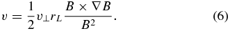
This study uses a spherical, delayed detonation model as a reference model. This model has been successful in reproducing the optical and IR LCs and spectra of a branch-normal SN Ia, 5p0z22.25 (Hoeflich et al. 2002). The C/O WD originates from a progenitor with a main-sequence mass of 5 M☉ and solar metallicity. At the time of the explosion, the central density of the WD was 2 × 10⁹ g cm−3, and the transition from deflagration to detonation was triggered at a density of 25 × 106 g cm−3. About 0.6 M☉ of 56Ni is produced. The density, velocity, and chemical structure are given in Figure 2. As typical for MCh mass explosions, the high-density burning in the central region produced stable isotopes of iron-group elements rather than radioactive 56Ni. Spherical models suppress mixing by R-T instabilities; as a consequence, we produce a central hole in the 56Ni distribution of about 3000 km s−1. The spherical explosion model and evolution have been calculated using 912 radial zones in the comoving frame. Positron transport is inherently 3D in the presence of B-fields. For the γ and positron and NIR transport, the model has been remapped into the observers frame using a Euclidian grid with 330 radial zones with a resolution of about 50 km s−1 up to the Si-rich layers. For θ and ϕ, we use 70 zones with equidistant spacing in sin θ and ϕ. The energy deposition has been stored on a Cartesian grid of 5013 with a matching resolution of 100 km s−1. The emitted photons have been detected in 21 counters each in both θ and ϕ, and about 2500 counters in frequency/energy. The averaged positron spectrum is detected in 100 counters. A typical run uses a package of (1–5) × 1010 photons and positrons.
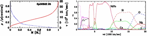
Figure 2. Structure of a spherical delayed detonation model that can reproduce LCs and spectra of Branch-normal SNe Ia (Hoeflich et al. 2002). Density (blue, dotted) and velocity (red, solid) as a function of the mass are given on the left. Abundances of the most abundant stable isotopes as a function of the expansion velocity are given on the right. In the center, the abundances correspond to 54Fe, 58Ni, and Co. We note that current 3D calculations predict similar density structures but with strong chemical mixing.
Download figure:
Standard image High-resolution imageTo study the effects of B, we imprint various fields onto the model described above. We assume that the initial field prior to the explosion of the WD can be described as a dipole with a surface-averaged field of B. For the rotation, we assume that the WD is a rigid rotator with angular velocity w and a constant magnetization m. Taking the field due to a thin spherical shell and summing to the radius of the dwarf Ro (taking R to be the radius of the WD at 90% of the Chandrasekhar mass, 1600 km), the structure of the field is given by

B-field strengths are considered between 1 and 109 G. With the surface field as a boundary condition, we use Equation (7) to calculate the magnetic field throughout the progenitor. Note that the maximal range of the field strength is larger by about a factor of four close to the center of the initial WD. We can assume that the magnetic field is frozen into the matter during the explosion. The final structure of the field is very similar because of the similarity of the initial structure and the homologous expansion of the WD. After the initial acceleration phase, a few minutes into the expansion, the time evolution of the field at every point decreases as the square of the radius and thus with time because of conservation of the magnetic flux. During the homologous expansion, field strength at r is given by Bo(ro/r)2.
4. RESULTS
In this section, we discuss the use of IR lines as a tool for studying the underlying chemical structure and the signature of the strength and structure of the magnetic fields at late times. The use of LCs is also considered briefly and compared to that of IR lines. Both LCs and spectral line profiles allow the probing of magnetic fields. The advantage of broadband LCs is that they provide high photon statistics. This allows one to obtain accurate LCs until very late times and, in principle, for a large number of objects. However, late-time LCs contain limited information because they mostly depend on one quantity only: the combined escape probability of γ rays and positrons. Spectra contain information about the escape probability and the time-dependent redistribution functions, but limiting photon statistics puts high demands on the observations and limits their use to local SNe. Both the resulting LCs and spectra can be understood in terms of the energy deposition.
4.1. Energy Deposition by X-Rays, γ Rays, and Positrons
Radioactive decay of 56Ni → 56Co → 56Fe is the dominant energy source that powers the LCs and spectra of SNe Ia. The total energy input depends on the total mass of the initial 56Ni and the redistribution by transport effects. 56Ni decays by electron capture, which leads to the emission of high-energy photons when the excited 56Co transitions to its ground state. Besides decay via electron capture, 18% of all decays of 56Co are β+ and lead to the emission of a positron.
Escape Probabilities: First, we want to discuss the role of the escape probabilities and their implications for LCs (Figure 3). The small cross sections for γ rays result in rapidly increasing escape fractions. Already at maximum light, ≈20 days after the explosion, 15% of all γ rays escape. This fraction increases to about 85% and 98% by day 100 and day 300, respectively. In contrast, the large positron cross sections cause almost complete local annihilation of positrons up to about 200 days. The length of the positron path depends on the size of B, which causes a strong dependence of the positron escape fraction on B at later times. However, as the kinetic energy of positrons only accounts for some 3% of the total energy produced by 56Co decay, the total energy input is dominated by γ rays until around days 150–200 (Figure 3). Thus, studying the B-field via the influence of energy deposition on optical/IR wavelengths inherently requires late-time observations.
Figure 3. Escape probability for photons and positrons (left) and contribution to the total energy input in % (right) as functions of time. Magnetic fields influence positron transport only. Probing magnetic fields requires late-time observations.
Download figure:
Standard image High-resolution imageLight Curves: Previously, detailed simulations for positron transport effects on the bolometric LCs have been published by (Milne et al. 1999) for a wide range of models based on the deflagration model W7 (Nomoto 1984), the delayed-detonation models (Yamaoka et al. 1992; Hoeflich & Khokhlov 1996; Hoeflich et al. 1998), helium detonations (Ruiz-Lapuente et al. 1993; Hoeflich & Khokhlov 1996), and pulsating-delayed detonation and merger models (Hoeflich et al. 1995; Hoeflich & Khokhlov 1996). We have compared the energy escape by positrons of our reference model and dipole fields with model DD23C (Hoeflich et al. 1998) and radial magnetic fields used in the sample of Milne et al. (1999). We find that our escape fractions agree with Milne et al. (1999) within ≈20%. For high B-fields, our escape fractions are slightly smaller because we include nonradial fields whereas Milne et al. (1999) consider the radial component only.
For a brief discussion, we use the V band (V) as a proxy for the bolometric LC (Arnett 1980). LCs are shown in Figure 4 for low and high B for dipole and turbulent fields. The scale of the turbulent field has been taken to be one pressure scale height in the progenitor WD. The formation of early-time optical and IR LCs has been previously discussed (Hoeflich et al. 1998; Hoeflich et al. 2002; Dessart et al. 2014).

Figure 4. Influence of the size and morphology of B on the visual LCs for our reference model. V is given for dipole and turbulent fields.
Download figure:
Standard image High-resolution imageBetween 60 and 200 days, the decay of V is steeper than is expected from the decay of 56Co because γ-ray photons dominate the energy input and they rapidly increase their escape probability, as shown in Figure 3. In fact, this discrepancy caused early predictions that SNe Ia are not powered by 56Ni (Colgate et al. 1962). Note that the decline rate increases at about 100–200 days with decreasing brightness because more centrally concentrated 56Ni causes a delay in the γ escape (Hoeflich et al. 1993, 2002).
After 300 days, almost all γ rays escape and the LC is dominated by positrons. As the envelope is now optically thin for optical photons, the anisotropy effects are expected to be small. At ≈300 days, V closely mimics the decay curve of cobalt. The change of slope after this point may be used to estimate B (Milne et al. 1999). At about 300 days, the influence of B remains small, ≈0.05 mag. After about 3 yr, the influence of B grows to about 1 mag. Even for high B, the path of positrons follows the magnetic field line, allowing some positron mobility and, then, positron escape. In contrast, for a turbulent field photons are trapped, which results in local energy deposition (see Figure 4) until the field weakens to the point that the Larmor radius is larger than the size of the turbulence. Despite the significance of both the size and morphology of the B-field on late-time bolometric LCs, there are several limitations in using LCs to probe B. Monochromatic LCs are needed to reconstruct bolometric LC. However, V or UBVRI may not actually represent the bolometric LCs. It has been suggested that emission will shift from the V band to the infrared as the timescales of atomic transitions in the optical range increase relative to those in the infrared owing to falling matter densities (called the IR catastrophe). In models, the IR catastrophe may set in anywhere from 300 to 400 days depending on the details of the atomic model and data and the abundances (Fransson et al. 1996). Moreover, recent observations of SNe Ia identified MIR emission lines as a major cooler starting at about three to four months after the explosion (Gerardy et al. 2007; Li et al. 2014). Finally, other energy sources may contribute to the energetics, such as interaction of the envelope with its surroundings, which will deposit energy in the high-velocity layers. Moreover, the diversity among SNe Ia has been well established, and variations in the 56Ni distributions will change the bolometric LCs. These uncertainties and variables make it difficult to extract B-field strengths from just the one quantity provided by LCs.
The Energy Distribution: We want to shift our discussion to the distribution of the energy deposition and the resulting line profiles. The energy depositions by γ rays and positrons and by positrons only are given in Figure 5. Up to about 100–200 days, the contribution from positrons is locally deposited owing to high cross sections. Nonlocality is produced by γ rays. At early times, about a week after the explosion, the optical depth for γ rays is still large and the energy input closely traces the distribution of the radioactive isotopes (Figure 2). We can see the "hole" in the center occupied by stable, electron capture elements. Owing to geometrical dilution, the optical depth for γ photons decreases with time (t) as ≈t−2. This leads to an increasing energy deposition in the central region and larger heating of the outer layers. By about 100 days, the central heating peaks. With time, positrons take over as the main contributors to the energy deposition, and a central hole reappears.
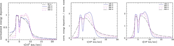
Figure 5. Energy input  per gram and second by both γ rays and positrons assuming local trapping (left), and angle-averaged by positrons for initial magnetic fields of B = 1 G (middle) and 109 G (left), respectively. We normalized the total
  to v ≈ 4000 km s−1 to compare the overall distributions and to compensate for the rapid decrease of trapped energy by γ rays (see Figure 3).
  of positrons has been normalized to the average over the entire envelope.
Download figure:
Standard image High-resolution imageWe start with the case of positron transport without B. Trapping can be attributed to the opacities only as the positron travels along a ray. The escape fractions and the normalized total and positron energy redistribution functions are given in Figures 3 and 5. Up to about 100 days, positrons continue to be locally confined. At 200 days, the outer layers are transparent, diffuse enough that the positrons escape, lowering the amount of high-velocity material that is heated, but positrons in the inner layers remain locally confined. At 300 days small features like the dip in Ni at 5000 km s−1 are starting to be washed out, and there is some penetration into the core. Note that dip in 56Ni is not physical, but an artifact of spherical DDT. However, it is a good indicator to what degree positron transport has become nonlocal. After 500 days, the nonradiating core and the area around it are the only parts of the envelope dense enough to have almost complete positron capture. At 300 to about 400 days, the total energy deposition is at a minimum at the center and subsequently increases as a result of the growing mean free path of positrons.
Magnetic fields determine the path of positrons and thus introduce three more parameters into our discussion: the size of the field, its morphology, and the orientation of the B-field relative to an observer. The main effect of the B-field on the escape and energy redistribution can be understood in terms of the Larmor radius rL compared to the size of the envelope and any substructures considered. It increases the effective mean free path and influences the direction.
For dipole fields, we see that high magnetic fields delay the overall evolution of the energy distribution by about 1 year. For example, the distribution at 200 days resembles closely that of the high B-field at day 500 (Figure 5).
From the previous sections and within the delayed detonation scenario, we can conclude the following: up to about 200–300 days, the energy deposition functions do not depend on magnetic fields because γ-ray transport dominates or positrons are deposited locally regardless of the field. Subsequently, positron transport effects may become important, depending on B.
4.2. NIR Line Profiles for Dipole Fields
The goal of this section is to demonstrate the signature of radiation and positron transport on late-time spectra. We discuss in detail the 1.644 μm spectral feature, including its evolution with time and its dependence on the orientation of the observer. In addition, adjoining strong NIR features are considered to demonstrate the impact of line blending and how blending may severely limit a kinematic interpretation of profiles. For the spectral band, we have calculated a full grid of 30 models for B = 100, 3, 4, 6, 9 G at 100, 200, 300, 400, 500, 999 days with counters in five and eight directions in the Eulerian Θ and ϕ coordinates. Here, we show only a few of the resulting 1200 spectra.
Our reference model, though spherical, requires full 3D transport because of the axial symmetry introduced by the magnetic field. Chemical abundances take into account the variability caused by the radioactive decay 56Ni → 56Co → 56Fe. The excitation balance has been calculated using our non-LTE code (Hoeflich et al. 2004) as a function of time. For the ionization, we found a mean ionization of about 1–1.5 electrons per atom and have assumed a value of 1.5. We neglect second-order effects on the excitation and ionization, although the ionization in the central regions will depend on the heating by positrons and, at late times, iron-group elements may be neutral. As discussed in the final section, this approximation can be tested by observations but can be justified as follows: Lower ionization means a slightly larger mean free path, by about 20%–30% (Figure 1). However, a larger mean free path implies more heating, which, in turn, decreases positron transport (see Section 2), which, in turn, reduces the feedback effect. Tests have shown that the total effect on the spectral features remains small.
To discuss line profiles, the continuum fluxes have been subtracted and the maximum fluxes normalized. The actual abundances have been used from the model 5p0z22.25. For the spectral synthesis, we included the forbidden line profiles of [Fe ii] at 1.533, 1.560, 1.644, 1.664, 1.677, 1.712, 1.745 μm and [Co iii] at 1.55, 1.74, 1.76 μm. The continuum flux in the 1.6–1.7 μm band is 0.24, 0.15, 0.12, 0.1, 0.06, and 0.02 at 100, 200, 300, 400, 500, and 999 days, respectively.
The evolution with time is shown in Figure 6 in velocity space corresponding to wavelengths between 1.5 and 1.8 μm. There are three prominent features at about −20, 000, 0, and +18, 000 km s−1.
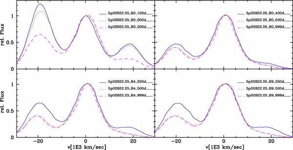
Figure 6. Evolution of the NIR for B = 1 and 104, 9 G is shown in the upper and lower panels, respectively. The continuum flux has been subtracted and the flux normalized to the peak of the 1.644 μm feature. The spectra are labeled by  , where A identifies the model, b = log (B), and C is the time after the explosion in days. T = 1, 5, and 3 denotes observation from polar and equatorial direction, respectively, and
  indicates angle averaging.
Download figure:
Standard image High-resolution imageLow Magnetic Fields: We start with a discussion of the angle-averaged line profile of [Fe ii] at 0 km s−1 ≡ 1.644 μm because line-blending effects for this feature remain small except in the wings (Hoeflich et al. 2004). By day 100, the profile is peaked because gamma rays are nonlocal and mostly absorbed in the central, high-density region, which has stable 54Fe. The [Fe ii] feature is asymmetric and blueshifted by about 2000 km s−1 because the photosphere blocks the redshifted layers of the envelope. By day 200, the blueshift is reduced to about ≈800 km s−1. With time, the feature becomes wider and reaches a maximum width at about 300 days. At around the same time, it develops a flat-top or stumpy appearance in the center. As discussed and shown in Section 5, a caustic profile is produced if 56Ni is homogeneously mixed to the center or the explosion of a low-density WD because the emission would follow the density structure (Hoeflich et al. 2004). By about day 200, positron transport results in increasingly wider line wings and a small low-velocity emission component. By day 500, positrons are able to enter and deposit their energy in the core, and the profile becomes increasingly peaked.
Role of Magnetic Fields: Magnetic fields will hardly change line profiles up to about a year after the explosion. At about 300 days, the envelope is mostly optically thin in the quasi-continuum. Observations of the profile of [Fe ii] at 1.644 μm at this time provide an excellent tool to measure the distribution of 56Ni in the velocity space. Earlier, optical depth effects in the continuum and the contribution of γ rays are important contributors to the energy input. Later, positrons transport energy into the central regions, and at a rate dependent not just on the 56Ni distribution and density structure, but also on the magnitude and structure of the B-field. In practice, early variability in the profiles allows us to separate optical depth and geometry effects, to probe the distribution of the central nonradioactive Fe, and to test for ionization effects.
To detect the effects of B, we want to focus on the Late-time evolution (Figure 7). With increasing B, the evolution from flat-topped or stubby to more centrally peaked profiles is delayed by about 1 year for high B-fields, as can be expected from the discussion above. Lines are narrower by about 20% by day 500 compared to models with B > 106 G. Observations at about 1000 days would allow the measurement of ≈109 G.
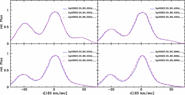
Figure 7. Influence of the size of the B-field on line profiles at 300, 400, 500, and 999 days. For the labeling scheme, see Figure 6.
Download figure:
Standard image High-resolution imagePerils of Line Blending: The kinematic interpretation of emission features breaks down if line blending becomes important, as is the case for features in the optical and most features in the NIR. The two features neighboring the 1.644 μm line, at −20, 000 and +18, 000 kms−1 in Figure 6, are illustrations of the perils of apparently clean features. In fact, they are blends. The former feature is produced by transitions of [Fe ii] at 1.533 and 1.560 μm and of [Co iii] at 1.55 μm. The latter feature is produced by transitions of [Fe ii] at 1.712 and 1.745 μm and of [Co iii] at 1.74 and 1.76 μm.
The evolution of both these satellite features is dominated by the decay of radioactive 56Co. Up to about day 200, the forbidden 56Co lines are responsible for most of the emission. After about day 300, only 56Fe is left, as evidenced also by the slowly varying line ratio between the 1.644 μm feature and the satellites.
Early on, the red feature at +18, 000 km s−1 shows a blueshift similar to [Fe ii] at 1.644 μm but it is broader because several line transitions contribute including [Fe ii] at 1.712 and 1.745 μm and [Co iii] at 1.74 and 1.76 μm. One may expect that, with time, the feature would be shifted toward the blue because of the longer wavelength of the [Co iii] transitions. However, we see a redshift because the feature formed on the wing of the 1.644 μm, which produces a sloped quasi-continuum.
The −20, 000 km s−1 feature at ≈1.55 μm dominates the NIR spectra early on. However, owing to its nature, a simple interpretation may be misleading. With time, this feature undergoes a blueshift opposite to the behavior of the [Fe ii] at 1.644 μm. Taking at face value and in a kinematic interpretation, this would mean that we see an offset in 56Ni, whereas this shift, at least in the models, is due to the changing importance of [Co iii] versus [Fe ii].
In summary, time evolution allows us to detect and, potentially, to separate line blending, geometry, and B-field effects. The [Fe ii] feature at 1.644 μ is rather unique in the NIR.
Directional Dependence of NIR Features: Large-scale magnetic dipole fields introduce a directional dependence of the observed line profile. The variations in the profiles can be understood in terms of the Larmor radius given in Table 1. We consider only times later than 300 days when positron transport effects may be significant. For low B-fields, the Larmor radius is much larger than the envelope and positrons travel on rays, which results in isotropic profiles.
In Figures 8, 9 and 10, the directional dependence of profiles is shown for high magnetic fields. For B = 109 G, the positrons follow the field lines with an increase in the effective cross section. Variations in the energy deposition and, thus, the energy deposition depend mainly on the mean free path. By day 1000, positrons created in the polar regions can travel to the center regardless of the B-field. More generally, positrons created at more equatorial latitudes are funneled toward the pole. This geometry effect causes maximum directional dependence. From the pole, we see flat-topped profiles with an increased line width. Seen from the equator, late-time profiles are centrally peaked.
Figure 8. Directional dependence of the spectrum of the reference model as a function of the Doppler shift relative to the forbidden [Fe ii] at 1.644 μm, assuming a dipole field of 104 G. The solid, dotted, and dashed lines correspond to Θ of 0  , 90
, 90  , and 180
  , respectively. The panels show the spectra at 300, 400, 500, and 999 days after the explosion.
Download figure:
Standard image High-resolution image
Figure 9. Same as Figure. 8, but for B = 106 G.
Download figure:
Standard image High-resolution image
Figure 10. Same as Figure. 8, but for B = 109 G.
Download figure:
Standard image High-resolution imageLowering the B-field increases the mean free path, and the path of the positron is bent but does not exactly follow the field lines. For B = 106 G, the directional dependence shows up earlier. High-precision observations of the time dependence of profiles would allow us to learn about the orientation of the field relative to the observer.
4.3. Influence of the Morphology of the Magnetic Field
This leads us to the effects of the morphology of the B-fields. We may expect a dipole field in a WD prior to the runaway, but it may be distorted by the turbulent motion during the thermonuclear runaway, or by RT instabilities during the explosion of the WD.
As an example and limiting case, we have calculated the transport for a turbulent field. In calculations of the thermonuclear runaway, the largest turbulent eddies are ≈5% of the WD (Hoeflich & Stein 2002). We note that the energy deposition is close to isotropic.
The results are dominated by the change of the gyro-radius relative to the size of the structure of the B-field (Table 1). B in excess of 106 G results in local trapping of positrons with some transport effects starting at about 500–1000 days. For fields less than ≈104 G, the gyro-radius is much larger than the size of the envelope and, consequently, the results are identical to the angle-averaged profiles in Figures 6 and 7. Probing the magnetic fields requires time series of profiles after about two to three years, or magnetic fields between 104 and 106 G observed beyond 400 days. As discussed above for very high magnetic fields, LCs come close to the case of full trapping.
5. DISCUSSION AND CONCLUSIONS
We have presented a new implementation of positron transport using a Monte Carlo method. This allows us to study the transport effects in full 3D for arbitrary magnetic fields without the need for either the low or large field approximations.
In SNe Ia, light curves and spectra are powered by the radioactive decay from 56Ni → 56Co → 56Fe. The evolution of the energy deposition is dominated by a transition from the γ-ray to the positron dominated regime between 200 and 300 days, and the changing optical depth due to the expansion. Because positron transport depends on B, late-time observations provide a tool to probe the fields.
Our study is based on the explosion of an MCh mass WD, specifically a delayed detonation model for a Branch-normal SN Ia, with B fields imprinted at the time of the explosion. Up to about 200 days after the explosion, positron transport can be neglected. By 300 days, positron transport becomes important and changes both the total and redistribution of energy from radioactive decay.
The effect of B on the late-time light curve grows from ≈0.1 mag at day 300 to ≈1 mag some three years after the explosion. We found LC variations due to B comparable to previous studies within ≈20% (Milne et al. 1999). Differences can be attributed to the magnetic field structure assumed. Milne and previous authors considered radial magnetic fields whereas we assumed that the B field is frozen into the expanding ejecta. Our assumption is justified because the expansion is homologous. The additional component in B results in a larger degree of trapping. In practice, however, the use of LCs may be limited. It relies on monochromatic V and UBVRI LCs to reconstruct the bolometric LC (Section 4). Photon redistribution from the visual to the mid- and far-IR becomes increasingly important starting several months after the explosion and, after a few years, may result in an "IR-catastrophe." An additional problem may be related to the fact that LCs measure the total energy input. Additional energy contributors may become important, such as interaction with the circumstellar medium. Moreover, the diversity in SNe Ia may further limit the use of differential analysis based on a single quantity.
The use of late-time line profiles of iron group elements overcomes some of these problems. The formation of these lines depends on the population of the upper atomic level and, thus, profiles are hardly effected by the overall photon redistribution or, e.g., ongoing interactions, which deposit energy in the outer rather than the 56Ni layers. Line profiles are a measure of the redistribution function of the input energy in velocity space rather than the escape fraction.
We have demonstrated that magnetic fields can be probed by the line shape and its evolution. Line blending due to Doppler shift is a major problem in SNe Ia, but we have identified as a suitable spectral feature the forbidden [Fe ii] line at 1.644 μm. This feature shows only minor blending and thus allows a kinematic interpretation of the profile if optical depth effects are taken into account. Other strong, individual NIR (and optical) features are of limited use because they originate from strong blends, mostly of [Feii] and [Co iii] lines.
We find that large-scale, dipole fields have the biggest effect on the line profile. Up to about 200–250 days after the explosion, positrons are mostly locally trapped and, consequently, the profile depends on the chemical and density structure of the explosion models. The change with time of the feature can be understood by the change from the regime of energy input by γ-rays to that of positrons. Line profiles depend on the geometry and distribution of 56Ni and the density structure of the explosion model (Hoeflich et al. 2004; Motohara et al. 2006; Hoeflich 2006; Maeda et al. 2011). At early times, profiles are peaked because of excitation due to non-local γ-rays which, with time, become increasingly "flat-topped" until non-local positrons can excite the low-velocity iron-group elements.
To produce "flat-topped" profiles between 300–400 days as have been observed in SN2003du and SN2004hv, we need magnetic fields of 106 G or larger. For large-scale dipole fields, the supernovae must be seen from equatorial directions. Seen from an angle close to the pole, the profile is broad ("stumpy"), but with a "round top" because positrons can travel toward the central region parallel to the magnetic field.
To separate the optical depth effects of the envelope, ionization and orientation effects, time series of the NIR are crucial. Spectra are needed with a resolution of at least 300–500 km s−1 between 300 and 400 days, and a signal-to-noise ratio of 10%–20%, or a signal-to-noise of 20%–30% after 500 days.
We discussed the influence of the morphology of the B field. For magnetic fields of turbulent scales, the profiles will be non-directionally dependent, and somewhat smaller B fields are sufficient. To separate various morphologies of B, the typical mean free path of positrons must be larger than the characteristic structures, which would require spectra beyond day 400. These effects are currently under investigation.
Our simulations suggest the need for B in excess of 106G to explain persistent "flat-topped" or "stumpy" profiles as observed for SN2003du and SN2003hv after about a year. As discussed below, and in Hoeflich et al. (2013), fields of this size will affect the hydrodynamics of the smoldering phase of the WD just prior to the runaway and, possibly, deflagration burning. This is the first strong observational evidence that magnetohydrodynamical effects should be taken into account during the runaway and deflagration phase of SNe Ia. We also note that explosion models with central densities less than 109gcm−3 will give 56Ni up to the center and produce narrow overall profiles consistent with the "caustic" density profile of SNe Ia (see Figure 2) as discussed in Hoeflich et al. (2004) and Stritzinger et al. (2014). Thus, SN2003du and SN2003hv are likely to originate from MCh mass explosions with a very limited amount of mixing of 56Ni during the explosion.
However, SNe Ia are a diverse group of objects as discussed in the Introduction. Positron transport effects depend on the free mean path, thus, the density and B. The time of importance will depend on the overall 56Ni distribution. In Figure 11, we show the evolution of our reference model but with central 56Ni. The late-time profiles are "peaked" rather than "flat-topped" or "stubby" unlike our reference model. Because of the higher densities, positron transport effects remain small and evolution starts at about three years rather than 1–1.5 yr. The [Fe ii] feature shows little evolution between 200 days and about three years after the explosion. This kind of profile may be produced either by lower central densities of the WD and/or mixing during the explosion. The distribution of 56Ni is important and line profiles will allow us to decipher both B fields and the structure.

Figure 11. NIR profile of our reference model but assuming homogeneous mixing of 56Ni down to the center. The average profile of the 1.644 μm feature shows little evolution between 300 and 999 days other than due to the blends in the line wings (left). The profile is peaked rather than flat-topped or stumpy. On the right, the average profile is compared to the polar and equatorial profiles for 109 G. By day 999 and high magnetic and dipole fields, the profiles have directional dependence.
Download figure:
Standard image High-resolution image
In this context, SN 2014J in M82 Fossey et al. (2014) may shed new light on SNe Ia. It is the first SNe Ia for which γ-rays have been detected. These are consistent with a 56Ni production of 0.6 M☉ (Isern et al. 2014; Churazov et al. 2014). Recently, Diehl et al. (2014) analyzed the early 56Ni lines at 158 and 812 MeV in SN 2014J. The authors report 56Ni lines at 158 and 812 MeV with a line width of ≈5000 km s−1 that are not shifted in the rest frame of the supernovae. The line fluxes require about 0.06M☉ of 56Ni. Diehl et al. (2014) suggest a configuration in which helium is accreted in a belt around the progenitor seen "pole-on." During the explosion, parts of the He may be burned to 56Ni. If confirmed, this detection clearly demonstrates the diversity in 56Ni distributions. In the framework of this study, we may expect a narrow component on top of broader unblended features in late-time NIR and MIR spectra. Because of the lower densities, we expect positron transport effects starting earlier for the high velocity component at about 100–200 days depending on B. For SN2014J, corresponding observations during the next few years are scheduled that will allow an S/N at the level required. Note that an 0.1 mag effect on the bolometric is unlikely to be detected by light curves.
Finally, we have to emphasize the limitations of this study: we neglected the feedback of positron transport on the ionization structure. Namely, we may have central neutral iron group elements (Liu et al. 1997b, 1998; Jeffery et al. 1998) that can produce flat-topped profiles as in the ionization effect. However, the location of ionization fronts will be time dependent and will hardly produce persistent characteristics.
Our study suggests high initial magnetic fields and MCh WD for several SNe Ia. However, we lack the time series needed for more detailed analyses. Currently, a time series of SN2005df is being analyzed as part of the PhD thesis of Tiara Diamond. Obviously, we need more time sequences in the NIR. These kinds of observations will become more common in the near future. We will observe the nearby SN 2014J over the next few years to obtain an S/N of a few percent, and corresponding observations are scheduled at Gemini. James Webb Space Telescope, Giant Magellan Telescope, Extremely Large Telescope, and WFIRST will allow us to obtain NIR spectra on a similar or better S/N level for SNe Ia up to about Coma distance.
For turbulent magnetic fields, the quantitative results will depend on the turbulence spectrum present in the WD or created during the deflagration phase of burning. Currently, we study the influence of more realistic turbulent fields, and their influence on line profiles. Another question is related to the origin of high B fields. WDs are observed with B fields up to several times 107 G, but the majority have no measurable B field (Liebert et al. 2003; Schmidt et al. 2003; Silvestri et al. 2007; Tout et al. 2008). Large B fields may be produced either during the accretion phase, right before the thermonuclear runaway, or the deflagration phase. In a related project, we are currently studying properties of magnetic fields in the thermonuclear runaway: the growth of the field by dynamo action; impact of magnetic fields on velocity statistics; the suppression of the R-T instability by magnetic tension; and the alteration of flame speeds by anisotropic conduction. In 3D studies, there is a tendency for magnetic fields to increase the rate of growth in modes parallel to the field, due to the suppression of secondary instabilities, and a decrease in growth in modes transverse to the magnetic field (Stone & Gardiner 2007a, 2007b; Ghezzi et al. 2004; Remming & Khokhlov 2014 *) which, eventually, may lead to an answer as to why we do not see R-T instabilities to the extent predicted.
Above, we have discussed the limitations of light curves with respect to B. A combination of line profiles and LCs may help to overcome some of the problems with using LCs, in particular, if combined with observations of SNe Ia in the mid-IR to calibrate the photon redistribution effects. We are currently extending our LC studies along this path.
We thank many colleges and collaborators for their support, in particular, E. Baron, D. Collins, T. Diamond, R. Fesen, A. Hamilton, E. Hsiao, A. Khokhlov, J. Maund, M. Phillips, D. Rubin, M. Stritzinger, N. Suntzeff, C. Telesco, S. Valenti, L. Wang, J. C. Wheeler, and many observers who provided insights and data. The work presented in this paper has been supported by the NSF projects AST-0708855, "Three-Dimensional Simulations of Type Ia Supernovae: Constraining Models with Observations," and AST-1008962, "Interaction of Type Ia Supernovae with Their Environment." In parts, the results presented have been obtained in the course of a PhD thesis by R. Penney at Florida State University.
Footnotes
- *
Added in the proof.