


ABSTRACT
We report production rates, rotational temperatures, and related parameters for gases in C/2013 R1 (Lovejoy) using the Near InfraRed SPECtrometer at the Keck Observatory, on six UT dates spanning heliocentric distances (Rh) that decreased from 1.35 AU to 1.16 AU (pre-perihelion). We quantified nine gaseous species (H2O, OH*, CO, CH4, HCN, C2H6, CH3OH, NH3, and NH2) and obtained upper limits for two others (C2H2 and H2CO). Compared with organics-normal comets, our results reveal highly enriched CO, (at most) slightly enriched CH3OH, C2H6, and HCN, and CH4 consistent with "normal", yet depleted, NH3, C2H2, and H2CO. Rotational temperatures increased from ∼50 K to ∼70 K with decreasing Rh, following a power law in Rh of −2.0 ± 0.2, while the water production rate increased from 1.0 to 3.9 × 1028 molecules s−1, following a power law in Rh of −4.7 ± 0.9. The ortho–para ratio for H2O was 3.01 ± 0.49, corresponding to spin temperatures (Tspin) ⩾ 29 K (at the 1σ level). The observed spatial profiles for these emissions showed complex structures, possibly tied to nucleus rotation, although the cadence of our observations limits any definitive conclusions. The retrieved CO abundance in Lovejoy is more than twice the median value for comets in our IR survey, suggesting this comet is enriched in CO. We discuss the enriched value for CO in comet C/2013 R1 in terms of the variability of CO among Oort Cloud comets.
Export citation and abstract BibTeX RIS
1. INTRODUCTION
Gravitational collapse of dense cores in molecular clouds triggers the genesis of young stellar objects. During formation of the star, the circumstellar disk and envelope contain gas, ice, and dust that are the basic ingredients of planet formation (van Dishoeck & Blake 1998; van Dishoeck & Hogerheijde 1999; Evans et al. 2009; Bergin 2011). The gas clears within the first few million years, and dynamical processes transform the accretion disk through a "transitional" disk phase, ultimately leaving major planets and an extended debris disk composed of leftovers from the planetary formation process. Our Sun and planetary system experienced a similar process, and comets, asteroids, and trans-Neptunian objects are the surviving leftovers. Thus, studying the chemical composition of these bodies helps us interpret their origins, and active comets afford a means of accomplishing this through remote sensing.
We can now build comet taxonomies based on cosmogonic parameters (such as chemical composition, isotopic fractionation, and spin temperatures) of primary (typically referred to as "parent") volatiles released from the nucleus (e.g., Bockelée-Morvan et al. 2004; Mumma & Charnley 2011), of product species (e.g., A'Hearn et al. 1995; Fink 2009; Cochran et al. 2012), along with dust signatures such as crystallinity and mineralogy (e.g., Wooden et al. 1997; Zolensky et al. 2006; Ootsubo et al. 2007). Developing such taxonomies is a critical step toward testing the physicochemical conditions that prevailed during the formation of our solar system, some 4.6 billion years ago.
Indeed, the composition of cometary nuclei is key to understanding the formation and evolution of matter in the early solar system. Once formed and expelled to their current reservoirs—the Kuiper Belt (the ecliptic comets, or ECs, come from the scattered Kuiper disk) and the Oort Cloud (OC; source of the nearly isotropic comets, or NICs)—cometary nuclei remain relatively preserved from external alteration, although post-processing (Stern 2003) and additional erosional and evolutionary effects may provide possible sources of chemical modification.
IR spectroscopy is a powerful technique for building a chemical taxonomy of comets through detections of primary volatiles (i.e., native species stored originally as ices in the nucleus), such as H2O, CO, CO2, and other less abundant species. Recently, the Akari infrared survey of 18 comets (both ECs and NICs) emphasized the importance of CO2, by demonstrating its high abundance (second only to H2O) in many comets (Ootsubo et al. 2012). Only a few high-CO2 comets were identified earlier (e.g., 103P/Hartley 2; Weaver et al. 1994; Crovisier et al. 1999).
Direct measurements of CO2 in the cometary coma are only possible from space (a limitation of ground-based observations due to strong corresponding CO2 absorption in the terrestrial atmosphere), yet ground-based IR spectroscopy can gather unique insights from a large inventory of several other (hyper) volatiles, including CO. Comets rich in CO have been hypothesized since the early 20th century (e.g., Fowler 1910, 1912; Pluvinel & Baldet 1911), based on strong emission from the comet-tail bands of ionized carbon monoxide (CO+). However, detailed knowledge of the ionization and dissociation efficiencies of its possible precursors (e.g., CO, CO2, H2CO, etc.) is required in order to assess their contributions to the observed CO+. Lacking such details, quantitative measurements of CO (whether native or product) are highly uncertain based on the observed CO+ emissions.
Direct observations of neutral CO in multiple wavelength regimes (radio, infrared, and ultraviolet) have established a wide range for measured CO abundances (relative to H2O), ranging from a few tenths of a percent to ∼30% (Bockelée-Morvan et al. 2004; Mumma & Charnley 2011; Feldman et al. 2004, and references therein). But the largest complexity when interpreting measurements of CO stems from its possible parent species (i.e., extended sources). For instance, CO is a principal product of CO2 dissociation, so comets rich in CO2 should also reveal a significant production rate for CO—this product CO is extended and its detection is strongly dependent on the instrumental field-of-view (FOV). Native and extended sources of CO are discussed by Bockelée-Morvan et al. (2004), Cottin & Fray (2008), and Mumma & Charnley (2011).
Prior to 2013, only six comets within 2.5 AU of the Sun (where both H2O and CO are active) were identified as being enriched in native CO. These comets are C/1995 O1 (Hale-Bopp; DiSanti et al. 1999, 2001; Bockelée-Morvan et al. 2010), C/1996 B2 (Hyakutake; Mumma et al. 1996; Biver et al. 1999; DiSanti et al. 2003), C/1999 T1 (McNaught-Hartley; Mumma et al. 2003; Biver et al. 2006), C/2001 Q4 (NEAT; Lupu et al. 2007), C/2008 Q3 (Garradd; Ootsubo et al. 2012), and C/2009 P1 (Garradd; e.g., Paganini et al. 2012b; Feaga et al. 2013).
During late 2013, we confirmed a relatively high abundance of CO in C/2013 R1 (Lovejoy; hereafter C/2013 R1), supporting the existence of a probably sparse (yet growing) fraction of CO-rich comets, especially if we consider the scarcity of CO in most comets observed by the Akari survey. Here, we present our recent IR observations of comet C/2013 R1 and discuss the results found during our six-night observing campaign.
2. OBSERVATIONS
Comet C/2013 R1 was discovered by Terry Lovejoy on UT 2013 September 7, at Rh = 1.98 AU and geocentric distance (Δ) 1.93 AU, with an apparent magnitude of ∼15. Its large eccentricity (e = 0.998), original semi-major axis (a = 339.3 AU), Tisserand parameter (Tj = 0.500), and inclination to the ecliptic (i = 64 04) classify it as a nearly isotropic (long-period) comet originating from the OC (Nakano 2013).
The significant activity and interesting coma features observed by amateur astronomers prompted our IR observations in 2013 mid-October, using the Near InfraRed SPECtrometer (NIRSPEC) at the 10 m W. M. Keck Observatory atop Mauna Kea, Hawaii. We observed comet C/2013 R1 on six dates spanning Rh = 1.35–1.16 AU pre-perihelion (perihelion was at 0.81 AU on 2013 December 22). Spectra were acquired in the usual four-step sequence (ABBA) with an integration time of 30 s (or 60 s) per step, nodding the telescope along the (0 432 × 24'') slit by 12'' between A- and B-beam positions (see DiSanti et al. 2001; Bonev 2005; Villanueva et al. 2011a; Paganini et al. 2012a for details).
3. RESULTS
We measured abundances for nine gaseous species in C/2013 R1 (H2O, OH*, CO, CH4, HCN, C2H6, CH3OH, NH3, and NH2) and obtained upper limits for two others (C2H2 and H2CO). A list of temperatures, production rates, abundances, and other pertinent information is given in Table 1; weighted mean mixing ratios (i.e., abundances relative to H2O) are given in table note "d." We display selected emissions in Figures 1 and 2.

Figure 1. Detections of H2O and CO with NIRSPEC, extracted by summing nine spatial pixels sampling 178 (i.e., ∼1100 km on October 22 and ∼660 km on November 7) along the slit and centered about the nucleus. ((A)–(C)) Detection of (hot-band) water emission and OH* lines on October 22. (D) Detection of eight (R3, R2, R1, R0, P1, P2, P3, P4) strong CO lines along with two lines of H2O on October 24. Here and in Figure 2, the orange lines underlying the spectra are the sum of spectra synthesized for the molecular emissions and the continuum.
Download figure:
Standard image High-resolution image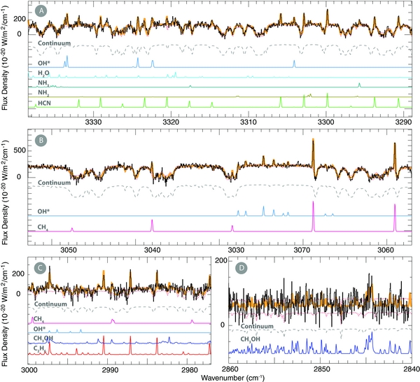
Figure 2. Detections of continuum and minor volatile species in C/2013 R1 (Lovejoy), along with H2O (or OH*, its direct proxy), extracted as in Figure 1. (A) HCN, NH2, OH*, H2O, and NH3 on November 7. (B) CH4 and OH* on November 7. (C) CH4, C2H6, CH3OH, and OH* on October 22. (D) CH3OH on October 22.
Download figure:
Standard image High-resolution imageTable 1. Retrieved Molecular Parameters for Primary and Product Volatiles in Comet C/2013 R1 (Lovejoy)a
| Species | νb | Lines | Trot | Global Qc | Abundanced |
|---|---|---|---|---|---|
| (cm−1) | (K) | (1026 s−1) | (% Relative to H2O) | ||
| 2013 October 22 | |||||
| eRh = 1.35 AU; Δ = 0.84 AU; Δ-dot = −40 km s−1; P.A. = 2808; α = 463. Time on source, KL1: 24 minutes, KL2: 28 minutes | |||||
| H2O | 3428.04 | 18 | 49 |
185.4 ± 19.2 | 100 |
| CH4 | 3041.70 | 5 | 54 |
1.54 ± 0.14 | 0.68 ± 0.12 |
| C2H6 | 2983.46 | 8 | 55 |
1.38 ± 0.17 | 0.72 ± 0.09 |
| CH3OH | 2850.53 | 17 | 46 |
5.40 ± 0.49 | 2.75 ± 0.38 |
| HCN | 3312.15 | 6 | (50)f | 0.59 ± 0.12 | 0.32 ± 0.07 |
| NH3 | 3295.41 | 1 | (50)f | <3.44 | <1.86 |
| NH2 | 3301.86 | 2 | (50)f | <0.35 | <0.19 |
| C2H2 | 3295.96 | 6 | (50)f | <0.92 | <0.50 |
| H2CO | 2780.97 | 12 | (50)f | <0.49 | <0.26 |
| 2013 October 24 | |||||
| eRh = 1.34 AU; Δ = 0.79 AU; Δ-dot = −39 km s−1; P.A. = 2814; α = 475. Time on source, M-wide: 14 minutes | |||||
| H2O | 2073.75 | 4 | (50)f | 153.2 ± 25.2 | 100 |
| CO | 2143.12 | 6 | 47 ± 3 | 15.15 ± 1.85 | 9.89 ± 2.03 |
| 2013 October 25 | |||||
| eRh = 1.33 AU; Δ = 0.77 AU; Δ-dot = −39 km s−1; P.A. = 2817; α = 481. Time on source, KL2: 28 minutes | |||||
| H2O | 3442.05 | 12 | 55 ± 10 | 231.8 ± 33.1 | 100 |
| CH4 | 3041.66 | 3 | 63 |
2.87 ± 0.17 | 1.24 ± 0.19 |
| C2H6 | 2904.94 | 9 | (50)f | 2.17 ± 0.35 | 0.94 ± 0.20 |
| HCN | 3313.65 | 10 | 54 |
0.68 ± 0.06 | 0.29 ± 0.05 |
| NH3 | 3315.17 | 2 | (50)f | <2.54 | <1.09 |
| NH2 | 3301.86 | 2 | (50)f | <0.22 | <0.10 |
| C2H2 | 3299.44 | 6 | (50)f | <0.15 | <0.07 |
| H2CO | 2779.99 | 12 | (50)f | <0.34 | <0.15 |
| 2013 October 27 | |||||
| eRh = 1.30 AU; Δ = 0.72 AU; Δ-dot = −38 km s−1; P.A. = 2822; α = 493. Time on source, KL2: 20 minutes | |||||
| H2O | 3446.17 | 9 | 62 ± 15 | 155.6 ± 24.9 | 100 |
| CH4 | 3041.66 | 3 | 63 |
1.81 ± 0.25 | 1.16 ± 0.25 |
| C2H6 | 2908.57 | 4 | (60)f | 1.74 ± 0.37 | 1.12 ± 0.30 |
| HCN | 3305.63 | 9 | (60)f | 0.36 ± 0.10 | 0.23 ± 0.07 |
| NH3 | 3306.30 | 2 | (60)f | <0.36 | <0.23 |
| NH2 | 3304.94 | 3 | (60)f | <0.29 | <0.19 |
| C2H2 | 3296.59 | 7 | (60)f | <0.22 | <0.14 |
| H2CO | 2777.33 | 15 | (60)f | <0.30 | <0.19 |
| 2013 October 29 | |||||
| eRh = 1.28 AU; Δ = 0.68 AU; Δ-dot = −37 km s−1; P.A. = 2826; α = 506. Time on source, KL2: 24 minutes | |||||
| H2O | 3440.70 | 13 | 59 |
145.0 ± 40.9 | 100 |
| CH4 | 3048.09 | 5 | 63 |
1.81 ± 0.21 | 1.25 ± 0.38 |
| C2H6 | 2908.10 | 7 | (60)f | 1.08 ± 0.25 | 0.75 ± 0.27 |
| HCN | 3307.94 | 10 | 56 ± 5 | 0.47 ± 0.06 | 0.32 ± 0.10 |
| NH3 | 3306.25 | 2 | (60)f | <0.36 | <0.25 |
| NH2 | 3302.60 | 4 | (60)f | <0.33 | <0.22 |
| C2H2 | 3298.44 | 4 | (60)f | <0.17 | <0.12 |
| H2CO | 2779.17 | 13 | (60)f | <0.28 | <0.19 |
| 2013 November 7 | |||||
| eRh = 1.16 AU; Δ = 0.51 AU; Δ-dot = −29 km s−1; P.A. = 2852; α = 581. Time on source, KL2: 20 minutes | |||||
| H2O | 3450.15 | 9 | 70 ± 2 | 367.9 ± 25.8 | 100 |
| CH4 | 3048.09 | 5 | 61 ± 4 | 3.35 ± 0.25 | 0.91 ± 0.09 |
| C2H6 | 2907.58 | 10 | 72 |
2.18 ± 0.25 | 0.59 ± 0.08 |
| HCN | 3312.74 | 12 | 70 |
0.87 ± 0.07 | 0.24 ± 0.03 |
| NH3 | 3295.36 | 1 | (70)f | 0.36 ± 0.05 | 0.10 ± 0.02 |
| NH2 | 3304.99 | 3 | (70)f | 0.44 ± 0.26 | 0.12 ± 0.07 |
| C2H2 | 3305.13 | 6 | (70)f | <0.16 | <0.12 |
| H2CO | 2779.77 | 8 | (70)f | <0.23 | <0.06 |
Notes. aUncertainties represent 1σ, and upper limits represent 3σ. The reported error in production rate includes the line-by-line scatter in measured column densities, along with photon noise, systematic uncertainty in the removal of the cometary continuum, and (minor) uncertainty in rotational temperature. bMean wavenumber of all emission lines (used for this reduction) from a particular species. cGlobal production rate, after applying a measured growth factor to compensate slit losses. dWe also estimated the weighted mean relative abundance (%) for each species: CO (9.89 ± 2.03), CH3OH (2.75 ± 0.38), CH4 (0.91± 0.06), C2H6 (0.69 ± 0.06), HCN (0.26 ± 0.02), NH3 (0.10 ± 0.02), NH2 (0.12 ± 0.07), C2H2 (<0.07), and H2CO (<0.06). eRh: heliocentric distance; Δ: geocentric distance; Δ-dot: geocentric velocity; P.A.: position angle of the extended Sun–comet vector; α: solar phase (Sun–comet–Earth) angle. These values represent the mid-point of data acquisition. KL1, KL2, M-wide refer to standard NIRSPEC settings. fAssumed value based on retrieval of contemporary species.
Download table as: ASCIITypeset image
3.1. Rotational Temperatures
Near-IR spectroscopy is sensitive to molecular ro-vibrational transitions, and the ability to detect multiple emission lines grants an accurate determination of the molecular abundances in the coma. Sampling of each trace gas simultaneously with water (the most abundant ice in cometary nuclei) reveals its relative abundance ratio directly, and removes most sources of systematic error that are often introduced when measured separately. To accurately determine the production rate for each molecular species we need to establish its rotational temperature (Trot) with high precision. This is essential for characterizing correct rotational level populations. Once Trot is known, accurate production rates are determined using fluorescence models we developed for each species: H2O (Villanueva et al. 2012a), OH* (Bonev et al. 2006), C2H6 (Villanueva et al. 2011b; Radeva et al. 2011), CO, C2H2, and CH4 (Paganini et al. 2013; Villanueva et al. 2011a; Gibb et al. 2003), NH3, HCN (Villanueva et al. 2013; Lippi et al. 2013), NH2 (Kawakita & Mumma 2011), H2CO (DiSanti et al. 2006), and CH3OH (Villanueva et al. 2012b; DiSanti et al. 2013).
From the observed molecular emission lines, we retrieved rotational temperatures (Trot) for six molecules (H2O, CO, CH4, HCN, C2H6, and CH3OH). For species whose Trot could not be determined, e.g., due to insufficient lines, restricted energy range, and/or poor signal-to-noise ratio, we adopted a value based on the results of other simultaneously observed molecules in the coma. In support of this approach, all derived rotational temperatures were consistent (within the 1σ–2σ level) on each date, suggesting a common temperature among species in the inner coma, as we generally find for a given comet. Figure 3(A) shows a gradual (and expected) increase of rotational temperature (from ∼50 K to ∼70 K) with decreasing Rh. The best-fit temperature variation followed a power law in Rh of −2.0 (Trot = T1AU Rh−2.0 ± 0.2, with T1AU = (93 ± 3) K representing the fitted value extrapolated to Rh = 1 AU; see Figure 3). Although our measurements sample a relatively small range of Rh, this power law is consistent with "typical" values for other comets (e.g., see Biver et al. 1997, 1999).
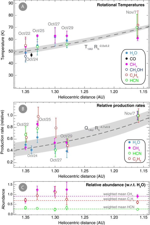
Figure 3. Temporal evolution of several key parameters in C/2013 R1 (Lovejoy), as revealed in our data. (A) Rotational temperatures retrieved for six gaseous species and their fitted trend line with heliocentric distance. (B) Individual production rates, scaled to the value obtained for each species on November 7, and their fitted trend line. (C) Abundances for CH4, C2H6, and HCN (%, relative to water) vs. heliocentric distance. The mean relative abundances were HCN/H2O = 0.26%, C2H6/H2O = 0.69%, and CH4/H2O = 0.9%. Some values are displaced horizontally for improved visibility, see Sections 3.1–3.3.
Download figure:
Standard image High-resolution image3.2. Production Rates
We performed observations of H2O, CH4, C2H6, and HCN simultaneously on five nights spanning October 22–29, and also on November 7. The water production rate increased from 1.0 × 1028 to 3.9 × 1028 molecules s−1 during this interval. On each night the measurements were nearly continuous over a span of 1 hr. We used these data to assess the evolution of abundances with Rh for these species.
Our best-fit results indicate a rather steep increase in water production with decreasing heliocentric distance (QH2O = Q1AU Rh−4.7 ± 0.9, with Q1AU = (6.66 ± 1.55) × 1028 s−1; Figure 3(B)), which is somewhat steeper than the typical (insolation-limited) value (Rh−2) often seen in comets (Biver et al. 1999). A steeper power law could be related to an increase in outgassing associated with (slow) nucleus rotation during this brief interval. Alternatively, the slope is strongly influenced by the data obtained on November 7 that could reflect a secular jump such as an outburst would trigger (cf. CBET 3710). Further inspection reveals a significant increase in production rates on October 25 compared to neighboring dates (see Figure 3(B)). Although the four volatiles (H2O, CH4, C2H6, and HCN) displayed clear absolute increases in production rate, only C2H6 and CH4 showed (at most, slight) enhancements in their abundances (relative to water), and only on October 25 and 27, while that of HCN remained fairly constant (i.e., data agree within 1σ; see Figure 3(C)).
With their lower sublimation temperatures, the increased abundance ratios for C2H6 and CH4 could perhaps be associated with a possible outburst triggered by another hypervolatile (e.g., CO or CO2). On previous dates we found CO to be enriched, suggesting that its production rate could vary on short timescales if it was mixed non-uniformly in the nucleus. However, the lack of simultaneous observations of CO (with C2H6 and CH4) precludes any conclusions on this possibility, and also on the distribution of CO in the nucleus. Nucleus rotation and associated variations in insolation of distinct active regions could introduce such variations, if such regions are compositionally distinct.
Finally, we obtained an ortho–para ratio (OPR) for H2O on October 22 using two instrument settings that spanned 3370–3520 cm−1. The intensities of 15 ortho–H2O and 6 para-H2O lines yielded an OPR of 3.01 ± 0.49, restricting the spin temperature to Tspin ⩾ 29 K (at the 1σ level).
3.3. Relative Abundances
Our observations of comet C/2013 R1 yielded absolute production rates for nine primary volatiles. Since water is observed simultaneously with each trace species, we obtained highly robust abundance ratios for seven trace volatiles (and upper limits for two additional species). The individual abundance ratios (with respect to H2O) for HCN, C2H6, and CH4 remained largely in agreement (within 1σ; Figure 3(C)) with their weighted mean values, despite the observed pronounced increase in gas production rates with decreasing Rh (Figure 3(B)). This suggests constant bulk volatile composition, regardless of variations in local activity (whether or not associated with nucleus rotation) during our observing campaign.
3.4. Spatial Profiles
We centered the slit on the comet and aligned it along the Sun–comet direction (Figure 4). From October 22 to November 7, the phase angle (i.e., the observer–comet–Sun angle) ranged between 46° and 58°. A viewing geometry with phase angle of 90° and the slit oriented along the Sun–comet direction would be "optimal," since all pixels at positive distances along the slit from the comet's center would sample the sunward hemisphere and all negative distances the anti-sunward hemisphere. Keeping this difference in mind, we will refer to the positive distances in Figure 4 as the projected "sunward" position, and negative distances as "anti-sunward" position.

Figure 4. Spatial profiles of primary volatiles and the continuum in comet C/2013 R1 on five nights. The directions of the Sun–comet vector and solar phase angle (both are projected onto the sky plane) are indicated relative to the slit orientation, which is horizontal for these plots. The observed spatial profiles for these emissions showed complex structures, possibly tied to nucleus rotation, or multiple jets (cf. CBET 3710). Profiles are discussed in Section 3.4.
Download figure:
Standard image High-resolution imageWe obtained spatial profiles for the continuum and for six parent volatiles (H2O, CO, CH4, HCN, C2H6, and CH3OH)—some of them on multiple dates. On October 22, ethane displayed sunward enhancements (to projected nucleocentric distance ∼2000 km), while H2O, HCN, and CH3OH showed symmetric profiles about the nucleus (extensions of CH3OH were measured only to ∼± 1000 km). The continuum, on the other hand, was enhanced in the anti-sunward direction. On October 24, our observations revealed asymmetric profiles for CO and the continuum, both enhanced toward the sunward side. On October 25 (when we observed an apparent increase in production rates), the spatial profiles of HCN and H2O were rather symmetric, while methane and the continuum favored release toward the sunward side. The behavior of methane showed similar enhancement (i.e., sunward release) on October 29 (as did HCN), while H2O showed flux excess in the anti-sunward direction (as did the continuum). On November 7, H2O, HCN, and CH4 showed slight enhancements in the sunward hemisphere, while the continuum was symmetric.
In summary, the complexity in our observed spatial profiles does not show clear delineation of outgassing sources as, for instance, would arise from polar and apolar ice phases—as was observed in comets C/2007 W1 (Boattini), 103P/Hartley2, and C/2009 P1 (Garradd; Villanueva et al. 2011a; Mumma et al. 2011; Paganini et al. 2012b). The evolving patterns in the profiles measured for C/2013 R1, however, could be related to nucleus rotation or to alternative physical effects like sequential activation of multiple outgassing jets (cf. CBET 3710). Additional observations at other wavelengths could test this possibility.
4. DISCUSSION: THE CO-RICH COMETS
Thanks to a combination of prompt observing strategies, technical advances, and a rigorous survey, we have quantified CO, H2O, and other volatile species in 17 OC comets since 1996, of which four were rich in native CO. Indeed, in comet C/2013 R1, the measured CO abundance (∼10%, relative to H2O) was enhanced, classifying it as a CO-rich comet—the fifth highest among the 17 comets from the ground-based IR survey.
But how common are these CO-rich comets? Are they outliers of the typical population of comets? Three other surveys (all space-based) sampled CO and H2O simultaneously (or nearly so) with the same beam size: the Akari IR survey (H2O is sampled directly) and UV surveys with Hubble and the International Ultraviolet Explorer (using OH as the proxy for H2O).
Among comets surveyed in the water-activated zone (Rh < 2.5 AU), Akari found that 6 of 13 comets were CO-poor (3σ upper limits less than 4.3% with respect to H2O), contrasting strongly with the fact that 11 of 13 showed significant CO2 abundance (>10% with respect to H2O; Ootsubo et al. 2012). Of these 13 comets, only 3 were OC comets, and only C/2008 Q3 (at Rh = 1.8 AU) showed high abundance ratios for both CO and CO2, (∼24% and ∼30%, respectively). Considering the large Akari aperture for the C/2008 Q3 observations (diameter of ∼27,000 km), some fraction of the CO observed in it could have been produced by dissociation of precursors such as CO2, H2CO, or by polymers such as polyoxymethylene (Eberhardt 1999; Fray et al. 2006). In the entire survey (at all heliocentric distances), CO was detected in only 3 of 18 comets sampled: C/2008 Q3 (Garradd), C/2006 W3 (Christensen) at 3.13 and 3.61 AU, and 29P/Schwassmann–Wachmann 1 at 6.18 AU. The lack of CO detections in most comets by the Akari survey is intriguing, although the sensitivity for CO (∼2 × 1026 molecules s−1, 3σ detection limit) could have restricted further detections.
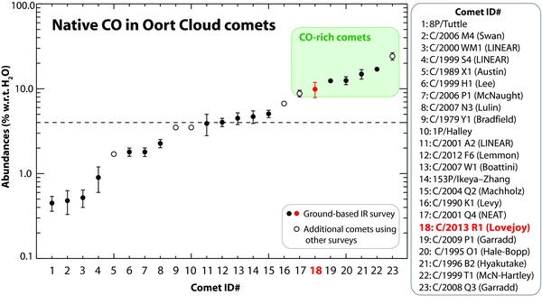
Figure 5 displays the CO/H2O mixing ratios based on the ground-based IR survey (17 OC comets; filled circles), with the addition of (6 OC) comets for which there were no ground-based IR results (open circles). We excluded ECs to avoid any biases, such as could be produced by (possible) CO depletion after multiple perihelion passages.
Figure 5. CO abundance ratios in Oort Cloud (OC) comets included in our IR survey. We also show results for (OC) comets C/1979 Y1, C/1989 X1, C/1990 K1, C/2001 Q4, and 1P/Halley from the UV surveys, and C/2008 Q3 from the Akari survey. For comets C/1990 K1 and C/2008 Q3, we used the weighted mean of measured CO abundances. The median abundance in this sample is ∼4% (CO, relative to H2O) and the range extends from ∼0.3% to ∼30%; see Section 4 for further details. References: 1: Böhnhardt et al. (2008); 2: DiSanti et al. (2009); 3: Radeva et al. (2010); 4: Mumma et al. (2001a); 5: Feldman et al. (1997); 6: Dello Russo et al. (2009); 7: Mumma et al. (2001b); 8: Gibb et al. (2012); 9: Feldman et al. (1997); 10: Eberhardt et al. (1999); 11: Magee-Sauer et al. (2008); 12: Paganini et al. (2014); 13: Villanueva et al. (2011a); 14: DiSanti et al. (2002); 15: Bonev et al. (2009); 16: Feldman et al. (1997); 17: Lupu et al. (2007); 18: This work; 19: Paganini et al. (2012b); 20: DiSanti et al. (1999, 2001); 21: Mumma et al. (1996), DiSanti et al. (2003); 22: Mumma et al. (2003); 23: Ootsubo et al. (2012).
Download figure:
Standard image High-resolution image
While the native CO abundances among comets show a range from ∼0.3% to values of about 30% (Figure 5), OC comets having high native CO abundances (>8%) seem to represent a small fraction of the sampled population. Considering a "typical" (median) abundance of ∼4% for CO (relative to H2O), we arbitrarily define comets with abundances larger than twice the median CO abundance (i.e., >8%) to represent "CO-rich" comets (shaded green in Figure 5). By this standard, the only comets rich in native CO are C/2001 Q4 (NEAT), C/1995 O1 (Hale-Bopp), C/1996 B2 (Hyakutake), C/1999 T1 (McNaught-Hartley), C/2009 P1 (Garradd; that also displayed larger CO values post-perihelion (e.g., Bodewits et al. 2014)), C/2008 Q3 (Garradd), and now C/2013 R1 (Lovejoy).
Could there be evidence of chemical post-processing in some comets? A'Hearn et al. (2012) showed that the relative depletion of CO (in ECs and NICs) was not proportional to the reciprocal of the semi-major axis (1/a). But they found that CO2 was somewhat depleted in comets with q < 1 AU, demonstrating the possible influence of thermal modification—but other hypervolatiles (like CO, CH4, C2H6) should then be depleted, too. The importance of CO is its high volatility (i.e., sensitivity to temperature), so high-CO comets have the potential to place important constraints on the birthplace and processing history of pre-cometary ices.
Can the relatively large CO content challenge and inform our current understanding of their origins? Recent mapping of the solar-nebula analog TW Hydrae with ALMA allowed estimates of the CO frost line (near ∼30 AU; Qi et al. 2013). Certainly, if we consider that the formation of comets occurred in the nebular mid-plane, a large CO abundance in these comets would support formation in cold regions near—or perhaps beyond—heliocentric distances that are consistent with the CO snowline. Earlier consideration of the severely depleted comet C/1999 S4 (and others) suggested formation in the Jupiter–Saturn zone where CO ice is not stable (Mumma et al. 2001a). However, the possible roles of radial mixing, shielding of certain hypervolatiles in water ice mantles, and the existence of diverse structural phases of ice, i.e., polar (H2O-rich) and apolar (CO-rich, CO2-rich), could serve as plausible explanations for the wide dispersion of CO content found in comets (e.g., Paganini et al. 2012b, for a discussion). We can only expect to sharpen our conclusions and answer these questions as future observations of CO-rich comets become available and dynamical models deal with the wide range of CO abundances in comets.
5. SUMMARY
Our NIRSPEC observations of comet C/2013 R1 resulted in detections of seven primary volatiles (H2O, CO, CH4, HCN, C2H6, CH3OH, and NH3), upper limits for two others (C2H2 and H2CO), and detections of two product species (OH* and NH2) at pre-perihelion distances (1.35–1.16 AU) in 2013 October/November. During this period, the measured production rate for water increased from 1.0 to 3.9 × 1028 molecules s−1. We measured (weighted) mean abundances (%, relative to water) for CO (9.89 ± 2.03), CH3OH (2.75 ± 0.38), CH4 (0.91 ± 0.06), C2H6 (0.69 ± 0.06), HCN (0.26 ± 0.02), NH3 (0.10 ± 0.02), NH2 (0.12 ± 0.07), C2H2 (<0.07), and H2CO (<0.06). We obtained consistent rotational temperatures (at the 1σ–2σ level) for six species (H2O, CO, CH4, HCN, C2H6, and CH3OH), suggesting a common source of rotational excitation within NIRSPEC's FOV on each date. The OPR for H2O was 3.01 ± 0.49, corresponding to a spin temperature larger than 29 K (at the 1σ level). Our results demonstrate a rich chemistry that, compared to most OC comets, reveals highly enriched CO, (at most) slightly enriched CH3OH, C2H6, and HCN, and CH4 consistent with "normal," yet depleted NH3, C2H2, and H2CO. NH2 was also depleted, as expected if it is the principal product of NH3 photolysis.
We have identified a new CO-rich comet. Future observations will test whether these comets stem from a larger population and, if so, assess whether the observed large CO abundance could indeed inform our understanding of the true formative conditions experienced by these icy bodies.
We gratefully acknowledge support by NASA's PAST Program (L.P., M.J.M, M.A.D., G.L.V.) and NAI through its member Teams at GSFC (M.J.M., M.A.D., B.P.B., G.A.B.) and at UH (J.V.K., K.J.M.; No. NNA09DA77A), and NSF (B.P.B., E.L.G.; Award 1211362). The data of October 24 and 25 were collected during part of the NASA Keck time awarded for observations of comet ISON, and are publicly available through the Keck Observatory Archive. We thank the anonymous referee for useful insights on this paper. The authors acknowledge the very significant cultural role and reverence that the summit of Mauna Kea has always had within the indigenous Hawaiian community. We are most fortunate to have the opportunity to conduct observations from this mountain.