


ABSTRACT
The internal pattern and overall magnitude of tidal heating for spin-synchronous terrestrial exoplanets from 1 to 2.5 RE is investigated using a propagator matrix method for a variety of layer structures. Particular attention is paid to ice–silicate hybrid super-Earths, where a significant ice mantle is modeled to rest atop an iron-silicate core, and may or may not contain a liquid water ocean. We find multilayer modeling often increases tidal dissipation relative to a homogeneous model, across multiple orbital periods, due to the ability to include smaller volume low viscosity regions, and the added flexure allowed by liquid layers. Gradations in parameters with depth are explored, such as allowed by the Preliminary Earth Reference Model. For ice–silicate hybrid worlds, dramatically greater dissipation is possible beyond the case of a silicate mantle only, allowing non-negligible tidal activity to extend to greater orbital periods than previously predicted. Surface patterns of tidal heating are found to potentially be useful for distinguishing internal structure. The influence of ice mantle depth and water ocean size and position are shown for a range of forcing frequencies. Rates of orbital circularization are found to be 10–100 times faster than standard predictions for Earth-analog planets when interiors are moderately warmer than the modern Earth, as well as for a diverse range of ice–silicate hybrid super-Earths. Circularization rates are shown to be significantly longer for planets with layers equivalent to an ocean-free modern Earth, as well as for planets with high fractions of either ice or silicate melting.
Export citation and abstract BibTeX RIS
1. INTRODUCTION
One of the unexpected discoveries that has come out of the rapid and ongoing growth in the number of known exoplanets is the wide distribution of orbital eccentricities in contrast to our own solar system. A similarly unexpected result has been the number of planets in short orbital periods, such as the population of Hot Jupiters and Hot Neptunes. Because two of the primary ingredients required to drive strong long-term tidal heating in a planetary body are high eccentricity, and proximity to a massive host, these two features of the exoplanet population taken together suggest a rich environment for planets within which tidal heating can play a significant role. Even if the orbital conditions to maintain steady long-term tidal heating, such as the mean motion resonance configuration of the Galilean moon system of Jupiter, remain rare in exosystems, we still desire improvements in our understanding of the tidal response of terrestrial worlds in order to better model their orbital evolution and damping, and to help inform the selection of Quality factors (Q) used for astronomical studies of terrestrial class objects.
There are three core reasons why it is critical to study the allowable rates of tidal heating in terrestrial class exoplanets at this time. First, there is simply the desire to understand specific planets in terms of their internal heating, temperature histories, and levels of volcanism. Second, tidal heating plays a central role in the stability of planetary orbits. Planets with high tidal dissipation may circularize rapidly from high eccentricities, reducing the probability of orbit crossings with other nearby objects, and thus reducing the probability of close encounters and scattering events (e.g., Chatterjee et al. 2008; Matsumura et al. 2013, 2010b). Low tidal dissipation, primarily caused by the melting of initially solid material, may allow high eccentricities to remain for far longer timescales, and reduce overall terrestrial planet stability. Lastly, emerging theories for the formation of short period extrasolar planets are based on tidal circularization from high eccentricity scattered orbits, and the limits of tidal heating in terrestrial class exoplanets is central to determining if such a mechanism is applicable to this category of worlds.
Eccentricities in the overall extrasolar planet population are proving to be far higher than initially expected (Tremaine & Zakamska 2004; Namouni 2005; Butler et al. 2006; Udry & Santos 2007; Matsumura et al. 2008; Schneider 2014). High eccentricities are found not only for long period or high-mass Jupiter class targets, but also for many short-period objects, including members of the growing catalog of super-Earths (objects with roughly 1 to 10 Earth-masses (ME)). While eccentricities show a gradual trend toward more circular orbits at short periods, with some planets at zero eccentricity, there remains a significant population across all mass classes at higher eccentricities even for very close-in orbits. Eccentricity values are difficult to measure for exoplanets, and are often reported based on the best fit of radial velocity lightcurves to multiple orbital elements. In some cases values may be overestimated (Shen & Turner 2008; Zakamska et al. 2011; Pont et al. 2011), while in other cases short period planets are only assumed to have zero eccentricity based on presumed rapid tidal circularization timescales in order to refine the fit of other parameters. In a few cases eccentricity is cautiously not reported. Despite such uncertainties, the broad distribution of eccentricities remains in need of explanation. Theories for the cause of high eccentricities include: ongoing circularization (e.g., Matsumura et al. 2008), the prevalence of early scattering, unseen outer perturbers, and the Kozai mechanism (Kozai 1962; Lidov 1962) where high inclination perturbers interact with inner objects.
Early theories for the formation of Hot Jupiters and Hot Neptunes focused upon the role of migration induced by early disk interactions. More recently it has been proposed that planet-planet scattering in early solar systems followed by tidal circularization may better explain certain features of the observed short period population (Ford & Rasio 2006; Fabrycky & Tremaine 2007; Wu et al. 2007; Nagasawa et al. 2008; Wu & Lithwick 2011). The discovery of a sub-population of Hot Jupiters with their orbits misaligned to the spin axis of their host stars, as determined by the Rossiter–McLaughlin effect, is difficult to explain by alternative migration theories (Ohta et al. 2005; Triaud et al. 2010; Winn et al. 2010). For gas giant planets, the high tidal dissipation rates required for circularization down from high eccentricities needed to explain this population has led to research on enhanced tidal dissipation in gas giant interiors.
Numerous super-Earths also exist in short period orbits, although population statistics are not fully clear on if their presence in such positions is high or low compared to other orbital regions. Howard et al. (2012) find that for solar-type stars, a super-Earth excess at very short periods analogous to the Hot Jupiters does not appear to exist in the Kepler catalog. The eccentricities meanwhile of most Earth and sub-Earth class exoplanets are not yet well established. The existence of short period terrestrial class worlds, however, is sufficient to motivate analysis of their past and present tidal behavior. Whether formed in-situ or via migration, the role of layer structures and of alteration via melting is essential for understanding the tidal dynamics of these worlds. In previous work (Henning et al. 2009), we analyzed the eccentricity component of tidal heating of terrestrial exoplanets using a variety of temperature-dependent viscoelastic homogenous interior models, looking at overall features of a possible tidally active population in terms of observability. This work indicated that for exoplanets with periods under ∼20–30 days around G to K class stars, extreme heating results are easily possible at modest eccentricities for Earth-sized worlds. Solutions with extreme heat production, on the order of thousands to millions of times the ∼44 terawatt (TW) heat rate of the modern Earth, are obtained using both the standard fixed Quality factor approach, as well as using viscoelastic methods including melting. This analysis, however, considered melting as a homogeneous phenomenon, with a single melt fraction to describe the entire planetary mantle. Real systems may instead experience strong stratification, and subsequently require an advanced method to determine true tidal outcomes and the resulting constraints on orbital evolution.
In this paper we update this approach by considering multilayered models. A multilayer method is necessary both as a prerequisite for models which track the production of partial melt in extreme worlds, and for the more basic purpose of improving the accuracy of tidal heat production predictions even in less extreme cases where material layers remain largely unmelted. Many authors have investigated the tidal response of the solid Earth (e.g., Wahr 1981; Dehant 1987; Mathews et al. 1995; Wang 1997), including the use of multiple layers, but generally with a focus upon Love numbers at the surface, and not on the distribution and magnitude of heating in extrasolar Earth-analog cases as explored here. Super-Earth planets (Valencia et al. 2006, 2007b) are of particular interest in this work, due to the natural selection bias of most exoplanet detection methods toward larger bodies. Regardless of the galactic population, there will be a large number of super-Earth worlds for which we will wish to have a robust understanding of the their tidal response behavior.
In previous work we have treated super-Earth worlds as scaled-up Earth analogs dominated by iron and silicate, however, studies (Raymond et al. 2004, 2006, 2009; Mandell et al. 2007; Valencia et al. 2007a; Fu et al. 2010) suggest that it will be common for super-Earths to have accreted large ice mantles. Indeed, it can be expected that there is a continuum of planetary compositions from super-Earths, into mini-Neptunes (Barnes et al. 2009; de Mooij et al. 2012), on up to the deep ice mantles of full Neptune-class worlds. For this reason, in this study we also examine the tidal impact of adding ice mantles to generate ice–silicate hybrid planets within the Earth to super-Earth mass range.
It is important to emphasize that tidal heating values reported in this work are for eccentricity-tides only, and are based on an assumption of spin-synchronization relative to the orbital host. This assumption is best at very short orbital periods, however, it is not guaranteed, and some short period exoplanets may instead lock to higher spin-orbit resonances other than 1:1. Makarov et al. (2012) and Makarov & Berghea (2014) have suggested such higher order spin states for GJ 581 d and GJ 667C c respectively, based on advanced rheology models. For the same reason that the timescales for spin-synchronization and obliquity damping are often assumed to be short (on the order of a few millions of years) in proximity to a massive host, heating from such tidal components is expected to be very large, and if present may readily contribute to global-scale melting. The total tidal heating with ongoing spin, obliquity, and eccentricity tides may be approximated by a linear sum of contributions (e.g., Wahr et al. 2009, Equation (1), or Jara-Orué & Vermeersen 2011, Equation (2)), although at similar periods summation at the tidal potential stage will not always translate into summation of net deformation, and the material result will be complex if for example one additional heat source shifts a layer across a threshold into a partial melt regime. If heating from any ongoing non-synchronous spin tides is moderate, then it may here be considered akin to the additional radionuclide heating of young planets, as both would bias a planet toward hot and high melt-fraction eccentricity-tide solutions. In addition, note that only values computed after application of the eccentric external tidal forcing potential (such as heat production rates; see the Appendix) embed an eccentricity-tide only assumption, while results prior to application of the tidal potential such as Love numbers, and the radial distribution of deformation, are functions of the assumed layer structure and forcing frequency only.
In Section 2 we discuss general issues for tidal modeling. In Section 3 we describe the propagator method for computing multilayer tides, along with selection criteria for material parameters. In Section 4 we report results for Earth analog worlds of 1 RE, and then for ice–silicate hybrid worlds up to 2.5 RE. In Section 5 we discuss the impact of water ocean presence, position, and size, as well as the impact of gradations in material properties and the production of magma oceans.
2. BACKGROUND
Fundamental tidal heating theory (Darwin 1879; Love 1927; Munk & MacDonald 1960; Kaula 1968; Zschau 1978; Platzman 1984) has been used to extensively study solar system targets, including silicate systems such as Earth's moon (Peale & Cassen 1978), and Io (e.g., Peale et al. 1979; Reynolds et al. 1980; Yoder & Peale 1981; Fischer & Spohn 1990; Tackley et al. 2001; Hussmann & Spohn 2004), and for ice–silicate hybrid systems such as Europa (e.g., Cassen et al. 1979; Squyres et al. 1983; Ojakangas & Stevenson 1989; Moore & Schubert 2000; Showman 2003; Moore 2003a; Tobie et al. 2005; Hurford et al. 2005), Ganymede (Showman & Malhotra 1997), Enceladus (e.g., Meyer & Wisdom 2007; Hurford et al. 2007a; Roberts & Nimmo 2008), and many additional objects. More recently, numerous studies have investigated the role and impact of tidal heating and tidal evolution for terrestrial exoplanets (Jackson et al. 2008a, 2008c; Barnes et al. 2008, 2013; Henning et al. 2009; Bĕhounková et al. 2010, 2011; Matsumura et al. 2010a; Heller et al. 2011; Efroimsky 2012; Bolmont et al. 2013; Heller & Barnes 2013; Heller & Armstrong 2014) with an emphasis on habitable worlds, as well as multilayer tidal heating in the cores of gas giant planets (Remus et al. 2012a, 2012b; Storch & Lai 2014). Recently, Auclair-Desrotour et al. (2014) have investigated the role of frequency-dependent tidal damping on the orbital evolution of solid and fluid exoplanets.
To date, a handful of extrasolar super-Earths are already candidates for geologically significant tidal heating, including GJ 876 d (Rivera et al. 2005; Valencia et al. 2007b; Bean & Seifahrt 2009; Correia et al. 2010; Rivera et al. 2010b), 55 Cancri e (McArthur et al. 2004; Dawson & Fabrycky 2010), GJ 1214 b (Charbonneau et al. 2009), HD 1461 b (Rivera et al. 2010a), and GJ 667C b (Bonfils 2009). Super-Earths already detected with reported eccentricities of zero may also have experienced extreme tidal conditions in their past, such as CoRoT-7 b, CoRoT-7 c, Kepler-10 b, and Kepler-11 b (Queloz et al. 2009; Léger et al. 2009; Batalha et al. 2011; Lissauer et al. 2011). For these worlds, due to very short orbital periods, even very small eccentricities (e.g., below 0.001) may still generate geophysically significant tidal heating.
Large radii, as determined by transit, suggest some Hot Jupiters with higher eccentricities may be tidally active (Laughlin et al. 2005; Gu et al. 2003), such as HD209458 b (Bodenheimer et al. 2001, 2003), HAT-P-1 b (Bakos et al. 2007), and many recent objects, e.g., WASP-4 b, WASP-6 b, WASP12 b, WASP15 b, and TrES-4 (Ibgui et al. 2010). The discovery of the Neptune-class GJ 436 b at e = 0.150 ± 0.012 (Deming et al. 2007) with a period of only 2.64 days suggests potentially strong tidal activity. Such anomalies often hint at unseen companions. The resonant multi-body system GJ 876 b, c, d, e (Marcy et al. 1998, 2001; Rivera et al. 2005, 2010b) and the five-planet system 55 Cancri b, c, d, e, f (Marcy et al. 2002; Fischer et al. 2008) with the likely eccentric tidal planet 55 Cancri e (McArthur et al. 2004; Dawson & Fabrycky 2010) each suggest the importance and high prevalence of multiple planet interactions. Mean motion resonances, critical for sustaining long duration eccentricity driven tidal activity, already appear common and stable among exoplanet systems (Marcy et al. 2001; Lee & Peale 2002; Lee 2004; Haghighipour et al. 2003; Lecoanet et al. 2009), likely due to systematic assembly during convergent migration (Yu & Tremaine 2001), perhaps analogously to the Galilean moon system (Canup & Ward 2002). Tidal activity may also occur due to ongoing circularization alone (Jackson et al. 2008b). High inclination outer perturbers may also be responsible for driving some of the observed eccentricity distribution via the Kozai mechanism (Kozai 1962; Takeda & Rasio 2005).
Observability of such tidal activity faces numerous challenges (Kaltenegger et al. 2010). The primary issue is that to obtain high tidal response rates, a planet generally needs to be in a very close orbit around a host star, and there its surface environment is overwhelmingly dominated by insolation. For bright main sequence hosts, a planet, even despite tidal activity, may have a magma ocean solely due to insolation heating, e.g., CoRoT-7 b (Barnes et al. 2010; Léger et al. 2011). Spin synchronization may restrict the highest insolation levels to one face of a planet, but even modest atmospheres may be sufficient to transport enough heat to a nightside to mask the few degrees Kelvin change typically possible from tidal enhancement.
For ice-hybrid worlds we focus here additionally on colder terrestrial planetary cases, where surface water ice is plausible, and tidal heat competes less with insolation for significance. This category will include exomoons (Barnes & O'Brien 2002; Scharf 2006; Heller & Barnes 2013), where it is easier for tidal heating to play a more dominant role due to arbitrary distances from a host star (Stevenson 1999; Debes & Sigurdsson 2007), but detectability may be further off. Kepler-class photometry (Borucki et al. 2008) may have sufficient sensitivity in low noise cases to begin detecting extrasolar moons (Kipping et al. 2009). Tidal heating scales roughly by the fifth power of body radius, and the second power of host mass (Equation (1)), and therefore larger icy exomoons, around nonluminous hosts at or above Jupiter's mass, will be particularly susceptible to tidal activity.
3. METHODS
The basis of computing tidal dissipation for layered self-gravitating planetary bodies is a method known as the propagator matrix technique (Love 1927; Alterman et al. 1959; Takeuchi et al. 1962; Peltier 1974; Sabadini & Vermeersen 2004). Details of this method are given in the Appendix, and are further presented in comprehensive detail in Sabadini & Vermeersen (2004). As input, this technique takes a model world composed of spherically symmetric shells, each with prescribed density, shear modulus, and viscosity. An external gravitational potential, typically a degree 2 tidal disturbance of a given magnitude, is then applied to this model body. Boundary conditions are solved at each interface to yield solutions for the radial and tangential displacements, strains, and stresses. The result of the propagator matrix approach is a set of coefficient functions which are then composed into full 9 × 9 element stress and strain tensors in spherical coordinates and combined to determine the work per unit volume.
The viscoelastic solution is found by computing the purely elastic solution for the system of propagator equations resulting from the above methods, then invoking the viscoelastic-elastic correspondence principle (Biot 1954; Peltier 1974; Henning et al. 2009). In the complex-valued viscoelastic solution (a Fourier domain approach), the imaginary component of the computed work carries the information for the energy lost per cycle, and thus the tidal dissipation rate, while the real component represents instantaneous stored elastic energy. This technique leads to maps of tidal dissipation in each layer in latitude and longitude, each averaged over one orbit, which may then be summed over depth. Dissipation integrated over all layers is often assumed to represent a useful first approximation of the equilibrium surface flux of heat, or in particular, the flux of heat prior to re-distribution into heat pipes, perhaps at the base of an object's lithosphere.
In addition, Tobie et al. (2005) report a fast method for multilayer tidal computation, which determines the distribution of heating with depth for a given layer structure, while not resolving the solution in latitude and longitude. This approach has been used here to double-check for numerical error buildup in other methods, as well as to perform high grid density studies in depth.
The propagator method traditionally handles boundary conditions for solid-solid interfaces, however, our code has been extended following Jara-Orué & Vermeersen (2011), to handle layer interfaces with static liquid layers which propagate neither displacement nor stress. We note this method uses an alternative to the more common Fourier domain approach for viscoelasticity, through the Laplace domain, however, for a harmonic periodic system, results such as surface Love numbers and total dissipation are the same as from the Fourier methods above. In addition, we have computed liquid layer results using the TideLab suite of code provided by William Moore (Moore & Schubert 2000), which generates the propagator solution for a planetary model using a separate method in which the core-to-surface propagation of gravitational (liquid and solid layers) and mechanical (solid layers only) terms are mathematically separated (Wolf 1994). These two methods were used as checks on one another for validation purposes.
In this work we have chosen to only implement the viscoelastic Maxwell rheology (e.g., Bland 1960; Nowick & Berry 1972; Spada 2009), but other rheologies may also be useful for extrasolar worlds. Alternatives include both the Burgers rheology, helpful for modeling multiple grain scale creep mechanisms (Burgers 1935; Zener 1941; Sabadini et al. 1987; Faul & Jackson 2005; Henning et al. 2009), and the Andrade model (e.g., Efroimsky & Williams 2009; Efroimsky 2012; Shoji et al. 2013), which can be tuned to achieve a material response closer to the weak frequency dependence often observed in laboratory creep response tests (Karato & Spetzler 1990; Gribb & Cooper 1998). In the Andrade model, a rheology is primarily characterized by an empirically determined power law coefficient, commonly designated α, however, a drawback of the technique is that this parameter is not directly linked to the material properties of viscosity and shear modulus. To help limit the already very large number of free parameters in this work, and because it allows characterization of planetary responses in terms of true viscoelastic material parameters, the Maxwell model was utilized here. The primary impact of both the Burgers and Andrade models is to broaden the material resonance peak in the frequency domain, reducing the effective frequency dependence of Q, and bringing the tidal response closer to that of the fifth power of mean motion dependence of a fixed Q approach in the region of a broadened peak. Conversely, the only major weakness of the Maxwell rheology is that its frequency dependence may be greater than real systems. Therefore, one may keep in mind how such advanced rheologies are likely to impact future work, by reducing the sensitivity of results in this work to tidal forcing frequency or orbital period.
In general, such planet modeling is limited by the very large number of unknown parameters. When gradations of parameters are considered, the number of degrees of freedom becomes potentially infinite. It is therefore our goal not to model all possible variability and material physics, but to constrain the top level behavior of multilayer rocky and icy planets, while identifying the smaller subset of degrees of freedom which are of primary importance. We also seek to determine which structural features matter most for the response, and why. Henning et al. (2009) includes detailed discussion of the impact of material melting on tidal exoplanets addressed only briefly here. Valencia et al. (2006) and Valencia et al. (2007a) include detailed discussion of the impact of various equations of state on structure.
3.1. Classical Tidal Equations
Results are compared with a homogeneous tidal heating approach for exoplanets, described in detail in Henning et al. (2009). The problem of computing the tidal heat production rate for a simplified planetary body is approached using the viscoelastic form of the standard homogeneous tidal equation (Segatz et al. 1988):

where each parameter is given in Table 1, and Im(k2) is the imaginary component of the complex valued load Love number. This term contains all information in this equation regarding viscous dissipation in the material, and is derived from a material's constitutive equation and complex valued rigidity. In Henning et al. (2009) Im(k2) was computed for the Maxwell, Standard Anelastic Solid, and Burgers rheologies.
Table 1. Symbols and Parameters
| Parameter | Symbol |
|---|---|
| Tidal heat rate | W |
| Semimajor axis | a |
| Eccentricity | e |
| Mass of the primary | Mpri |
| Mass of the secondary | Msec |
| Radius of the secondary | Rsec |
| Second-order gravitational Love number | k2 |
| Second-order radial displacement Love number | h2 |
| Second-order tangential displacement Love–Shida number | l2 |
| Orbital mean motion | n |
| Orbital period | P |
| Pressure | p |
| Temperature | T |
| Ice layer thickness | tice |
| Displacement | ur, uθ, uϕ |
| Strain |  |
| Stress | σ |
| Internal gravitational potential | φ |
| External gravitational potential | Φ |
| Gravitational potential stress | ψ |
| Colatitude | θ |
| Longitude | ϕ |
| Colatitude relative to tidal symmetry axis | θT |
| Longitude relative to tidal symmetry axis | ϕT |
| Harmonic degree | ℓ |
| Density | ρ |
| Propagator matrix | Y |
| Aggregate propagator matrix | B |
| Propagator boundary matrix | M |
| Propagator solution vector | y |
| Propagator solution kernel | c |
| Propagator boundary vector | b |
| Seismic parameter | β |
| Quality factor | Q |
| Circularization timescale | τcirc |
| Maxwell timescale | τMax |
| Universal gas constant | R |
| Gravitational constant | G |
| Defining viscosity | ηo |
| Viscosity setpoint | ηset |
| Shear modulus | μ |
| Activation energy | E* |
| Activation volume | V* |
Download table as: ASCIITypeset image
The classical tidal circularization timescale may be written in terms of the energy loss rate to tides (Goldreich & Soter 1966; Murray & Dermott 2005),

where the (1 − e2) term can be neglected at small e. This form of the equation assumes negligible eccentricity change due to the tidal bulge raised on the primary by the secondary, which is true for most cases of a terrestrial class planet and star. This form of the circularization equation, in terms of Wtidal instead of in terms of Q, highlights the fact that circularization rates depend on a quantity that is time-dependent, and will vary both with the evolution of the system frequency n, and the internal planetary temperature.
Other forms of this equation expand Wtidal as in Equation (1), allowing cancelation of terms; however, this neglects verifying if a given planet is capable of supporting a particular dissipation rate. If during circularization, large-scale melting occurs, then Wtidal will change. In many cases, melting will lead to piped advection of melt (O'Reilly & Davies 1981; Moore 2001; Monnereau & Dubuffet 2002; Connolly et al. 2009; Spiegelman 1993; Ribe 1987) either to a surface ocean, subsurface ocean, or both. Addition of an ocean to an otherwise initially solid world can have a significant impact of the total tidal dissipation, and thus alter τcirc, as discussed in Section 5.
3.2. Quality Factors
Quality factors, introduced from seismology, are a useful although occasionally misleading aggregate scalar factor to describe inverse energy loss per cycle of a damped oscillator. Q factors are often treated as effectively constant, although in reality they are strong functions of forcing frequency, temperature, layer structure, and numerous internal material properties that vary with time. Values of Q are related to the lag angle of a tidal bulge t via the formula: Q = sin |t|. For Earth, a Q of 12–34 has been measured based on the expansion of the moon's orbit (Yoder 1995; Dickey et al. 1994; Murray & Dermott 2005); however, such low values (thus high dissipation) are due to the lunar-tide induced flow in Earth's water ocean. Goldreich & Soter (1966) estimated Q for Mercury, Venus, and the Moon as Qmerc ⩽ 190, Qvenus ⩽ 17, and 10 ⩽ Qmoon ⩽ 150. However, these values for Venus and Mercury make several assumptions about each world's spin history. Lainey et al. (2007) recently estimated Qmars = 79.91 (±0.69) from the motion of Phobos. Data summarized in Karato & Spetzler (1990) suggest Earth's lower mantle Q at tidal periods from 1–10 days is in the range 50–200. Based on such results, a common assumption for a dry 1 ME exoplanet has been the round number 100. In reality, Q is coupled in a viscoelastic system with the second order tidal Love number k2 (Segatz et al. 1988), leading to the value Im(k2) in Equation (1), which replaces the ratio k2/Q in the non-viscoelastic form of Equation (1) (e.g., Peale et al. 1979). For use in common astrophysical equations, however, it is often useful to extract from Im(k2) an effective Q value, by the formula Qeff = Re(k2)/− Im(k2). Earth-sized effective Q values range as far as ∼1–107.
For solid bodies, the common practice of adopting a fixed Q factor and calculating a resulting circularization time can lead to completely incorrect predictions, because it skips the step of examining if the tidal heating rate of the planet is realistic or sustainable. Consider GJ 876 d, with a minimum mass of 6.8 ME, period of 1.937 days, and host mass of 0.33 Msol. Using a fixed Q of 100 for this world leads to a rapid circularization timescale of 4 million years. This, however, would require the planet output 80 million TW of power for all 4 million years, which is extremely unlikely (the global heat rate of the modern Earth is only ∼44 TW). Instead, the planet will experience global-scale partial melting, altering the initial assumed Q. Using a tidal equilibrium model (Section 3.3) with partial melting, and a starting eccentricity of 0.139 (Correia et al. 2010), leads to a valid sustainable tidal dissipation rate of only 80,000 TW, equivalent to a global effective Q value of 100,000, and a circularization timescale of 4 billion years. A main argument to proceed with the research in this work is the primary concern of fixed Q models for icy or rocky planets, namely that Q is highly sensitive to internal structure, and the need to assess how Q (or by proxy Im(k2)) varies when global-scale partial melting or liquid magma or water ocean layers exist. This work may be seen as a precursor to the larger goal of assessing the tidal evolution of systems including terrestrial planets in time, particularly during orbital scattering and circularization, when such ocean layers (or simply hotter and less viscous layers) are very likely to develop.
3.3. Material Models
Our goal is to understand the grand scale differences in the response of planets of different bulk structures, at a time when even the rheological details of Earth's own deep interior remain in debate. For bulk tidal dissipation as a function of depth, the critical parameters are the viscosity, shear modulus, and density, with viscosity by far exceeding all other parameters in terms of control of the final tidal outcome. This dominance of viscosity allows one to begin with several simplifying assumptions in regards to density, rigidity, and composition.
For a homogenous Maxwell rheology planet, −Im(k2) in Equation (1) may be expressed analytically (Henning et al. 2009)
where η is viscosity (in Pascal-seconds), μ is the shear modulus (sometimes referred to as rigidity), ω is the forcing frequency, ρ is the homogeneous planet density, g is surface gravity, and Rsec the planet radius. Similar expressions may be written for other rheologies (Henning et al. 2009). Note that Equation (3) embeds an assumption of incompressibility by considering only deviatoric stress components within a world, and can thus become less accurate for large worlds such as mini-Neptune class planets.
While it is possible to write the analytical expression of Im(k2) for multilayer planets, even for two-layer bodies such expressions rapidly become impractical to work with. For several layers, they readily require several pages to express. We therefore shift to staged numerical computation to determine Im(k2) in multilayer cases. The essential character of Equation (3), however, remains the same, in that outcomes are a result of η, μ, and ρ for each layer.
For the shear modulus of silicates we adopt a baseline value of 5 × 10¹⁰ Pa unless otherwise noted, such as in some Earth models below. For solid ice, we adopt a standard value of 4 × 10⁹ Pa. While other works use a variety of shear modulus values for both material classes, what is most important (especially considering the unknown role of impurities) is the comparatively very small range of uncertainty in this parameter relative to uncertainty in viscosity. In general, impurities weaken a pure crystalline material, and therefore the inclusion in water ice of other volatiles such as CO2, NH3, and CH4, either as clathrates or as ices themselves, may be considered in a simplified fashion by considering lowered μ values. Because of high pressures, weakening due to faults and material damage is not a major consideration below the first 1–2 km of a major planet.
Viscoelastic materials typically experience a material resonance as a function of forcing frequency (see e.g., Nowick & Berry 1972), at which maximum dissipation occurs. For the Maxwell rheology, this peak response occurs when a forcing period equals the Maxwell timescale τMax = η/μ. A multilayer planet will not have one characteristic Maxwell timescale but many, and different layers will resonate at different forcing rates. Typical Maxwell times for silicates are shown in Figure 1 and cover a broad range from hours to years. For typical ice with a viscosity of 1013, 1014, and 1015 Pa s, τMax = 0.6 hr, 6.9 hr, and 2.8 days. The relative separation between material layer Maxwell times and forcing periods plays a central role in determining tidal outcomes. Layers that are viscoelastically well-matched to their forcing periods generally experience the highest tidal heating rates. For silicates the very wide distribution of η and μ values makes estimation of behaviors difficult prior to more individualized analysis. For ices, most cooler material will have an optimal response in the lower typical range of planetary and exomoon periods.

Figure 1. Silicate material property variations. Upper left: viscosity for a range of input parameters, including a baseline model set to match 1 × 10²¹ Pa s at T = 1000 K, as well as set points one order of magnitude above (strong) and below (weak) this baseline. An alternative activation energy is shown to modestly steepen the slope of viscosity with temperature. For higher pressures, it is clear that the slope generally becomes steeper, however, set point selection is unclear, and is chosen in these cases to match 1 × 10²² Pa s at T = 1500 K, roughly corresponding with the data available for the Earth's mid-to-upper mantle. What is clear is that any single parameterization leads to considerable uncertainty when high pressures are considered. Note the elevation in melting points at high pressures. Corresponding Maxwell times for the single shear modulus profile shown indicate optimal tidal coupling for many silicate models in the partial melt range.
Download figure:
Standard image High-resolution imageFor silicates and ices, shear moduli are nearly constant with temperature up until very near the melting temperature, at which point various models of shear weakening begin to occur (Fischer & Spohn 1990; Berckhemer et al. 1982). For pure water ice with a single melting temperature, the shear modulus falls directly to zero upon melting. Silicates melt across a range of temperatures, beginning at the solidus Tsol, with zero melt fraction, and ending at the liquidus Tliq with a melt fraction of 1.0 (with melt fraction varying linearly in temperature in between). A typical surface range for silicate melting is Tsol = 1600 K, and Tliq = 2000 K (Henning et al. 2009). Higher pressure melting points may be found via the Simon equation (Poirier 2000). The shear modulus for silicates remains close to its solid value for approximately half the melting range, and falls rapidly to zero at the point where individual mineral grains loose physical contact with one another, within a surrounding liquid bath. This point is referred to as the breakdown (or disaggregation) temperature Tbr, and typically lies between 40% and 60% melt fraction (Moore 2003b).
Density may be treated either by utilizing fixed average bulk values appropriate for a given layer, or through detailed equation of state calculations, which in turn depend on a temperature profile. Density primarily influences the elastic component of the load Love number (e.g., Re(k2)) for a planet on which tidal heating depends only linearly. Such Love numbers for the objects studied here vary typically by less than a factor of ∼2 due to the large overall mass. By contrast, viscosity variations may readily alter heat outputs by 4–5 orders of magnitude. Therefore, for simplicity we focus on cases with layer densities assigned (or in the case of Earth, taken from measurements) rather than calculated from equations of state and accompanying temperature/convection assumptions.
The tidal response of a planetary iron core is often weak, however, it is straightforward to include the core in multilayer calculations for completeness, and to verify such weakness, especially since it comes at little computational cost. Data on the viscosity of core analog Fe or Fe Ni alloy materials is limited. Frost & Ashby (1982) use a value of 1 × 10¹³ Pa s. Dumberry & Bloxham (2002) use a range from 1 × 10¹¹ to 1 × 10²⁰ Pa s. Buffett (1997) suggests a value less than 1 × 10¹⁶ Pa s. We discuss the results of such uncertainty further in Section 5.
Liquid metal in an outer core has very low viscosity. Ab initio methods by de Wijs et al. (1998) suggest values of 1.3 × 10⁻² Pa s for an inner core boundary at 6000 K, 1.2 × 10⁻² Pa s for a core mantle boundary of 4300 K, and 1.5 × 10⁻² Pa s for a core mantle boundary of 3500 K. Earth observations from the Chandler wobble and free oscillations however lead to high values of 104–1011 Pa s (Verhoogen 1974; Won & Kuo 1973) for the outer core. However, since even the highest value in this range is two orders of magnitude below the lowest solid viscosity used, tidal heating in any outer core is always found to be entirely negligible.
Viscosity is strongly dependent upon numerous material parameters, the most important of which is temperature. Pressure, grain size, and the total stress magnitude also play central roles. Stress state is most important for determining which modes of viscous behavior dominate the strain rate for an applied loading. Microscale viscous behavior may occur via diffusion creep (where crystal lattice voids migrate within grains), dislocation creep (the migration of linear lattice nonconformities known as dislocations), slippage along grain boundaries, or the diffusion of grain boundaries. Of these mechanisms, Moore (2006) demonstrates how diffusion creep dominates for ice under a wide range of tidal conditions and grain sizes.
As with shear moduli, in this work we focus on selecting informed estimates for viscosity in each material layer, as opposed to deriving such viscosities directly from a temperature and pressure profile. There are several reasons for this choice. First, the method of deriving viscosities from first principles at depth in a planetary body has not yet been fully successful even for the Earth, where postglacial rebound studies have provided measurements of the full mantle viscosity profile (Mitrovica & Forte 2004), but matching such values requires numerous posteriori adjustments to theoretical models, such as invoking the lateral inhomogeneity of rising and falling convection plumes and uncertainties in petrological composition. In reality, is it likely that the pressure dependence of planetary materials as currently modeled for low pressures does not extrapolate well to deep mantle pressures. For the Earth, rising temperatures act to lower viscosities, while high pressures act to raise viscosities, and results are extremely sensitive to which of these two processes is allowed to dominate, in effect meaning results are largely controlled by the choice of the activation volume V* (see Equation (4)), a value for which there is little laboratory data at high pressures.
In addition, deriving viscosities from a temperature and pressure model by depth inherently converts the problem into a highly unstable iterative computation. Two strong feedbacks are intertwined in this case. The vigor of convection, which determines upper boundary layer thicknesses and heat flux rates, is itself a strong function of viscosity. Second, heat flux rates depend upon the level of tidal heating, and thus tides strongly control planetary temperatures and viscosities. In reality, these feedbacks are resolved in time for a given orbit by an equilibrium between tidal heat input and convective heat loss. Planets will often evolve in time (typically a few million years) toward a very stable equilibrium temperature (Moore 2003b) where tidal heat input balances convective heat loss. In a large fraction of rheological and orbital cases (Henning et al. 2009), terrestrial exoplanets will reach tidal-convective equilibrium very close to either the solidus Tsol or breakdown Tbr temperatures. Therefore, for high tidal-heat Hot Earth cases, the most important viscosities to consider are those expected to reside near these states.
Previous analysis has mainly considered such tidal-convective equilibration for mantles characterized by a single bulk temperature and single melt fraction. While this is not a bad assumption for a well-mixed adiabatic convecting mantle, it may become significantly inappropriate once large-scale melting and melt mobilization begins for hotter planets. Multilayer models, where liquid or weak solid partial melt layers may be explicitly introduced along with homogeneous convecting layers, offer a significant improvement in their ability to determine a true range of tidal outcomes.
For silicates, viscosity prior to melting may be computed from an Arrhenius model

where R is the universal gas constant, E* is an activation energy, T is temperature, p is pressure, and V* is an activation volume. A defining viscosity ηo coefficient is calculated based on a viscous setpoint, for example, η(T = 1000 K) = ηset. In Figure 1 we use ηset = 1 × 10²⁰, 1 × 10²¹, 1 × 10²² Pa s for a weak, moderate, and strong silicate rheology, and compute a corresponding ηo for each. The low value for defining viscosity represents a more volatile-rich mantle (Hirth & Kohlstedt 1996), while the high value represents a more devolatilized case. Viscosity reductions due to temperature and melting occur on top of this setpoint selection. Therefore, ηset is a compositional choice, and is not the actual viscosity of a planet's mantle, which is likely to be much lower, due to a significant partial melt fraction.
A complex falloff of viscosity occurs for silicates near the solidus temperature (Moore 2001, 2003b; Fischer & Spohn 1990; Berckhemer et al. 1982). We omit the details of such models here, except to note that the minimum viscosity for silicate materials prior to complete melting is in the range 1 × 10¹²–1 × 10¹⁶ (a range notably similar to the viscosity of ice).
The majority of tidal dissipation on ice–silicate hybrid planets occurs within ice layers. For ice, viscosity prior to melting may be computed following Goldsby & Kohlstedt (2001),

where  is strain rate, Ax is a creep mechanism scale parameter, σ is stress, and h grain size. For volume diffusion creep, the exponent values are set at nσ = 1 and mg = 2, and we may follow Moore (2006) for Ice Ih to adopt Ax = 9.06 × 10⁻⁸/T Pa
 m
m s−1, E* = 59,400 J mol−1, and V* = −1.3 × 10⁻⁵ m3 mol−1. Typical values for h include the range 0.0001 to 0.01 m. Note that the activation volume here is negative, and therefore Ice Ih is expected to decrease in viscosity at higher pressures, unlike silicates that rise in viscosity. Figure 2 shows the results of Equation (5) for a range of pressures and temperatures appropriate for an exoplanet ice mantle. Typical pressures for such ice mantles are demonstrated in Figure 3. The pressure variation must be considered cautiously however, because the activation volume for high pressure ice phases, especially Ice X, are not well known. Figure 2 does, however, allow us our goal of a range of informed estimates for ice viscosities for the cases of interest, even if not dynamically linked by all feedback loops to the real temperature-depth profile of each world.
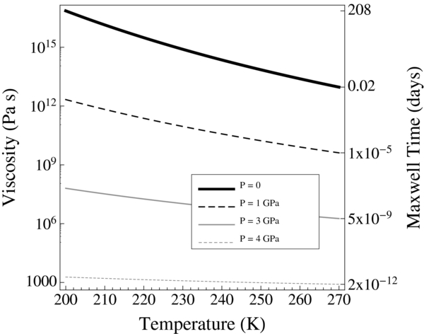
Figure 2. Viscosity for ice as a function of temperature and pressure, using parameters for Ice Ih. Note how the negative activation volume for ice (see the text) causes viscosity to decrease with greater pressures. Very low viscosity results at moderate pressures here (10 Pa s is the viscosity of ordinary honey) are an example of how low-pressure parameterizations of viscosity may extrapolate poorly to high pressures, leading to significant uncertainty for tidal heating calculations. Neglecting pressure dependence, the temperature variation here in ice viscosity for a plausible range of ice mantle adiabatic bulk temperatures spans the range from 1 × 10¹⁷ to 1 × 10¹³ Pa s. Corresponding material Maxwell times for a constant shear modulus of 4 × 10⁹ Pa are shown at right.
Download figure:
Standard image High-resolution imageThe compositional complexity of ice can be great, both from the phase diagram of water ice, as well as from the inclusion of multiple ice species such as CH4, NH3, and CO2. Eutectic blends of water with ammonia are often invoked as a likely mechanism for melting point depression in outer icy satellites. As with shear moduli, it is better to encompass such complexity by testing a range of candidate ice viscosities. This testing method has the additional benefit of reducing cases, since a very large range of temperature and compositional realities may eventually lead to the same viscosity, a handful of tests over the full viscosity range may instead then be reverse-mapped back to a heavily degenerate range of possible material causes.
A common central value for ice viscosity for outer moons is 1014 Pa s (Poirier et al. 1981; Goldsby & Kohlstedt 2001). The temperature-only-dependent range of Equation (5) in Figure 2 is 1 × 10¹⁷ to 1 × 10¹³ Pa s, and we therefore tested a range of values at least two orders of magnitude around a baseline of 1 × 10¹⁵ Pa s, with low values best representing compositional impurity, and higher values better representing cold ices.
4. RESULTS
4.1. Earth Analog Planets
Before extending an Earth model toward a super-Earth model, we first seek to establish and characterize a reliable multilayer Earth model. In previous work we have studied homogeneous tidal models of extrasolar Earth mass planets. Thus it is also of central value to investigate the degree to which a range of improved multilayer Earth models alters the outcome of tidal heating.
We find that an essential feature required to reproduce an Earth-like Re(k2) value of around 0.299, is a high value for the shear modulus of the silicate mantle. A typical value for the rigidity of surface rocks is 5 × 10¹⁰ Pa. For the deep interior, seismic velocity studies provide the parameter β = (μ/ρ)1/2, which may be inverted to determine estimates of μ given an estimate for the density. Lower mantle densities are expected to vary in the range from 5560 to 4380 kg m−3. A nominal value of 4600 kg m−3, coupled with an outer core density of 10,200 kg m−3 and inner core density of 12,000 kg m−3 leads to a nominal ∼1 ME total mass, and to shear moduli in the range from 1.6 × 10¹¹ to 2.4 × 10¹¹ Pa. An adopted value of μ = 2.25 × 10¹¹ Pa reproduces the expected Re(k2) = 0.299 for such a three-layer model.
For a four-layer model, we divide the mantle into an upper and lower layer at the 670 km depth mark. Using an upper mantle estimated density of 3900 kg m−3, a lower mantle density of 5000 kg m−3, upper mantle rigidity of ∼7 × 10¹⁰ Pa (from β of the upper mantle), increases the lower mantle rigidity required to achieve the expected Re(k2) up to 2.55 × 10¹¹ Pa. Regardless of these specific values, the primary point is that using a surface rigidity of ∼5 × 10¹⁰ at depth can lead to unrealistically high Re(k2) values of ∼0.6–0.7.
To model the continuous variation of properties within the Earth we implement a more detailed model using the Preliminary Reference Earth Model (PREM; Dziewonski & Anderson 1981). This model includes 33 layers, at roughly 200 km steps, and resolves Earth's crust, Low Velocity Zone, Upper Mantle Transition Zone, and D'' layers. For computational reasons the liquid outer core is still treated as one layer with an average bulk density. Following PREM, β in the lower mantle lies in the range 5945.1 to 7264.7 ms−1. Mapping these β values against the range of densities leads to shear moduli from 1.5 × 10¹¹ Pa to 2.9 × 10¹¹ Pa, all much greater than the surface value of 5 × 10¹⁰. Repeating this exercise for the upper mantle yields β = 5570.2–4491.0 ms−1. Because viscosities are not resolved by the seismic input data of PREM, in Figure 4 we test both a version of PREM with constant viscosities throughout the mantle, as well as a model with viscosities adapted from post-glacial rebound studies (Mitrovica & Forte 2004).

Figure 3. Pressure in a simplified ice–silicate hybrid super-Earth, with a 1 ME silicate/iron core of uniform density below a mantle of homogeneous ice, demonstrating the approximate range of pressures of interest for use in Equation (5) for the estimation of ice viscosities.
Download figure:
Standard image High-resolution imageFor the model and forcing range of primary interest, the selection of viscosity has a weak interaction with Re(k2), but is the principal control of energy dissipation via Im(k2). In Equation (1), −Im(k2) is effectively used as a replacement for Re(k2)/Q. Thus we seek viscosity values which bring a baseline Earth model's −Im(k2) close to that required to achieve a reasonable global effective Qeff value. This, however, is complicated by the strong frequency dependence of Im(k2), and on the fact that we are modeling the solid tidal dissipation of worlds, while the Q of the Earth from lunar retreat rates, Q ∼12, is mainly controlled by wave activity in Earth's surface water oceans. Even when we include water oceans in models in this work, we do so for their decoupling impact on layers, and we are not including wave dissipation or dissipation due to flow in or around specific geometries (Tyler 2008; Chen et al. 2014). The quasi-static contribution of water oceans to dissipation is otherwise negligible. The Q value for a dry Earth is unknown. There are two forms of dry in this context: ocean-free, and free of large-scale hydration in mantle minerals. A planet with little or no mantle mineral hydration may be highly viscous, as H2O can lower viscosities by several orders of magnitude (O'Connell & Budiansky 1977; Hirth & Kohlstedt 1996). For ice–silicate super-Earths, however, this is unlikely, given that a large ice mantle implies a high water fraction to begin with, thus we are interested in a Q for a baseline iron-rock core to these hybrid worlds that is free of the dissipation contribution of a surface water ocean, but is not altogether dry mineralogically. Q = 100 is often used in the literature as a dry 1 ME planet value, and the authors have used Q = 50 previously as a compromise for ocean free but still hydrated 1 ME worlds.
Bulk viscosities around 1 × 10²⁰ Pa s for the rigidity model previously cited, at a period of 30 days leads to Qeff = 1445, and at P = 300 days to Qeff = 145. Values for silicate mantle viscosity around 1 × 10²¹ Pa s typically push Q values above 10,000 as in Figure 5. At a 30 day period, bulk viscosities of 1 × 10¹⁹ Pa s can lead to Qeff = 149, 5 × 10¹⁸ Pa s to Q = 75, and 1 × 10¹⁸ to Q = 15. As seen in Section 4.2, as soon as an ice mantle is applied to a world, it is the ice viscosity and not the silicate viscosity that dominates the planetary tidal result.
In Figure 4 we model multiple variations in Earth structure. In each case the total dissipation is reported in the legend, and is a function of the applied e = 0.1, P = 30 days, and 1 MSol orbital model. Case 4A is a homogeneous model, set to the average bulk density of the Earth, with a shear modulus of 5 × 10¹⁰ Pa and viscosity of 1 × 10²¹ Pa s, following previously published baseline homogeneous Earth analogs in Henning et al. (2009). In homogeneous cases generally, dissipation is maximum in the mid-mantle, finite at the surface, and zero at the core.
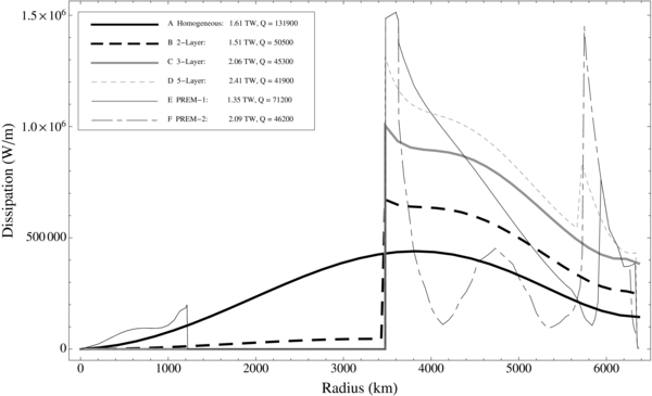
Figure 4. Tidal Dissipation for several Earth models. Case A: Homogeneous with properties of the bulk lower mantle. Case B: Solid iron core overlain by a homogenous mantle. Case C: Solid and liquid iron core overlain by a homogeneous mantle. Case D: 5-layer model with inner/outer core, upper/lower mantle, and lithosphere. Case E: PREM model with viscosities adapted from Mitrovica & Forte (2004). Viscosity maxima translate into dissipation minima. Case F: PREM model with viscosities held constant but densities and shear moduli varied continuously. Note in both PREM cases the strong dissipation in the D'' layer near the CMB. Total dissipation for each case, with e = 0.1 and P = 30 days, is reported in the legend. The smallest total dissipation is produced by the homogeneous case. The relative tidal contribution of the upper and lower mantle is a strong function of the shear modulus and viscosity contrasts between these layers. The baseline bulk viscosity is 1 × 10²¹ Pa s, with local parameters and viscosity modifications described in the text.
Download figure:
Standard image High-resolution imageNote that text references to lettered Cases in figures are prefixed by figure number to help reduce confusion due to the large number of possible cases to be shown.
In Case 4B, only a solid core and solid mantle exist, to model a simple two layer world, equivalent to a highly evolved Earth where the full core has crystallized. A liquid outer core will decouple the inner core from major tidal flexure, such that inner core dissipation is generally weak, and the viscosity selected for the inner core is of low importance. When the solid silicate and iron layers are directly coupled, the iron viscosity is of central importance. Low values around 1 × 10¹⁷ Pa s used elsewhere lead to core dissipation dominating the response by a full order of magnitude. However, since the viscosity of such an iron core is highly uncertain, especially due to the uncertain geotherm of such a high age world, we instead plot in Figure 4 a case where the viscosity of both the iron and mantle are matched at 1 × 10²¹ Pa s each, in order to detect the difference due to the density and shear moduli otherwise hidden by a viscosity contrast.
Case 4C includes a liquid outer core where dissipation is negligible. This decoupling allows greater flexure of the mantle and thus greater dissipation. Inner core viscosity is switched to 1 × 10¹⁷ Pa s in this case, while mantle viscosity remains at 1 × 10²¹ Pa s. Case 4D begins to approach a realistic Earth model, with an inner and outer core, upper and lower mantle, and low dissipation lithosphere.
The final two Cases 4E and 4F invoke the PREM model through 33 material layers where density and shear modulus vary continuously. The PREM model includes the D'' layer at the core-mantle boundary (CMB), which is found to exhibit high dissipation due to its own low strength blending with the natural maxima of dissipation at the CMB from Cases 4C and 4D. Extra layers were added at this location to enhance resolution. Tidal enhancement in the upper mantle and attenuation in the lithosphere for each PREM model is similar in form to Case 4D where properties had remained constant. The PREM model does not describe viscosities with depth, therefore Cases 4E and 4F test two viscosity models. In Case 4E, viscosities are roughly based on a synopsis of models from Figure 1 of Mitrovica & Forte (2004), where high viscosity occurs both at high depth due to high pressure, and at shallower depths due to lower temperatures, with lower values in the D'' region, mid-mantle, and upper mantle. The modeling here is not intended to be exact, but to illustrate the impact of such viscosity variations on tidal output. In Case 4F, constant viscosities of 1 × 10²¹, 1 × 10²⁰, and 1 × 10²¹ are applied through the lower mantle, upper mantle, and lithosphere, such that the impact of the PREM gradients in density and shear modulus relative to Case 4D can be seen.
Figure 4 does not include a model with a very weak asthenosphere or magma ocean (Tonks & Melosh 1993; Elkins-Tanton et al. 2003; Elkins-Tanton 2008), however, such models were also tested. Inclusion of a magma ocean just below the lithosphere often has negligible impact on the dissipation of lower layers, and the high rigidity of the lithosphere typically continues to generate negligible heating despite this decoupling. The primary impact of magma ocean inclusion is therefore the simple removal of upper mantle dissipation throughout the volume assumed to instead be liquid. Inertial effects, waves, and tidal flow (Tyler 2008) in a magma ocean, not modeled here, may however contribute in a similar manner to Earth's water ocean.
The primary result from Figure 4 is that non-homogeneous cases often produce tidal dissipation greater than the homogenous model, and very rarely produce less. Further enhancement may occur with large weak asthenospheres as in Figure 5. Enhancements by a factor of ∼1.25–1.50 are common. This occurs for two main reasons: first, including a liquid outer core allows greater tidal flexure, and second, more detailed models typically allow inclusion of local low viscosity zones. These effects often dominate over the reduction in heating caused by the removal of the liquid outer core volume from contributing to global heating. Even when low viscosity zones are small compared to overall planet volume, their dissipation typically dominates, similar to the expected dominance of the asthenosphere of Io (Segatz et al. 1988). The relative shape of depth profiles for the above cases at P = 2 or 365 days are similar to those in Figure 4, despite dramatically higher/lower overall magnitudes. At P = 3 days, total dissipation for Cases 4A–4F are: 96, 185, 281, 295, 172, 247 TW, or enhancements by factors of ∼1.8–3.1, with all multilayer results higher than the homogeneous case. Values for alternate eccentricities or host masses may be scaled using Equation (1).

Figure 5. Maps of tidal surface heat flux for three multilayer Earth models with varying upper mantle viscosity. Top row: upper mantle viscosity = 1 × 10¹⁸ Pa s. Middle row: 3 × 10¹⁸ Pa s. Bottom row: 1 × 10¹⁹ Pa s. Viscosities are selected to show the transition region of observable flux from six minima to two minima. Right panes show dissipation as a function of depth, with upper mantle heating decreasing as viscosity is raised. Core heating is negligible. Lower Mantle viscosity = 1 × 10²⁰ Pa s. Densities and shear moduli given in the text. Global response, top to bottom: W = 0.69 TW (Qeff = 600), W = 0.40 TW (Qeff = 1047), W = 0.29 TW (Qeff = 1415), each at 30 days period and e = 0.1 with a 1 MSol host.
Download figure:
Standard image High-resolution imageFigure 5 shows the distribution of tidal heat for a multilayer Earth, both in depth and across the surface in latitude and longitude, with a focus on variations in asthenosphere viscosity. Moderately low viscosity silicate asthenospheres generally attain the highest tidal response. Upper mantle viscosities are selected here to show the transition between two common surface patterns. Densities for this model are 12,000, 10,000, 5000, 3900, 2600 kg m−3 for the inner core, outer core, lower mantle, upper mantle, and lithosphere. Shear moduli are: 1.5 × 10¹¹, 0, 2.5 × 10¹¹, 7 × 10¹⁰, 5 × 10¹⁰ Pa. The inner core viscosity for this model is 1 × 10¹⁶ Pa s and the lithosphere viscosity 1 × 10²¹ Pa s. The top left panel of Figure 5 is remarkable as it is the inverse of the asthenosphere dominated six-lobed pattern found for Io (Segatz et al. 1988). We find that the mid-valued viscosity contrast pattern (middle panels) is most common for an Earth analog exoworld.
Variation of the orbital period has minimal impact on the pattern of the surface distribution when outside of the transition range where upper and lower mantle heat rates begin to converge, but can dramatically change the pattern when this range is encountered. For most models, a period of 3 days leads to an upper mantle dominated pattern, while a 300 day period is less well tuned, causing a decrease in heat from lower viscosity zones, switching behavior to a lower mantle dominated pattern. Patterns of surface heat flux are often transitional for periods from 10 to 50 days.
4.2. Ice–Silicate Hybrid Planets
We may roughly divide ice–silicate hybrid exoplanets into those which may contain internal liquid water oceans, and those which do not. Water oceans are expected to be a shallow or surface phenomenon (Fu et al. 2010), while in contrast, ice mantles may plausibly exist with very large thicknesses, up to the limit of the ∼2 RE (∼12,700 km) ice mantle thickness expected for 3.8 RE Neptune. In practice we test the impact of internal water oceans within ice mantles of up to 3000 km thickness, and assume that above this ice thickness, basal or internal oceans become unlikely and interest lies mainly in the physics of the solid ice layers fully coupled to solid silicates below. We first consider ice-only mantles, and then consider ice mantles in the presence of water oceans. In order to focus on bulk structural questions first, in this section we report upon ice mantles with constant viscosities and shear moduli, however, in Section 5 we consider gradations in material properties.
Figure 6 shows the distribution of tidal heating with depth for a range of ice–silicate hybrid planet models. Two key results are found: first, that ice–silicate tidal systems are highly insensitive to the choice of silicate/iron core model, and second, that the primary controls on the magnitude of total tidal heating (and thus effective Q values) are the viscosity of ice used, and the presence or absence of any decoupling water ocean.
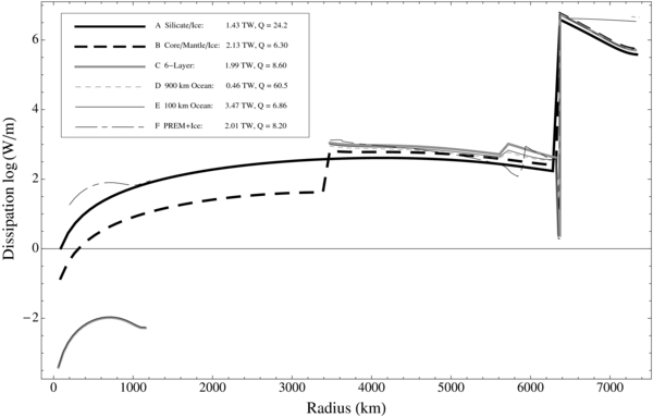
Figure 6. Tidal dissipation vs. depth for ice–silicate hybrid super-Earth models. For plausible ice surface conditions, the orbital environment is changed from Figure 1, to a 60 day orbit around an analog of 55 Cnc with Mpri = 0.9 MSol, Lpri = 0.54 LSol, with e = 0.1, an albedo of 0.87, and blackbody surface temperature ∼270 K. Note logarithmic vertical axis. Case 6A: 1000 km ice atop a homogeneous 1 ME silicate core. Case 6B: Solid iron core, silicate mantle, 1000 km ice. Case 6C: Solid and liquid iron core, lower and upper mantle, lithosphere, and ice. Case 6D: Same as Case 6C with but with a 100 km water ocean decoupling a 900 km ice shell above. Case 6E: Same as 6C with a 900 km water ocean and 100 km ice shell. Case 6F: PREM model with ice mantle above. Total dissipation and effective Q values shown in legend. Variations in silicate/iron structure follow Figure 4, but have negligible impact on total dissipation due to the very strong viscoelastic response of ice. The primary controls on overall dissipation are the viscosity of ice and the existence and thickness of a decoupling water ocean (see the upper right corner). Note how total dissipation is comparable to Figure 4 despite a significantly more distant orbit and smaller host star.
Download figure:
Standard image High-resolution imageIron-core mass fraction changes are found to have only a very minor impact on overall results due to the dominance of ice material properties on the tidal response. High iron core fractions are similar in impact to higher silicate densities in the sense that the entire iron-silicate component of the planet acts as an aggregate core. Switching from a liquid iron outer core, to an all-solid or all-liquid iron core has limited impact beyond planets with very thin ice mantles for the same reason.
Surface maps of ice-hybrid super-Earth tidal heat flux integrated over one orbit and summed over depth are shown in Figure 7. Ice mantles in general often produce response patterns in latitude and longitude similar to the asthenosphere-dominated response described in Segatz et al. (1988) for Io. In general, cases involving any low viscosity material of modest depth overlying a large depth of high viscosity material generate six-lobed global maps of dissipation with maxima at or near the equator. In contrast, when dissipation is optimal in a material which spans the majority of the body, as in the mantle-dominated cases of Segatz et al. (1988) for Io, or any homogeneous planet model, then tidal heating is maximum at the poles with two broad minima at the equator. Such polar maxima for tidal heat production may roughly be understood to arise from the dominance of shear stress terms in the overall system response.

Figure 7. Demonstration of how ice mantle thickness is the primary control on the pattern of tidal surface heat flux. Ice mantle above a 1 ME silicate/iron core, with ice thickness varying from 100 to 6000 km. Ice viscosity = 1 × 10¹⁵ Pa s. At ∼200 km ice thickness and above, tidal dissipation in the ice overwhelms the background pattern of silicate/iron core heating. Cases of ∼3000 km ice shell thickness generate patterns of 6 maxima lobes akin to the asthenosphere-dominated pattern of Io first described by Segatz et al. (1988). Even further concentration of heating into the upper half of the planet transitions further into a pattern of 6 minima, as in the top row of Figure 5 (an ice free Earth). Both thick and thin cases with water oceans (Cases 6D and 6E) generate patterns nearly identical to the 6000 km ice case here without an ocean, but with different total heat magnitudes. Orbital environment the same as in Figure 6.
Download figure:
Standard image High-resolution imageA new situation occurs in Figure 7, panel 5, where the thickness of the low viscosity material with the more optimal tidal tuning is no longer a thin top veneer, but instead approaches one-third of the body radius. In these situations the pattern of dissipation evolves beyond the six lobed case of a thin active upper layer, and heat becomes further concentrated to a belt around equator. When this layer approaches half of the body radius, as in Figure 7, panel 6, or the top panel of Figure 5, the pattern transforms to one of six minima, or the inverse of Figure 7 panel 3. Note that previous work has described the range in outcomes from Figure 7 panels 1 to 3 as endmembers of the solution space, however Figure 7 demonstrates that these patterns are in fact part of a much larger system of solutions.
The transition in surface patterns shown in Figures 5 and 7 is partly explained via Figure 8, which demonstrates how tidal heating as a function of depth systematically changes in an low-viscosity upper layer of increasing thickness. Homogeneous ice mantles of viscosity 1 × 10¹⁵ Pa s, density 1000 kg m−3, and shear modulus of 4 × 10⁹ Pa are shown from 400 km to 10,000 km thickness. In all cases the silicate/iron core is a homogenous solid with constant density set to match 1 ME, because of the demonstration in Figure 6 that ice mantle tidal results are insensitive to silicate/iron core structure, especially for ice mantles above a few hundred kilometers thickness. Again, an orbit of e = 0.1, P = 60 days at an analog of 55 Cnc is used, thought the phenomenon highlighted here is not sensitive to these choices, only the total heat magnitudes are.
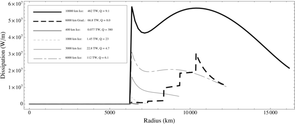
Figure 8. Depth profiles of tidal heating for super-Earth planets with high ice mantle thicknesses, approaching ∼2.5 RE and the mini-Neptune transition range. As ice mantle thickness increases, the heating maxima transitions from a basal focus to a mid-layer location. While not shown due to not representing any realistic planet structure, if the ice (or any tidally susceptible material) mantle thickness were increased further to consume the full planet radius, the tidal heating profile would transition all the way back to the form for a homogeneous world from Figure 4 Case A. Included here is one example of how gradations in layer properties alter results: with a 6000 km ice mantle and five steps in viscosity from 1 × 10¹⁵ Pa s (surface) to 1 × 10¹⁷ Pa s (base), in density from 1000 kg m−3 to 1200 kg m−3, and constant shear modulus of 4 × 10⁹ Pa. Note how tidal heating is dominated by the size and properties of only the lowest viscosity component of any such gradational layer. Orbital environment the same as in Figure 6.
Download figure:
Standard image High-resolution imageAs an ice mantle grows in thickness, it transitions from a profile where tidal heating is maximum at the base of the layer, to a form where a mid-layer maxima rises to dominate. Note that the mid-layer feature need not actually exceed the basal maxima in order to dominate the result, because the feature's widths also matter when total power is integrated with depth (Note that in units of W m−1, the higher importance of upper layers due to their greater volume has already been taken into account). Results in Figure 7 may thus be reinterpreted as follows: at tice = 100 km, silicate-core features remain the dominant surface expression. At tice = 400 km, ice heating features dominate, with a basal maxima in layer heating leading to a six-lobed surface pattern. At tice = 3000 km, the six-lobed basal heating feature begins to be replaced by the mid-layer maxima, with the net result of an equatorial focusing of heat. At tice = 6000 km, the mid-layer maxima in heating fully dominates surface expression. Above this thickness the top layer is sufficiently thick that the surface expression begins to return to the form of a homogeneous body, with the effect of any small poorly coupled core eventually vanishing in importance. We find this pattern cycle is common for any high tidal susceptibility material placed atop a low tidal susceptibility core, and considered in terms of increasing thickness (e.g., it also applies to a growing silicate asthenosphere).
The origin of the multiple tidal heating surface patterns which may occur has no simple origin, and arises from the summation of dissipation maps which can be decomposed by tensor product component as in Figure 9. Such component maps may also be considered for the instantaneous work in time at each orbital position, as well as for the stress and strain tensor terms themselves. Individual maps vary with depth and forcing frequency, such that their collective sum weighed by varying magnitude in depth becomes more difficult to visualize. For two-layer worlds, Beuthe (2013) discusses the origin and range of tidal heating patterns in detail. In general, shear terms in stress lead to greater polar heating, and are dominant for the typical mid-layer maxima of homogeneous planets or extremely deep asthenosphere-like layers. The basal maxima typical of the CMB or any ice–silicate transition contain a more even mix of shear and normal stress terms, leading to more equatorial final expressions of surface heat.

Figure 9. Dissipation for an ice hybrid world decomposed into directional components of internal work, in W m−3. It is the weighted combination of these patterns varying over depth that gives rise to the total surface pattern observed, after integration with depth. Note that in units of power per unit volume, heat rates that lead to polar maxima of surface flux are distorted by rectangular projection, however, the general trend that normal stress driven components lead to more equatorial heating and shear components lead to more polar heating remains evident.
Download figure:
Standard image High-resolution imageThere is sufficient systematic variation in tidal surface patterns based on internal structures, that they may help to constrain the interiors of observed exoplanets in the future. Observations are already able to map large-scale hemispheric temperature dichotomies and offsets in temperature maxima from the substellar point for Hot Jupiters (Knutson et al. 2007; Cowan & Agol 2008). Studies suggest that mapping Earth analog solid surfaces due to rotation in inclined orbits may be plausible with upcoming technology, including both 1D maps (Fujii et al. 2011), and 2D maps (Kawahara & Fujii 2010, 2011; Fujii & Kawahara 2012). To observe the heat pattern of a super-Earth due to its internal tidal activity would require a planet orbiting close a very low luminosity host, ideally in a transiting configuration which allowed a tight constraint on orientation of the equator. Large moons far from host stars may be advantageous targets, and Peters & Turner (2013) have discussed the possibility of directly imaging the tidal signature of such hot exomoons. A rare ideal case would include periodic eclipse of one pole only, allowing for a polar vs. equatorial relative measurement. If the lightcurve of a tidal planet could be shown to have four brightness maxima in longitude, this would indicate a thin tidally active upper layer, but only two maxima would point toward a tidally active layer spanning the majority of the radius. Liquid oceans and atmospheres however will redistribute heat and may blur such effects. Yet even with the complexity evident in observing Io, or the lack of global distribution of heat on Enceladus, patterns of tidal enhancement have helped to constrain interior models (Kirchoff et al. 2011; Hamilton et al. 2013), and any opportunity to constrain the interior of a world (Ragozzine & Wolf 2009) in another starsystem will be significant.
Figure 8 also includes the total heat output and effective Q values for worlds with deep ice mantles. Such total heat values present a mixed picture. On one hand, values are mostly small compared to the ∼44 TW heat output of the modern Earth (and therefore the likely order of magnitude for non-tidal heat output from such world's silicate/iron cores even prior to tidal heating). On the other hand, eccentricity values well above e = 0.1 are observed in exosystems, and tidal heat (even for complex multilayer worlds) will scale as e2. Similarly, many hosts smaller and less luminous than 55 Cnc exist, providing opportunities for ice mantles at shorter periods, and tidal heating strongly scales as the fifth power of mean motion, n5. Therefore, only a small increase in albedo, a small decrease in host luminosity, or simply the allowance of a thin liquid water surface ocean followed by clathrates and solid ices after only a few 100 km's depth can all lead to far greater heating. Lastly, Figure 8 uses a conservative ice viscosity of 1 × 10¹⁵, but lower values remain plausible due to issues discussed in Section 3.3.
The first two cases shown in Figure 8 illustrate an important point regarding Q values. For the same orbit, the first case with a 10,000 km ice mantle and Qeff ∼ 9 produces nearly ten times the total heat in Watts compared to the second case with a 6000 km ice mantle and Qeff ∼ 8. This occurs due to changes in the planetary Love numbers, and highlights the reason why the value −Im(k2) for a given planet is a significantly better scalar measure of the world's tidal susceptibility than a Q value alone. Recall that −Im(k2) replaces the ratio k2/Q in the viscoelastic form of the classical tidal equation. For this reason, later figures here report −Im(k2) values, which may be converted to effective Q values via: Qeff = Re(k2)/− Im(k2). In later use, we generally omit the subscript eff, as all forms of Q values are already only a proxy for susceptibility to tidal heating, and only W(n, T) for a given planetary case is the final measure.
The Love and Shida numbers for simple ice–silicate worlds with ice mantle thicknesses up to 10,000 km are shown in Figure 10. Near and above this thickness, large gas envelopes are expected to alter results, unless unusual envelope stripping has occurred. Results are separated between the real and imaginary components of each Love number. In the Fourier model of viscoelastic tides, real components generally characterize elastic behavior, while imaginary components characterize energy dissipation. k2, representing the gravitational response, is directly applied to tidal heat predictions. In a homogeneous case, −Im(k2) may characterize the entire tidal heat response, and in these cases where the ice mantle dominates dissipation, it becomes a reasonable proxy for total tidal heating. The displacement Love number h2 and Love–Shida number l2 may be interpreted to signify the magnitude of radial and tangential surface displacements respectively. While l2 is most properly referred to as the Shida number or Love–Shida number, for clarity below we do refer to the three related values k, h, and l by the common aggregate term Love numbers.

Figure 10. Surface Love and Shida numbers for ice–silicate hybrid planets with ice mantles up to 10,000 km at multiple orbital periods. Cases 10A and 10B: silicate mantle with constant properties extended to high thickness, for comparison to ice results, at forcing periods of 3 days and 300 days. Cases 10C–10G: Ice mantles with constant properties for orbital periods of 3, 15, 30, 150 and 300 days. At longer periods tidal resonance (mainly expressed via Im(k2)) occurs primarily for ice mantles below 2000 km thickness. At high thickness, all cases monotonically move toward but do not yet approach the strength free hydrostatic limits in Re(k2) and Re(h2). Models with graded ice density at high pressures will shift toward silicate-only curves in real components. Models with gradations of higher viscosity at high pressure shift toward silicate-only curves in imaginary components. In all cases mantles rest atop a 1 ME iron-silicate core and are insensitive to eccentricity and host mass. The strongest potential for high tidal activity lies with high thickness ice mantles with forcing below 15 days.
Download figure:
Standard image High-resolution imageFigure 10 demonstrates a material tidal resonance with ice layer depth, which typically occurs between tice = 1000–2000 km. Above these thicknesses, Love numbers grow or contract monotonically with increasing depth, with little change in magnitude for imaginary terms. Re(k2) and Re(h2) shift steadily upward for deep mantles but remain far from their hydrostatic limits of 3/2 and 5/2, respectively. Such limits are more typical of gravity dominated gas giants. Re(k2) and Re(h2) decrease relative to a 1 ME core for ice depths below 2000 km, as the low density of ice allows the aggregate objects to briefly appear more strength dominated. Orbital period has a strong impact on the depth and especially the depth range that causes tidal resonance. Peak magnitudes in imaginary components remain similar across the whole period range shown. In particular, note how the full high resonant −Im(k2) response may occur across the enormous ice thickness range from about 3000–10,000 km at short periods, while at long periods an ice mantle must be perfectly tuned by chance to around 1000 ± 100 km in order to experience a similarly high response.
While silicate-only mantles of this thickness are unrealistic, they are shown for comparison with ice results and represent a high-density, high-viscosity limit, which high pressure ice may approach. We plot constant density curves to help bound the behavior of the physical system. Full models of the interior from an equation of state and thermal flux model will, in addition to adding numerous new poorly constrained degrees of freedom to the system, be fully temperature dependent, and require iterative solutions with tidal heat flux as discussed in Section 3.3. As tidal heating depends far more strongly on viscosity than on density, the benefit of a full equation of state approach is also lessened when our goal is determining heat outcomes. Parameter gradations are discussed in more detail in Section 5.2, with results showing that low pressure upper ice levels are the primary control on dissipation.
While this paper does focus on questions of heating, very high surface displacement predictions are typical in strong tidal forcing cases, and displacement is significantly greater in low rigidity (4 × 10⁹ Pa) ice than in any underlying (5 × 10¹⁰ − 11 Pa) silicate. For example, lateral surface movements of ∼4 km, and radial displacements of ∼1 km may occur for a 4000 km thick ice mantle in a three-day period. This corresponds to surface strains of θθ ∼ 0.005, rr ∼ 0.003, ϕϕ ∼ 0.002, and θϕ ∼ 0.001. In general, the high strains experienced for such worlds suggest the possibly of extreme faulting, perhaps analogous to tidal features on Europa (Hurford et al. 2005, 2007b). The opening of faults by the tidal cycle may also induce periodic eruptions of volatiles as on Enceladus (Hurford et al. 2007a) and perhaps Europa (Roth et al. 2014), the timing of which may in the future be detectable through careful primary or secondary eclipse transit spectroscopy (Kaltenegger et al. 2010).
5. DISCUSSION
5.1. Effect of Water Ocean Position and Size
Fu et al. (2010) model the thermal structure of large ice mantles in detail. For the near surface of 2, 5, and 10 ME super-Earths, they find a complex range of outcomes may arise from the interaction of the geotherm with the ice Ih, III, V, and VI portion of the phase diagram in the upper ∼60 km of planets. Both the presence or absence of a liquid ocean below a largely ice Ih crust is plausible, due to the unique notch in the liquid-solid phase boundary in the water phase diagram in this pressure regime at temperatures near 250–280 K, and is largely controlled by internal heat flux. Naturally, the surface temperature, itself a strong function of atmospheric state and solar flux, is the primary control on whether or not such an ocean extends up to the atmospheric interface as well. Since our current model assumes a solid surface, we focus on worlds where all water oceans exist below some amount of solid ice. These models are expected to also be close approximations of the total tidal dissipation and internal deformation of worlds with thin or modest liquid water oceans at the surface. In such an extended application, surface Love numbers here for the solid top case clearly do not represent the shape of a thin-to-modest liquid ocean's top surface that might be observed, but do approximate the shape of the base of such a layer.
For surface temperatures above 273 K, it is somewhat difficult to achieve a solid ice surface due to pressure alone. At 274 K, ∼6 kbar or 630 MPa is required, which would require an unrealistically large gas envelope for a 1.4 ME world. Therefore, our analysis is limited to cases where a surface ocean, if present in cases of Tsurf ⩾ 273 K, will be thin enough that Love numbers for the layer system beginning at the first solid interface are a close approximation of the body as a whole. 630 MPa is for example achieved under almost exactly 100 km of water for a 1.4 ME world.
Beyond this, the criteria for a solid top layer is best achieved in cold environments. This is somewhat incompatible with strong tidal forcing of planets near to their host stars. Therefore, the analysis here is most useful for ice–silicate hybrid worlds encircling dim host stars, such as L and M-dwarfs, white dwarfs, neutron stars, or pulsars. Similarly, such a combination of strong tidal forcing and cold surface temperatures is achieved for larger moons of Jupiter and super-Jupiter class worlds, as well as the tidal evolution of binary terrestrial planet systems.
Water oceans may also exist at significant depths due to rising temperatures. The basal pressure of an ice mantle of ∼3000 km thickness, atop an Earth-mass core, is around 19 GPa, which for temperatures between ∼250 K to 750 K places ice in the ice VII phase. Above 750 K, supercritical liquid water is still possible at this depth (where all liquid above 647 K is in the supercritical state). The majority of a 3000 km ice mantle should participate in convection, except for worlds with unrealistically small silicate cores or worlds vastly older than the solar system timescales of interest here. The adiabatic geotherm in a convecting ice layer is typically shallow, making temperatures much beyond this range, even at depth, less likely. Eutectic melting point depression in ammonia-water systems has also been suggested as a common planetary mechanism for liquid ocean maintenance, and may allow for a complex diversity of liquid layers, including perched oceans with solid ices above and below.
The density of Ice VII in this deep and warm regime is still marginally well represented by ∼1000 kg m−3. Below ∼400 K the density climbs above 1100 kg m−3, but only reaches 1200 kg m−3 when as cold as around 200 K. Therefore, our focus may remain on viscosity variations and not density variations.
Figure 11 shows tidal surface Love numbers for ice–silicate hybrid super-Earth planets, showing variations as an ice mantle up to 3000 km thickness is added above a baseline Earth model of 1 RE, 1 ME, with a solid iron inner core, liquid outer core, and uniform silicate mantle. The maximum planet mass in these plots is 1.39 ME, with a total radius of 1.47 RE. A forcing period of P = 30 days is used. Note the log scales for imaginary components. In Case 11B a solid ice layer of density 1000 kg m−3, shear modulus 4 × 10⁹ Pa, and viscosity 1 × 10¹⁴ Pa s, is applied. This solid-only case leads to significant variations in h2 and l2 as a function of ice mantle thickness, and the highest dissipative response through −Im(k2). In Case 11C this same ice mantle is separated from the silicate below by a 10 km thick water ocean. This greatly reduces the dissipative (imaginary) response, while h2 and l2 switch to monotonic behavior because they no longer reflect a transition from dominance by the silicate to dominance by the ice. Re(k2), which depends largely on the density structure of layers, is minimally changed. In Case 11D this decoupling ocean is enlarged to 500 km. This has negligible impact on the dissipative response of the planet, and has only a minor impact on real valued components through the additional mass. Case 11E tests the concept of a perched water ocean, by placing a 10 km water layer at the midpoint of the given ice thickness. This significantly reduces the dissipative response, but has a real response nearly identical to Case 11C. Case 11F places a 10 km water ocean below a 20 km surface ice shell, with the bulk of the ice below both, directly attached to the silicate mantle. The result is similar to Case 11E but with less reduction in dissipation. For comparison, in Case 11A the silicate mantle is extended to match the overall radius of the ice-hybrid world, leading to a very low dissipative response, and a gradually more hydrostatic real-valued response. Overall this indicates that ocean presence is critical, ocean thickness negligible, and ocean position important mainly for the magnitude of dissipation.

Figure 11. Tidal surface Love numbers for silicate and ice–silicate hybrid worlds, testing variations in structure and ocean position at P = 30 days. Solid ice mantles with no ocean have the greatest potential for tidal heating, while adding oceans of any size can greatly reduce the tidal heat response (via −Im(k2)), even while often increasing surface deformation (via Re(h2) and Re(l2)). The all-silicate Case 11A is included only for comparison with ice mantles as a high-density high-viscosity limit. Note log scale for imaginary components. −Im(h2) and −Im(l2) included in this figure only, to show their general similarity to the behavior of −Im(k2). All cases contain a 1 ME core. See the text for model details.
Download figure:
Standard image High-resolution imageFigure 12 shows the effect of varying the orbital forcing period on the surface Love numbers of ice–silicate hybrid super-Earths. Baseline Earth model as in Figure 11. Solid curves: Ice mantles with no water ocean, varied from a 2 to 50 day orbital forcing period. At longer periods, the peak (Re(l2), −Im(k2)), or minimum (Re(k2), Re(h2)) response of non-monotonic functions occurs at smaller ice mantle thicknesses. Dashed Curves: Ice mantles are separated from the silicate mantle below by a 10 km water ocean. Changes in real-valued components are negligible with forcing frequency, while the dissipative response (−Im(k2)) is highest at short periods. This is the opposite of the dissipative trend for the solid cases for thinner ice mantles (prior to any peak), which achieve maximum dissipation at longer periods. Note that for decoupled ice mantles, the shape of the imaginary component curves is entirely insensitive to the forcing period, and thus dissipation is always greater with greater thickness, while for solid-only ice mantles, there is generally a thickness for peak dissipation at any given forcing frequency.

Figure 12. Tidal surface Love numbers for ice–silicate hybrid worlds testing variations in forcing period in ice mantle thicknesses up to 3000 km. Solid lines: ice mantles with no water ocean. Dashed lines: 10 km thick water ocean at ice base. Note log scale for −Im(k2). Models with and without oceans converge at high tice or long periods. While oceans almost always decrease total heating (via −Im(k2)), solid worlds switch ordering of strong vs. weak dissipation in both period and thickness, but for worlds with oceans, short period cases and high thickness cases always have greater heating. In a few thin-shell cases, worlds with oceans experience more heating than all-solid worlds. See the text for model details. Note that period variations are sensitive to rheology choice, and the Maxwell rheology used may have more frequency dependence than materials with compositional inhomogeneity.
Download figure:
Standard image High-resolution imageContinuous variation of ocean position was tested and found to have minor impact beyond that already reflected by base and near surface ocean position endmembers. There is some dependence of Re(k2) and Re(h2) on position, but it is weak and mainly expressed at short periods, such as P = 2 days (Note that Love numbers are a function of the planet only, and therefore apply to all host masses and eccentricities). At P = 2 days, all ocean positions lead to increasing −Im(k2) with increasing ice thickness. At longer periods, near surface oceans lead to decreasing −Im(k2) with ice thickness. At long periods, e.g., P = 300 days, even the dependence of −Im(k2) on ocean position begins to be lost, but the dependence of Re(l2) is enhanced. Near surface oceans lead to the highest ocean bearing branch for Re(l2), consistent with the idea that freedom of an outer ice shell to deform laterally without connection to the lower solid increases the overall lateral crustal deformation response.
5.2. Gradations of Ice Layer Properties
When a uniform growing ice mantle is applied to a silicate-iron core with gradations in the silicate properties using the PREM baseline, results almost exactly overlie those for a single or double layer silicate mantle model as shown in Figure 11, with the exception of slight constant offsets due to any imperfectly matched ice-free values. We find this to be true both at short and long forcing periods. Thus, the importance of such iron/silicate interior gradations is negligible in terms of surface Love numbers for ice hybrid worlds, except when ice layers are less than a few hundred km in thickness.
Of greater importance is any gradation of ice viscosities. Cold brittle ice with a viscosity up to 1 × 10²¹ Pa s has been suggested for the non-convective top layer of Europa's ice shell, yet near surface warm convective ice may have viscosities from 1 × 10¹³ to 1 × 10¹⁵ Pa s depending on composition and conditions. As with silicates, there are competing effects upon the viscosity of ice with depth: as high pressure may act to increase or decrease viscosities, while increasing temperature with depth acts to lower them. Thus, it is not immediately clear for a given composition and global heat flux which behavior may dominate, as discussed in Section 3.3.
Compared to the range of variation possible for ice viscosities, the range available for ice densities and ice shear moduli, even under high pressures in a deep ice mantle, are comparatively small. Ice density may increase by a few percent, but it will not vary over up to two orders of magnitude. Therefore Figure 13 shows models where only the viscosity is varied in the ice layer, so as to deconvolve this strong primary effect from any other more modest parameter variations.

Figure 13. Impact of gradations in ice properties. 100 day forcing period. Case 13A: Uniform solid ice, Case 13B: ice viscosity increasing with depth from 1 × 10¹³ to 1 × 10¹⁵ Pa s. Case 13C: ice viscosity decreasing with depth. Case 13D: brittle η = 1 × 10²¹ Pa s ice top. Cases 13E–13H: Same as 13A–13D but with a decoupling basal ocean. Note log scale of −Im(k2).
Download figure:
Standard image High-resolution imageIn general, ice property gradations have a major impact on outcomes, however, it is usually the uppermost layer properties which continue to dominate the response. Because the overall viscosity has changed, imaginary components experience significant changes in magnitude. A brittle top suppresses dissipation (e.g., lowers −Im(k2) values) both with and without an ocean (13D and 13H). Unlike for solid-only cases, for models with a thin ocean, both forms of a viscosity gradation (13F increasing with depth from 1 × 10¹³ to 1 × 10¹⁵, or 13G decreasing with depth from 1 × 10¹⁵ to 1 × 10¹³), will increase dissipation. Here amplification due to the lowermost layer is also activated partly due to the higher stress concentration typical at interfaces between a solid top layer and underlying ocean, as seen in Figure 4. Gradations also alter system natural frequencies, such that the ice thickness for peak dissipation or maximal or minimal deformation shifts from a pure case.
The trend for ice gradations to have high importance continues at other forcing periods. Results for a short period of three days are shown in Figure 14, and are distinctly different from patterns in Figure 13. At this short period a much greater fraction of structure cases lead to dissipation which increases monotonically with ice thickness, and overall lowers the chances that any response peak of a property lies within the 0–3000 km ice mantle range.

Figure 14. Impact of gradations in ice properties at short periods, at P = 3 days. Cases same as in Figure 13. Note the extent to which patterns shift from those of Figure 13, demonstrating the complexity of results across multiple forcing periods. For this reason, and the sensitivity of temperature structures to forcing histories, we caution that the tidal behavior of ice worlds with similar sizes and ice fractions but different orbits can yield very different tidal outcomes.
Download figure:
Standard image High-resolution imageThe most interesting gradation case occurs at long periods, where a double peak in the dissipative response appears in the case of a solid ice mantle with a brittle top. In this scenario the natural frequency of the convective ice layer and brittle ice layer are sufficiently unique to produce two visibly separate peaks, and the forcing period of 100 days in Figure 13 happens to excite both within the ice thickness range applied. This example is illustrative of a general phenomenon that may occur for high viscosity contrast layers. A similar tendency to multiple peaks does not occur for both the silicate and ice layers due to the challenge of exciting a thick deep 1 × 10²¹ Pa s layer versus the easier task of exciting such a brittle layer as a thin surface shell.
5.3. Variations with Orbital Period
Figure 15 concludes by showing the tidal behavior for selected models as functions of orbital period. Total heat, effective Q values, and circularization times following Equation (2) are shown. Again a host star mass and luminosity following 55 Cnc is used to allow colder surfaces so that direct comparisons may be made between ice and silicate worlds, however, curves in Figure 15 are nearly identical to those for a host star with a mass of 1 Msol. Silicate-iron worlds are shown in the top row, while ice–silicate worlds are shown in the bottom row. Cases are selected to highlight the role of low viscosities, magma oceans, and water oceans. Even with a conservative assumption on eccentricity, geologically relevant tidal heating is shown to extend out to ∼50–100 days in a variety of cases, with a horizontal threshold of 5 TW used to denote this approximate activity level. Geologically relevant tidal activity extends to longer periods more often in ice–silicate hybrid cases (bottom left panel), with deep-ice mantle cases (e.g., 6000 km of ice or more) constituting the longest period active worlds.

Figure 15. Tidal behavior as functions of orbital period, showing total heat, effective Q values, and circularization times. (Top row: silicate worlds. Bottom row: ice-silicate hybrid worlds.) As interiors are warmed, Earth-analog planets switch from low to high dissipation, then back again to low in very hot cases. The majority of circularization timescales are longer than our solar system age. At the same time extreme tidal heat rates ⩾106 TW do remain possible even with large magma oceans at short periods. For ice–silicate hybrid worlds, the only reliable trends are that high thickness cases are the best pathway to high tidal heating, and high melting cases are the best pathway to low dissipation. Adding near-surface oceans has minimal impact on outcomes. Adding a basal water ocean may increase dissipation at some periods but not all, depending heavily on structure and viscosity details. Altering ice viscosities or introducing ice viscosity gradations remain close to the basic cluster of results displayed. e = 0.1, and all host stars have a mass following 55 Cnc to make ice surfaces more plausible at shorter periods.
Download figure:
Standard image High-resolution image
For Earth-mass silicate-iron worlds, all structure variations tested in Figure 4 cluster close to the second curve in Figure 15 labeled 1 ME Multilayer, including both PREM variants. The most important result of Figure 15 is the change that occurs between worlds we label as Cool Dry Earths, Warm Earths, and Very Hot Earths. By Cool Dry Earths we refer to worlds without dissipation in a surface water ocean, with mantle structures and mantle viscosities similar to the modern Earth. The high viscosity of such mantles leads to very low dissipation, very large Q values, and very long circularization times. Such worlds may retain initial eccentricities for much longer than solar system lifetimes, even at short periods, given that their eccentricities are not so large as to heat them into the next Warm Earth category. This finding may help to explain some high eccentricities observed in the exoplanet population for terrestrial class planets.
A significant change occurs for Warm Earth cases, when we assume the mantle and asthenosphere viscosities of silicate material are far lower than for the modern Earth, and close to viscosities at or just above typical solidus temperatures for mantle materials. For a mantle viscosity of 1 × 10¹⁷ Pa s (e.g., high pressure, just sub-solidus) and asthenosphere viscosity of 1 × 10¹⁴ Pa s (e.g., just above solidus), tidal heating of ∼5 TW may occur out to 80 day periods at e = 0.1, to 320 days for e = 0.2, and 2000 days for e = 0.5. Solutions of ∼10,000 TW are plausible for partially melted silicate worlds out to periods of 20, 80 and 500 days for the same eccentricities. While higher order terms in eccentricity become important above this level, such moderate Warm Earth silicate worlds have the potential to maintain the heat required for a high partial melt fraction mantle across a very large range of orbital periods relevant for terrestrial planet formation. Following Figure 1, the definition of Warm Earth above corresponds to bulk layer temperatures that are only ∼300–400 K higher than the present Earth. Effective Q values plummet for Warm Earths, falling 4–5 orders of magnitude relative to a Cool Dry Earth, and well below the common assumption of Q = 100. Typical Warm Earth Q values are in the range 1–10, with values of Q = 1–2 very common for short periods. Circularization times for such worlds are far faster than their cool counterparts, a result that can help warm Earth-analog worlds to rapidly recover from high eccentricity scattering events, and reduce the number of terrestrial planets vulnerable to being lost from early active solar systems due to orbit crossings or three body encounters.
Only for the most extreme Very Hot Earths, does the opposite behavior occur, with Q values again rising back above 100, and into the Q = 1000 range. We emphasize that this is a highly unexpected result. Conventional wisdom suggests that melting in general reduces dissipation, thus extending circularization times, and making Earths vulnerable to orbital crossings and system loss for longer times. Instead, we find that the path of multilayer global heating first produces an extreme increase in dissipation, thus shorter circularization times, and only once a magma ocean consumes a very large fraction of a mantle, does traditional tidal shutdown begin. This is a uniquely multilayer effect, caused by the low viscosity warm mantle underneath a magma ocean. Here, even the imperfect viscoelastic tuning of warm lower mantle material more than compensates for the loss of active volume from magma layers. Note how even the most extreme magma ocean cases shown have lower Q values (greater dissipation) than Cool Dry Earths, again counter to the notion of tidal shutdown. Overall, all dry planet results with Q near the 20–100 level are rare, and thus the assumption of Q ∼ 20–100 is most useful for Cool Wet Earths: e.g., planets expected to strongly resemble the modern Earth in age, orbital forcing, and expected surface water ocean state.
The viscosity at which behavioral transitions occur is period dependent. A Maxwell time of 100 days is achieved for silicate material with a viscosity of around 1 × 10¹⁷ Pa s (or 1 × 10¹⁶ Pa s for 10 days). At this period, below this viscosity, the tidal response is again attenuated. For the cases containing magma oceans in Figure 15 we have tested values for the remnant solid lower mantle of 1 × 10¹²–1 × 10¹⁴ Pa s, to try to bring about the least dissipation plausible for such layers while remaining a solid. Lower mantle viscosities any closer to 1 × 10¹⁶–1 × 10¹⁷ Pa s in Very Hot Earth cases will show even less of an increase in Q. The fact that creating Very Hot Earth class results requires stretching the parameter range to this extent hints at how common Warm Earth class results will be. The relative position of Q values for each category can be viewed as an aggregate reflection of the distance from the ideal Maxwell tuning of each worlds' dominant layers: e.g., at ∼1 × 10¹⁷ Pa s, Warm Earths are ideally tuned, while Very Hot Earths at ∼1 × 10¹⁴ Pa s are still typically closer to their ideal tuning than Cool Dry Earths at ∼1 × 10²¹ Pa s. For improved rheologies beyond the Maxwell model, specific ideal tuning frequencies will vary, often with more gradual transitions between categories, but regardless of rheology the overall pattern will remain robust that dissipation is lowest for cool and hot cases, and highest for intermediate cases.
Previous analysis (Henning et al. 2009) has shown that feedback with mantle convection by the mechanism described in Moore (2003b) will cause the majority of strong tidal forcing cases to rapidly evolve into very stable tidal-convective equilibrium states at low-to-modest melt fractions. While this previous work was performed for a homogeneous mantle, the general tidal-convective equilibrium mechanism makes it very difficult for planets to reach the Very Hot Earth states with deep magma oceans demonstrated here. We conclude such states are only possible when external orbital forcing is extremely strong, such as for P ⩽ 10 days, or at longer periods e ⩾ 0.5. This means that the vast majority of terrestrial planets warmed any significant amount more than the modern Earth, are expected to fall within the Warm Earth category, and therefore will have circularization times 10–100 times faster than Q = 100 models would predict.
Transitions between our categories of Cool Dry Earth, Warm Earth, and Very Hot Earth are gradual and difficult to define, based on the large number of parameters involved, and sensitivity to forcing frequency in multiple layers. We have highlighted approximate bounding cases, to collapse parametric variants into a single behavioral spectrum, roughly analogous to bulk planetary temperature. The temperature of a given exoplanet will be influenced by its age, orbital state, orbital history, internal structure, composition, and internal structure history. Eccentricity and semi-major axis however do provide useful guides, as low eccentricity and longer period objects are far more likely to remain cool, while the forcing to create Very Hot cases will arise primarily in high eccentricity and short-period objects. Note that the control due to semi-major axis arises from the n5 component of Equation (1), and not necessarily from a rise in isolation driven surface temperatures for short period worlds, as mantle temperatures are more controlled by total heat flux through convection than by the surface temperature boundary condition.
For ice–silicate hybrid worlds, Q ⩽ 100 for the majority of models, and is often ⩽10. Because of its low viscosity, the Maxwell time for ice is often crossed in the period range shown, leading to Q(P) curves with distinct minima that shift based on model details. Overall however, there is no major difference in behaviors when small water oceans are added to previously all-solid models. The main way to achieve high dissipation of ice systems is to increase ice mantle depth. The primary pathway to decrease dissipation is to remove ice volume by converting it to liquid. Other variants, such in viscosity or ocean location, continue to cluster near the baseline model shown here with no simple relationship. The importance of ice for tidal modeling is therefore the basic extension of tidal relevance to long periods (100 days) for colder worlds, compared to the very short period range of tidal relevance for cold silicate worlds (10 days). The inclusion of water oceans does not alter this result.
We find that modest global-scale partial melting in effect causes silicate and ice worlds to switch tidal behaviors. Normally low-dissipative silicate worlds become high-dissipative, and normally high-dissipative ice worlds become low-dissipative. Full role reversal, however, is more common at long periods, and extreme melting (e.g., magma or water oceans spanning ∼1/2 or more of a mantle layer's volume, perhaps driven by extreme orbits or concurrent spin-tides) in all worlds causes low-dissipative behavior.
The low-Q high-dissipation behavior of super-Earths with large ice mantles implies that a major transformation must occur when worlds grow to the size of Neptune where Q = 12,000–330,000 (Banfield & Murray 1992). This transition may be dominated by very high pressure ice phases such as superionic ice and plasma ice (Ryzhkin 1985; Goldman et al. 2005; French et al. 2009; Goncharov et al. 2009) expected to exist in Neptune's mantle (D. Sasselov 2011, private communication). Recent research (Cavazzoni et al. 1999; Redmer et al. 2011) suggests that Neptune's geotherm may pass very close to the transition between the cooler superionic phase and the warmer plasma phase, possibly dividing the planet's mantle into both materials. The viscosity of these phases is unknown, but the characteristic that superionic ice has oxygen nuclei retained in a lattice, while hydrogen nuclei are mobile, yet in plasma ice both species become mobilized, suggests that the warmer plasma phase may have viscosities more like a fluid. Therefore as Neptune-class worlds cool in time, their mantles may switch from a warmer fluid-like tidal behavior with high Q values, to a possible evolved era at lower Q when more superionic ice forms, potentially akin to the 10,000 km thick ice mantle models in this work, yet depending on future determinations of high pressure viscosities.
6. CONCLUSIONS
This paper applies a multilayer approach to determining the outcome of tidal heating for Earth analog exoplanets, as well as for terrestrial exoplanets with significant ice mantles above an Earth-sized silicate-iron core. In Table 2 we summarize the basic categories of terrestrial planet tidal behaviors studied, largely based on categories of temperature, and therefore on the presence or absence of interior melting. An overall result is the high uncertainty in Q due to uncertainty in interior temperatures, and thus the importance of testing orbital models using a broad range of Q values. A one-size-fits-all approach for terrestrial-class Q values is clearly not supported by Figure 15 or Table 2.
Table 2. Tidal Categories of Terrestrial Exoplanets
| Category | Example Conditions | Typical Q Range |
|---|---|---|
| Wet Cool Earth-analogs | Older systems, Low e, P ⩾ 50 days | 10–1000 |
| Dry Cool Earth-analogs | Older systems, Low e, P ⩾ 50 days | 1000–1,000,000 |
| Warm Earth-analogs | Young planets, High e, P ⩽ 50 days | 1–100 |
| Very Hot Earth-analogs | High e, P ⩽ 10 days | 100–10,000 |
| Cool Ice-Hybrid super-Earths | e ⩽ 0.1 or P ⩾ 100 days | 1–10 |
| Warm Ice-Hybrid super-Earths | e ⩾ 0.1 or P ⩽ 100 days | 10–100 |
Download table as: ASCIITypeset image
Multilayer modeling of Earth-analog worlds shows that dissipation is often 1.25–3 times stronger than predicted by homogeneous models. The additional flexure allowed by a liquid outer core provides the first contribution to this enhancement. The largest contribution to added heating comes from the ability to include the tidal response of any low viscosity solid or partial-melt layers such as an upper mantle or asthenosphere that are otherwise not resolved. These enhancements most often dominate beyond reductions caused by removing the volume of a liquid outer core from heat production. Global tidal damping rates are strongly controlled by the viscosity and thickness of any upper layers with material Maxwell timescales η/μ close to their forcing period. Including gradations of material properties, or detailed layer structures such as the PREM model, alters heating mainly by resolving or creating internal layers that may come closer to viscoelastically matching their forcing period than without such compositional detail. Low-viscosity zones such as Earth's D'' layer may also alter the global response, in particular because stress concentrations at the discontinuity of the CMB are generally a point of peak dissipation even without this layer. Higher heating from multilayer Earth models remains true across a broad range of stellar masses and orbital periods. While tidal heating rates for such multilayer worlds are higher compared to homogeneous viscoelastic models without surface water oceans, such cooler analogs to a dry modern Earth are dramatically less dissipative than Q = 100 models, with effective Q values remaining in the 104–105 range across most forcing periods. While we do not model Mars-sized worlds in this study, the low Q reported for Mars suggests a possible warm sub-lid asthenosphere. Similarly, it is possible that low fixed-Q estimates for Venus and Mercury based on despin times result from past warm interior episodes perhaps influenced by spin-tides themselves. Overall, circularization timescales for low eccentricity planets that do not experience tidal heating comparable to radionuclides, are 100–1000× longer than Q = 100 estimates predict. This means that scattered dry terrestrial exoplanets with modest eccentricities (e ⩽ 0.1) or modest periods (P ⩾ 30 days) may retain nonzero eccentricities for extremely long timeperiods. If Hot Jupiter and Hot Neptune worlds are eventually shown to occur because of tidal evolution following scattering, yet observations continue to show no equivalent excess close-in population for super-Earths, then higher than expected Q values for cool solid worlds could be helpful in explaining such results.
The addition of an ice mantle dramatically enhances the tidal susceptibility of a terrestrial world, and leads to the possibly of geologically important tidal heat outputs even at large distances from a host star. For ice–silicate hybrid worlds typically Q ⩽ 10, however, care should be taken to also consider the full viscoelastic value −Im(k2) that controls tidal behavior. Gradations in ice properties with depth yield complex results, but upper layers with Maxwell times near the forcing period mainly control bulk outcomes. Large ice mantles, transitional to mini-Neptune class worlds, have the highest potential for significant dissipation, however, further research into the viscosity of ice for such layers is greatly needed. For ice mantles between 200 and 2000 km thickness, an effective aggregate resonance with the material layer thickness is common. Numerous layer structures are possible with regards to the size and location of water oceans relative to ice layers, including near-surface, basal, and perched oceans. Whether such oceans increase or decrease tidal dissipation depends strongly on both material parameters and the orbital forcing period. Sensitivity in all cases to water (or magma) ocean thickness is negligible, unless such thickness is a very high fraction of the total material volume. Detailed analysis of the likely positions of liquid water, water-ammonia, or brine oceans within such tidally active ice mantles, coupled with further orbital analysis as to eccentricity maintenance, is therefore desired in order to assess in more detail the increase in total habitable volume of exosystems that the high tidal susceptibility of ice layers suggests.
The melting of silicate systems has a complex relationship with the final observed level of tidal energy loss. Moderately warm Earth-analog planets experience a extremely large increase in tidal damping, due to the fact that mantle material at viscosities moderately reduced (η ∼ 1 × 10¹⁷–1 × 10¹⁸ Pa s) from observed values for the Earth (1 × 10¹⁹–1 × 1024 Pa s), is well tuned to typical orbital forcing timescales of interest. Terrestrial planets with periods below ∼50 days and eccentricities ⩾0.1, or higher e at longer periods, are primary candidates for such interiors. High circularization rates improve the survival rate of planets by reducing the time during which orbit crossings and subsequent further scatterings are likely. This result for moderately warm Earth analogs is expected to strongly benefit the survival rate of scattered Earth-sized planets, by allowing tidal circularization rates much higher than predicted by simple models with tidal damping rates fixed near Q = 100.
For cases of extreme silicate melting, the opposite result occurs. For planets with large magma oceans or magma slush layers (η ⩽ 1 × 10¹¹ Pa s) and near-solidus or partial melt lower mantles (η ∼ 1 × 10¹¹–1 × 10¹⁴ Pa s), tidal damping rates return to values similar to those for cool high-viscosity worlds. Circularization rates for such highly melted worlds are intermediate between those of Q = 100 models and cool dry Earth models. The requirement of having very strong tides to achieve this pathway to circularization extension is expected to limit this effect to very short period cases below ∼10 days or to moderately higher periods at very high eccentricities. Ongoing spin or obliquity tides for close-in orbits will also shift planets toward very hot interior models.
Together, these two results for silicate systems: improved circularization rates for modest heating, and reduced circularization rates for cool planets or extreme heating, may eventually help to address two features of the exoplanet population: the survival rate of terrestrial planets during scattering, as well as the high eccentricity distribution of short period worlds. In particular, warm Earths in scattered orbits may circularize 10–100 times faster than current predictions, helping to save more Earths from orbital chaos. While in this work we have begun with static multilayer models, in future work we will address the degree to which feedback in time with orbital forcing and tidal-convective equilibrium shifts models between cool, warm, and hot categories. For planets with large ice mantles, the high efficiency of tidal dissipation in ice implies that the heat needed to maintain subsurface ocean layers will be far more common than from radionuclide sources alone, and will therefore help to increase the expected volume of potentially habitable liquid water within the galaxy.
This work has been supported by the NASA Postdoctoral Program. We thank William Moore, Dimitar Sasselov, Richard O'Connell, Sarah Stewart, Lisa Kaltenegger, Alec Brenner, Marc Kuchner, Avi Mandell, Soko Matsumura, Robert Tyler, Valeri Makarov, and Christopher Hamilton for many useful discussions and comments. We especially thank Michael Efroimsky for a very thoughtful review which significantly helped to improve this manuscript. This work gratefully utilized the TideLab suite of code developed and provided by William Moore for calculations of surface Love numbers on planets containing liquid oceans.
APPENDIX: THE PROPAGATOR MATRIX METHOD
Tidal dissipation in a layered self-gravitating body may be found based on a technique referred to as the propagator matrix method (Love 1927; Alterman et al. 1959; Takeuchi et al. 1962; Peltier 1974; Sabadini & Vermeersen 2004). The solution of this process is generally reported as a vector y containing coefficients for the radial and tangential displacements  and
and  , radial and tangential stresses τr and τθ, gravitational potential at a given layer interface φ, and a term traditionally referred to as the potential stress ψ, which is used for continuity. The prime notation highlights that values here are coefficients only, later to be scaled by the gravitational potential strength as a function of an orbit.
These coefficients within y are functions in radius r that are applied to a spherical harmonic representation of the tidal deformation, for example, as:

where ℓ is the spherical harmonic degree, θT is the colatitude angle from the symmetry axis of the tidal bulge, and ϕT is the azimuth angle around this tidal axis. Here the tidal axis connects the mean sub-primary point to the mean anti-primary point and assumes zero obliquity. To first approximation, tidal deformation may be modeled as an prolate phenomenon as a function of the Legendre polynomial  , while higher order terms in ℓ decay rapidly in magnitude.
The heart of the propagator matrix technique is the definition of a propagator matrix Y for each layer in terms of its material properties and the harmonic degree, which transmits these six properties of y from the bottom to the top of a given layer based on fundamental continuity equations. For solid-solid only interfaces, the propagator matrix Y takes the form:
When ℓ = 2, this simplifies to:
Unless otherwise noted, the harmonic degree index will be dropped from further terms below.
The process for solution of the system begins at the core, to build a full aggregate propagator for the entire layer system. Note that μ here may be either the elastic rigidity, or in the viscoelastic solution a complex valued μ which is a function of shear modulus as well as viscosity and forcing frequency. At each layer i, an aggregate propagator Bi is found:

At the core, a special seed matrix Bcore is created with only three columns, equal to the first, second, and third columns of Y for the properties at the base layer. We assume the innermost layer is not a liquid. The process is therefore ultimately solving for three unknowns: ur, uθ, and τr at the top of the innermost layer.
For a tidal problem, there are three boundary conditions at the surface: zero radial and tangential tractions, and a constant gravitational potential stress, represented by the boundary vector b,
The radial and tangential displacements at the surface are assumed to take on unknown finite values, which define the final tidal response, and are thus the goal of the solution. Note that the requirements for all internal displacements to be continuous across layer interfaces is encoded in the propagator matrix Y itself. For solid-solid interfaces tangential slip is not allowed, but for fluid-fluid and fluid-solid interfaces, advanced forms of Y exist (see e.g., Wolf 1994; Moore & Schubert 2000; Jara-Orué & Vermeersen 2011), that encode the fact that nether stresses nor displacements are transmitted from any solid interface at an ocean base to a solid interface at an ocean top. In practice substituting weak (low η and μ) solid layers for true liquid layers achieves a similar decoupling effect and similar numerical results, but is not preferred given the availability of the true-liquid interface methods by the above authors which we have additionally utilized. Note that the propagator methods used here are inherently Lagrangian, with particles assumed not to cross layer interfaces, and instead the deformation of each layer surface is tracked (see discussion by Wang 1997).
To apply the boundary condition vector b, the third, fourth, and sixth columns of the topmost aggregate matrix Bn are extracted in a matrix M, which is used to solve for a vector c which then contains the information of the solution.

The product of c and the Bi of any layer yields the solution vector yi at that layer.

The Love and Shida numbers at the top of any layer are given by:


where g is the gravitational acceleration at that position, the first subscript represents harmonic degree, second subscript the layer, and third subscript the vector component.
Dissipation is calculated from the product of the stress tensor and the phase lagged strain rate tensor.

Where  is the rate of work performed per unit volume, P is the orbital period, i and j are tensor indices, n the mean motion, t is time, τ the stress tensor, the strain tensor, and ξ is the material phase lag, equal to the ratio of the imaginary and real components of the complex material compliance μ(s),

The sum over the tensor indices i and j in Equation (A12) in practice means summing terms in spherical coordinates for rr, θθ, ϕϕ, rθ, rϕ, and θϕ, due to symmetry of the spherical harmonic P2 term around the tidal axis (Sabadini & Vermeersen 2004). The instantaneous rate of work  , on any material within the body varies over one orbit as the tidal bulge librates and changes in magnitude. This equation is numerically integrated over the orbital period to calculate the net energy dissipation. The time-varying gravitational potential at the surface for a spin-synchronous body with zero obliquity in an eccentric orbit, in terms of colatitude θ, longitude ϕ and time t is:

In this form, Φ is the time varying part of the gravitational potential seen by the surface only, as the time independent terms do not lead to changes in deformation and thus do not contribute to stress or dissipation. This definition of Φ, through the term (1 + k2) is additionally the potential of the deformed body, scaled using the definition of the second order load Love number. The deformed time dependent potential is what ultimately causes heating in the body. Alternate definitions of Φ which include terms for non-synchronous rotation and obliquity also exist (e.g., Wahr et al. 2009; Jara-Orué & Vermeersen 2011). Here we focus on eccentricity tides, but reported Love numbers (and y vectors) show how layering will alter the magnitude of the response for all other possible external potentials, while the mapping of the response remains primarily determined by the potential shape in θ and ϕ.
Displacements of the material in spherical coordinates, in terms of the potential and the solution vector from propagation are:


where the subscripts to y indicate the vector component. An important detail here is that until this stage the terms in y are not scaled in final units, but the scaling in the definition of Φ has been chosen such that terms derived from y and Φ are in meters, or for stress in Pascals. A key element is that for an eccentric orbit, e, only contained in Φ, is a major scale factor for the final magnitude of the tidal bulge. The components of the strain tensor ij are similarly defined in terms of the potential and its spatial derivatives. Note that multiple forms of these strain equations exist in the literature (Kaula 1964; Sabadini & Vermeersen 2004; Tobie et al. 2005; Jara-Orué & Vermeersen 2011) and care must be taken in comparing nomenclatures.


The components of the stress tensor may be computed from those of the strain tensor as follows:


Here Π is derived by substituting Sabadini & Vermeersen (2004) Equations (1.60), (1.61), and (1.68) into their Equation (1.59), at harmonic degree 2, with the coefficients c1 − 6 being the components of the solution vector c. This value is defined as Π = λΔ, where λ is Lame's second parameter and Δ is the divergence of the displacement. Solving for Π via the method in Sabadini & Vermeersen (2004) allows for the determination of stress assuming incompressibility, due to the issue that λ for an incompressible material approaches infinity, but the product λΔ remains finite.
The final computation of energy may now be performed, utilizing the complex-valued viscoelastic solution (Roberts & Nimmo 2008):

such that Wtotal =  is the total tidal dissipation rate of the planet, being careful that cross terms are counted twice due to the diagonal symmetry of the tensor.
This approach results in a three-dimensional map of tidal dissipation as a function latitude, longitude, depth, and time throughout an orbit. It also allows the relative importance of specific tensor terms to be evaluated. In general, cross terms are found to lead to greater dissipation than directional normal terms.