


ABSTRACT
The Fermi Large Area Telescope (LAT) detected gamma-rays up to 4 GeV from two bright X-class solar flares on 2012 March 7, showing both an impulsive and temporally extended emission phases. The gamma-rays appear to originate from the same active region as the X-rays associated with these flares. The >100 MeV gamma-ray flux decreases monotonically during the first hour (impulsive phase) followed by a slower decrease for the next 20 hr. A power law with a high-energy exponential cutoff can adequately describe the photon spectrum. Assuming that the gamma rays result from the decay of pions produced by accelerated protons and ions with a power-law spectrum, we find that the index of that spectrum is ∼3, with minor variations during the impulsive phase. During the extended phase the photon spectrum softens monotonically, requiring the proton index varying from ∼4 to >5. The >30 MeV proton flux observed by the GOES satellites also shows a flux decrease and spectral softening, but with a harder spectrum (index ∼2–3). Based on these observations, we explore the relative merits of prompt or continuous acceleration scenarios, hadronic or leptonic emission processes, and acceleration at the solar corona or by the fast coronal mass ejections. We conclude that the most likely scenario is continuous acceleration of protons in the solar corona that penetrate the lower solar atmosphere and produce pions that decay into gamma rays. However, acceleration in the downstream of the shock cannot be definitely ruled out.
Export citation and abstract BibTeX RIS
1. INTRODUCTION
Measurements of the long-lasting gamma-ray emission from bright solar flares provide the opportunity to investigate the impulsive energy release and acceleration mechanisms responsible for these explosive phenomena. The 1991 June 11 Geostationary Operational Satellite Server (GOES) X12.0 class flare observed by the EGRET instrument onboard the Compton Gamma-ray Observatory (Hughes et al. 1980; Kanbach et al. 1988; Thompson et al. 1993; Esposito et al. 1999) produced gamma rays with energies greater than 100 MeV up to 8 hr after the impulsive phase, setting a record for the detection of long-lasting emission of high-energy photons (Kanbach et al. 1993). The origin of this temporally extended emission is not well understood. Important questions such as whether (1) the radiative process is hadronic or leptonic, (2) the acceleration happens at the flare site or at the coronal mass ejection (CME), (3) continuous acceleration or trapping and precipitation are required, are still debated. Additional and more detailed flare observations are clearly necessary to fully understand the mechanisms at work to produce the high-energy gamma rays.
The Fermi observatory is comprised of two instruments: the Large Area Telescope (LAT) designed to detect gamma rays from 20 MeV up to more than 300 GeV (Atwood et al. 2009) and the Gamma-ray Burst Monitor (GBM) which is sensitive from ∼8 keV up to 40 MeV (Meegan et al. 2009). The orbital inclination of the Fermi satellite is 25 6 with an altitude of 565 km and Fermi completes one full orbit every ∼90 minutes. Fermi nominally operates in survey mode, i.e., the spacecraft rocks to put the center of the LAT field of view (FOV) 50° north and 50° south of the orbital equator on alternate orbits. Consequently, the LAT monitors the entire sky (thanks to its large FOV of 2.4 sr) every two orbits including the Sun for ∼20–40 contiguous minutes. LAT detects energy, direction and time information for each individual event. Each event is classified as photon or background accordingly to on-ground processing. Different event classes have been made available by the LAT collaboration, each one corresponding to a different level of purity of the gamma-ray sample. Currently, these are: P7TRANSIENT, P7SOURCE, P7CLEAN, P7ULTRACLEAN, listed from the more contaminated one (suitable for short transients, such as Gamma-Ray Bursts, see, e.g.: Ackermann et al. 2013) to the more pure one, developed mainly for diffuse emission studies. At each event selection corresponds a particular set of Instrument Response Functions (IRFs) describing the performance of the instrument for the particular event selection adopted in the analysis. Standard analysis and software are described at the Fermi Science Support Center (FSSC) Web site58 and, in great detail, in Ackermann et al. (2012a).
The LAT has already detected several flares above 100 MeV, during both the impulsive and the temporally extended phases (Ohno et al. 2011; Omodei et al. 2011; Tanaka et al. 2012; Petrosian et al. 2012; Omodei et al. 2012). The first Fermi GBM and LAT detection from the impulsive GOES M2.0 flare of 2010 June 12 is presented in Ackermann et al. (2012b). The analysis of the initial phase of this flare was performed using the LAT Low-Energy (LLE) technique (see Section 3.1) because the soft X-rays emitted during the prompt emission of a flare interact in the anti-coincidence detector (ACD) of the LAT causing a pile-up effect that can result in a significant decrease in gamma-ray detection efficiency in the standard on-ground photon analysis. The pile-up effect is described in detail in Ackermann et al. (2012b) and Abdo et al. (2009b). A paper presenting the list of solar flares detected by the Fermi-LAT in the first four years of operations and the analysis of the first two flares with long lasting high-energy emission (2011 March 7–8 and 2011 June 7) has been recently published (Ackermann et al. 2014).
Here we report on impulsive and long-duration high-energy gamma-ray emission observed by Fermi LAT and associated with the intense X-ray solar flares of 2012 March 7. In the next section (Section 2) we present the temporal evolution of soft X-ray and Solar Energetic Particles (SEP) fluxes as measured by GOES; in Section 3 we describe the details of the gamma-ray analysis, and finally, in Section 4 we discuss and interpret our results.
2. GOES X-RAY AND SOLAR ENERGETIC PARTICLES
On 2012 March 7 two bright X-class flares originating from the active region NOAA AR#:11429 (located at N16E30) erupted within an hour of each other, marking one of the most active days of Solar Cycle 24. The first flare started at 00:02:00 UT and reached its maximum intensity (X5.4) at 00:24:00 UT while the second X1.3 class flare occurred at 01:05:00 UT, reaching its maximum nine minutes later.
The GOES satellite observed intense X-ray emission lasting for several hours. Moreover, it detected in three energy bands SEP protons associated with these flares. In the top panels of Figures 1 and 2 the GOES X-ray data measured in both 3–25 keV and 1.5–12 keV channels are shown for two time intervals during the flaring episode. GOES soft X-ray light curves usually do not follow the impulsive nature of the activity because they trace the accumulated energy input by the accelerated particles. In general, based on the so-called Neupert effect (Neupert 1968) the derivative of these light curves is considered to be a good proxy for the temporal evolution of the accelerated particles. Figure 1 shows the flux of the 1.5–12 and 3–25 keV GOES bands, together with their corresponding derivatives. Such derivatives make it clear that the first flare consisted of two impulsive bursts with a duration of a few minutes each while the second flare was composed of only one such pulse. In the top panel of Figure 2, we display the five-minute average flux of protons detected by the GOES satellite in three energy bands (30–50 MeV, 50–100 MeV and >100 MeV). Unfortunately the Reuven Ramaty High-Energy Solar Spectroscopic Imager (RHESSI; Lin et al. 2002) was not observing the Sun during this period.

Figure 1. Composite light curves for 2012 March 7 flare, covering the first ∼80 minutes. Top panel: soft X-rays (red: 1.5–12 keV, blue: 3–25 keV) from the GOES 15 satellite. On the right axis are the first derivatives of the soft X-ray fluxes (magenta: 1.5–12 keV, green: 3–25 keV). These curves approximate accelerated electron impulsive light curves (Neupert 1968). Middle panel: hard X-ray count rates from the GBM; green and red for NaI2 10–25 keV and 100–300 keV energy channels, and blue for the BGO0 detector. Bottom panel: LAT (>100 MeV) gamma-ray flux (blue) and derived proton spectral index (red). The gray bands represent the systematic uncertainties associated with the redistribution matrix, as described in the Appendix.
Download figure:
Standard image High-resolution image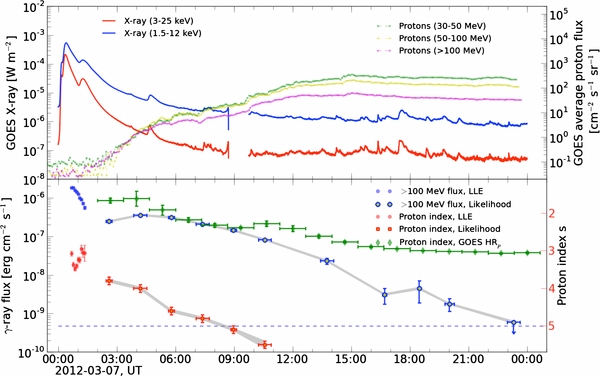
Figure 2. Long lasting emission. Top panel: soft X-rays (red: 1.5–12 keV, blue: 3–25 keV) from the GOES 15 satellite. On the right axis, five-minute averaged proton flux (green: 30–50 MeV, yellow: 50–100 MeV, magenta: >100 MeV). We display the average of detectors A and B. Bottom panel: high-energy gamma-ray flux above 100 MeV measured by the Fermi LAT. The blue/red circles represent the flux and the derived proton spectral index obtained with the LLE analysis (covering the initial period, when the instrumental performance was affected by pileup of hard-X-rays in the ACD tiles). The blue circles and red squares represent the flux and derived proton spectral index, respectively, obtained by standard likelihood analysis. Green diamonds are the GOES proton spectral indexes derived from the hardness ratio, as described in the text. The gray bands correspond to the systematic uncertainty associated with flux measurements and of the estimated proton index due to uncertainties on the effective area of the instrument. The horizontal dashed line corresponds to the value of the gamma-ray flux from the quiescent Sun, from Abdo et al. (2011).
Download figure:
Standard image High-resolution image3. FERMI GAMMA-RAY DATA AND ANALYSIS
Orbital sunrise for Fermi occurred less than six minutes after the peak of the first flare, triggering the GBM at 00:30:32.129 UT (causing the abrupt rate increase visible in Figure 1, middle panel). The second flare is also clearly visible in the BGO0 detector of the GBM.59 The Fermi LAT >100 MeV all sky count rate60 was dominated by the gamma-ray emission from the Sun,61 which was nearly 100 times brighter than the Vela pulsar in the same energy range. During the impulsive phase (the first 80 minutes) the X5.4 flare was so intense that the LAT ACD suffered from pulse pile-up (see the Appendix), so the standard IRFs could not be used. Instead, the spectral analysis that we performed for this time interval differs from that we made at later times; moreover, we exclude the impulsive phase from the localization analysis.
To limit the possible bias due to the so-called fisheye effect (events where the converted e+e− pair scatter toward the LAT z-axis are more likely to pass the event selection criteria than events that scatter away from the z-axis; Ackermann et al. 2012a, Section 6.4) we used the true position of the Sun when it was in the field of view of the LAT to calculate an energy and angle-dependent correction that was applied to the reconstructed photon direction on an event-by-event basis.
3.1. The Impulsive Phase
The first step in our analysis of the impulsive phase is to consider nine adjacent time intervals of LLE data (see the Appendix for a detailed description of the LLE technique). In particular, we included data for the region centered on the Sun at the time corresponding to the middle of each time interval and selected the intervals when the Sun was within 70° from the LAT boresight. For each time interval, we extract two sets of background LLE data at 30 orbits before and after the flare, when Fermi was at a similar geomagnetic location (see the Appendix for further information regarding this choice). At ±30 orbits (∼2 days) the location and attitude of the spacecraft are approximately the same as during the impulsive phase of the flare. The reconstructed direction in instrument coordinates is not the same after ±30 orbits; therefore we keep the reconstructed direction fixed and move the position of the region of interest (ROI), i.e., the region of the sky around the transient source that we are analyzing, in order to sample the same cosmic-ray-induced background rate as during the flaring episode. This last step is needed to average the two background data sets because the local cosmic-ray-induced background dominates the in-aperture celestial background. In this way we obtain nine source spectra and nine background spectra (one for each time interval during the impulsive phase analysis). We compute the LLE energy redistribution matrices for each of the nine intervals separately.
We fit the data between 100 MeV and 10 GeV using XSPEC62 to test three models. The first two are simple phenomenological functions that may describe bremsstrahlung emission from accelerated electrons, namely a pure power law (PL) and a power law with an exponential cutoff (PLEXP):
where Γ is the photon index and  co is the cutoff energy. We found that the data clearly diverge from a pure power-law spectrum and that the PLEXP provides a better fit in all time intervals considered. The third model uses templates based on a detailed study of the gamma rays produced from pion decay (updated from Murphy et al. 1987). In this model accelerated high-energy protons (and other ions) with an assumed energy distribution collide with particles of the solar atmosphere, creating π0 and π± mesons.63 A π0 quickly decays into two gamma rays, each having an energy of 67.5 MeV in the rest frame of the meson. The decay products of charged π± mesons (secondary e±) produce gamma rays via Bremsstrahlung or by annihilation-in-flight of the positrons, and microwaves via synchrotron radiation.64 The interactions between the accelerated and background protons (and ions) also produce nuclear de-excitation lines in the 1–10 MeV range, observable by the GBM. The analysis of the GBM observations of these flaring episodes will be presented in a subsequent paper.
The pion-decay templates used in our fits depend on the ambient density, composition and magnetic field, and on the accelerated-particle composition, pitch angle distribution and energy spectrum. The templates represent a particle population with an isotropic pitch angle distribution and a power-law energy spectrum (dN/dE∝E−s, with E the kinetic energy of the protons) interacting in a thick target with a coronal composition (Reames 1995) taking 4He/H = 0.1. To obtain the gamma-ray flux value we fit the data by varying the proton spectral index s from 2 to 6, in steps of 0.1. In this way, we fit the LAT data with a model with two free parameters, the normalization and the index, s. The time dependence of the >100 MeV gamma-ray flux and of the proton index, s, derived using LAT data, is displayed in the lower panel of Figure 1, and the numerical values are reported in Table 1, as well as the best fit parameters of the PLEXP model.
Table 1. Spectral Analysis of the Impulsive Phase
| Time Interval | Proton index | Fluxπa | Γ | co |
FluxPLEXPa |
|---|---|---|---|---|---|
| 2012/03/07 UT | MeV | ||||
| 00:38:52–00:43:52 | 3.07 ± 0.07 ± 0.09 | 21 ± 1 ± 4 | 0.07 ± 0.09 ± 0.2 | 130 ± 8 ± 10 | 18.0 ± 0.4 ± 4 |
| 00:43:52–00:48:52 | 3.36 ± 0.07 ± 0.1 | 18.7 ± 0.6 ± 4 | 0.26 ± 0.07 ± 0.1 | 107 ± 4 ± 10 | 16.3 ± 0.3 ± 4 |
| 00:48:52–00:53:52 | 3.48 ± 0.07 ± 0.1 | 15.5 ± 0.3 ± 3 | 0.23 ± 0.06 ± 0.1 | 106 ± 4 ± 10 | 14.1 ± 0.2 ± 3 |
| 00:53:52–00:58:52 | 3.40 ± 0.06 ± 0.1 | 14.4 ± 0.4 ± 3 | 0.19 ± 0.06 ± 0.1 | 109 ± 4 ± 10 | 12.7 ± 0.2 ± 3 |
| 00:58:52–01:03:52 | 3.23 ± 0.07 ± 0.1 | 12.7 ± 0.4 ± 3 | 0.18 ± 0.07 ± 0.1 | 114 ± 5 ± 10 | 10.9 ± 0.2 ± 2 |
| 01:03:52–01:08:52 | 3.25 ± 0.08 ± 0.1 | 9.6 ± 0.3 ± 2 | 0.25 ± 0.08 ± 0.1 | 111 ± 6 ± 10 | 8.6 ± 0.2 ± 2 |
| 01:08:52–01:13:52 | 2.95 ± 0.08 ± 0.09 | 9.0 ± 0.3 ± 2 | 0.00 ± 0.05 ± 0.1 | 136 ± 7 ± 10 | 7.2 ± 0.2 ± 2 |
| 01:13:52–01:18:52 | 3.0 ± 0.1 ± 0.09 | 7.2 ± 0.4 ± 1 | −0.6 ± 0.10 ± 0.1 | 220 ± 30 ± 20 | 6.0 ± 0.3 ± 1 |
| 01:18:52–01:23:52 | 3.1 ± 0.2 ± 0.1 | 5.7 ± 0.6 ± 1 | −0.8 ± 0.20 ± 0.1 | 270 ± 70 ± 30 | 5.0 ± 0.5 ± 1 |
Notes. In all cases the statistical errors are shown first and the systematic errors follow. aIntegrated energy flux between 100 MeV and 10 GeV, in units of 10−7 erg cm−2 s−1 and are calculated from the pion decay model (π) and for the exponential cut-off model (PLEXP).
Download table as: ASCIITypeset image
It appears that, after a short phase of spectral softening (00:40:00–00:53:00 UT), the proton spectral index hardens before and during the rising phase of the impulsive interval of the second flare (00:53:00–01:08:00 UT) as seen by the GBM detectors (middle panel of Figure 1). The spectral index s correlates better with the GBM flux than with the high-energy flux measured by the LAT. For interpretation of these results; see Section 4.
3.2. Temporally Extended Emission
We analyzed the data from after the first ninety minutes of Fermi-LAT observations using the standard likelihood analysis implemented in the Fermi-LAT ScienceTools65 with P7SOURCE_V6 IRFs, selecting gamma rays within an ROI of 12° radius centered on the sun and that arrived within 100° of the zenith to reduce contamination from the Earth's limb. We include the azimuthal dependence of the effective area in calculating exposures.
To study the temporally extended emission, we perform time-resolved spectral analysis in Sun-centered coordinates by transforming the reference system from celestial coordinates to ecliptic Sun-centered coordinates. This is necessary in order to compensate for the effect of the apparent motion of the Sun during the long duration of the flare. We select intervals when the Sun was in the FOV (angular distance from the LAT boresight <70°) and use the unbinned maximum likelihood algorithm gtlike. We include the isotropic template model that is used to describe the extragalactic gamma-ray emission and the residual cosmic ray (CR) contamination,66 leaving its normalization as the free parameter. Over short timescales, the diffuse Galactic emissions produced by CR interacting with the interstellar medium are not spatially resolved and are hence included in the isotropic template. We also add the gamma-ray emission from the quiescent Sun modeled as a point source located at the center of the disk, with a spectrum described by a simple power law with a spectral index of 2.11 and an integrated energy flux (>100 MeV) of 4.7 × 10⁻¹⁰ erg cm−2 s−1 (corresponding to a flux of 4.6 × 10⁻⁷ photons cm−2 s−1 as reported in Abdo et al. 2011). We did not include the extended Inverse Compton (IC) component described in Abdo et al. (2011) because it is too faint to be detected during these time intervals. We fit the data with the same two phenomenological functions used for the impulsive phase of the flare and use the likelihood ratio test to estimate whether the addition of the exponential cutoff is statistically significant. The test statistic (TS; Mattox et al. 1996) is defined as twice the increment of the logarithm of the likelihood  obtained by fitting the data with the source and background model components simultaneously. Because the null hypothesis (i.e., the model without an additional source) is the same for the two models, the increment of the TS (ΔTS = TSPLEXP-TSPL) is equivalent to the corresponding difference of maximum likelihoods computed between the two models.
For each interval, if ΔTS ⩾ 30 (roughly corresponding to 5σ) then the PLEXP model provides a significantly better fit than the simple power-law and we retain the additional spectral component. In these time intervals, we also used the pion decay model to fit the data and estimated the corresponding proton spectral index. We performed a series of fits with the pion decay template models calculated for a range of proton spectral indices. We then fit the resulting profile of the log-likelihood function with a parabola and determine its minimum ( ) and the corresponding value s0 as the maximum likelihood value of the proton index. The 68% confidence level is evaluated from the intersection of the profile with the horizontal line at −2
  (see insets in Figure 4). Table 2 summarizes our results.
Table 2. Spectral Analysis of the Time Extended Emission
| Interval | Start (UT) | Duration | TSPL | ΔTSa | Γ | co |
Fluxb | Proton Index | X,Y (r68⊕70)c |
|---|---|---|---|---|---|---|---|---|---|
| 2012/03/07 | s | MeV | arcsec | ||||||
| (a) | 02:27:00 | 1110 | 1336 | 85 | 1.0 ± 0.2 ± 0.05 | 250 ± 40 ± 4 | 2.4 ± 0.1 ± 0.2 | 3.8 ± 0.1 ± 0.1 | −280, 140 (320) |
| (b) | 03:52:00 | 2370 | 16318 | 987 | 0.9 ± 0.1 ± 0.04 | 210 ± 10 ± 2 | 3.55 ± 0.05 ± 0.3 | 4.0 ± 0.1 ± 0.1 | -450, 260 (100) |
| (c) | 05:38:32 | 1050 | 1393 | 159 | 0.2 ± 0.3 ± 0.04 | 120 ± 10 ± 2 | 3.1 ± 0.1 ± 0.2 | 4.6 ± 0.2 ± 0.1 | −470, 260 (350) |
| (d) | 07:03:00 | 2400 | 9003 | 756 | 0.4 ± 0.1 ± 0.03 | 130 ± 7 ± 1 | 2.07 ± 0.04 ± 0.2 | 4.8 ± 0.1 ± 0.1 | −500, 130 (150) |
| (e) | 08:50:00 | 1020 | 500 | 73 | −0.2 ± 0.6 ± 0.1 | 90 ± 20 ± 1 | 1.4 ± 0.1 ± 0.1 | 5.1 ± 0.3 ± 0.1 | 670, 580 (750) |
| (f) | 10:14:32 | 2370 | 1833 | 204 | −0.3 ± 0.2 ± 0.03 | 80 ± 9 ± 1 | 0.81 ± 0.03 ± 0.07 | 5.5 ± 0.2 ± 0.1 | 440, 380 (330) |
| (g) | 13:25:00 | 2400 | 137 | 13 | 2.9 ± 0.2 ± 0.02d | ⋅⋅⋅ | 0.23 ± 0.04 ± 0.02 | ⋅⋅⋅ | ⋅⋅⋅ |
| (h) | 16:36:00 | 780 | 17 | 8 | 2.9 ± 0.4 ± 0.02d | ⋅⋅⋅ | 0.03 ± 0.01 ± 0.003 | ⋅⋅⋅ | ⋅⋅⋅ |
| (i) | 18:24:00 | 540 | 10 | 3 | 3.7 ± 0.8 ± 0.03d | ⋅⋅⋅ | 0.04 ± 0.03 ± 0.004 | ⋅⋅⋅ | ⋅⋅⋅ |
| (j) | 19:47:00 | 1710 | 59 | 2 | 2.6 ± 0.3 ± 0.02d | ⋅⋅⋅ | 0.02 ± 0.01 ± 0.001 | ⋅⋅⋅ | ⋅⋅⋅ |
| (k) | 22:58:30 | 2370 | 7 | 4 | 1.6 ± 0.6 ± 0.01d | ⋅⋅⋅ | <0.006 | ⋅⋅⋅ | ⋅⋅⋅ |
Notes. In all cases the statistical errors are shown first and the systematic errors follow. aΔTS = TSPLEXP-TSPL. bEnergy Flux of gamma rays between 100 MeV and 10 GeV, in units of 10−7 erg cm−2 s−1, calculated using the best fit model. cA systematic error of 70 arcsec has been added in quadrature to the estimated 68% error radius, and is reported between parentheses. dThe value of the spectral index are obtained from the simple power-law fit.
Download table as: ASCIITypeset image
In Figure 3 we compare the observed count spectra with the predicted numbers of counts for the different models. The predicted numbers are the sum of the contribution of the background and of the flare, after the spectral parameters are optimized. The contribution of the isotropic background and of the quiescent Sun is also shown in the figures. In the first six time intervals (a through f) a power-law model does not correctly reproduce the data, while a curved spectrum (such as the power law with an exponential cut off or a pion decay model) provides a better description of the data. In the time intervals from g) to j) the power-law representation is adequate to describe the data; in the last bin, the flare is only marginally significant (TS = 7); the flux and the photon index are compatible with the values of the quiescent Sun. For this reason we have indicated the last point as an upper limit (computing the 95% C.L.). In the lower panel of Figure 2 we combine the LLE and likelihood analysis results, showing the evolution of both the gamma-ray flux and the derived spectral index of the protons.67 Unlike during the impulsive phase, the spectrum during the temporally extended phase becomes softer monotonically (s increases).
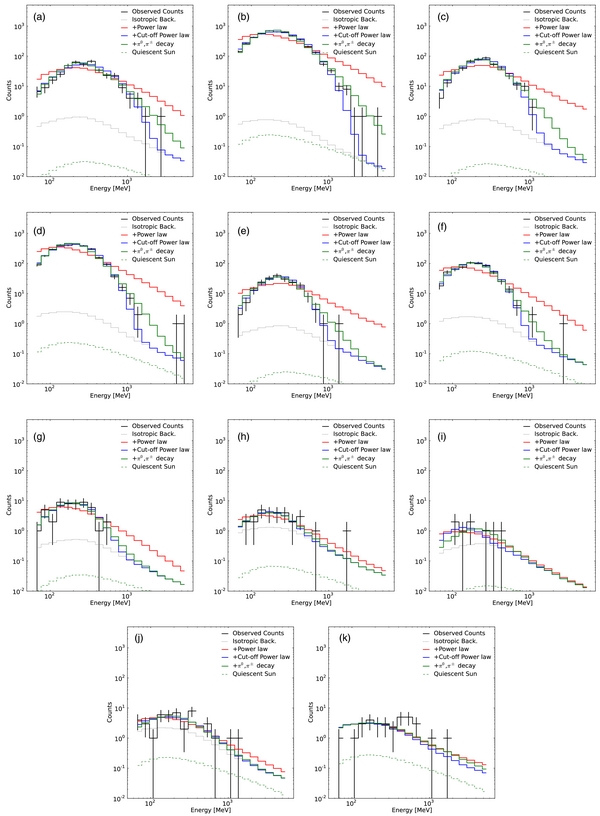
Figure 3. Comparison between observed counts (black thick line) and model predictions for the 11 time intervals defined in Table 2. The dotted black line is the isotropic background (sum of the Galactic and isotropic background) and the green dashed line is the contribution from the quiescent Sun. The red, green, and blue thick lines are the predicted numbers of counts from background + source modeling the solar flare with a PL, a PLEXP, and with a pion decay model, respectively. Statistical uncertainties are associated with the numbers of observed counts using the Gehrels (1986) prescription for confidence level in the low counts regime.
Download figure:
Standard image High-resolution imageWe also compare our results with the GOES proton spectral data. For this, we selected two energy bands (>30 MeV and >100 MeV) and corrected the light curve by the proton time-of-flight (TOF) to 1 AU by considering the TOF for 30 MeV and 100 MeV protons (i.e., the maximum delay in each energy band). As a measure of the spectral index of the SEP protons (sSEP), we compute the hardness ratio (HRp) defined as:
where P is the integral of the proton flux (assuming that the proton flux is proportional to a power law). The HRp is related to the value of the spectral index, sSEP, of the SEP protons observed at 1 AU, roughly as:

To estimate the uncertainty associated with this procedure we repeat the calculation neglecting the TOF correction. In this way we obtain two values for the SEP spectral index for each time bin, corresponding to the actual and zero delay due to the time of flight. In Figure 2 we report the estimated proton spectral index as the average of these two values and its uncertainty as half the difference of these two values. However, we note that the sSEP is for protons with energy less than a few hundred MeV while s is for protons with energies greater than 300 MeV. Diffusion is expected to play an important role in the transport of these SEPs but an in-depth transport analysis is beyond the scope of this paper. From our comparison we find that the proton spectral index inferred from the gamma-ray data is systematically softer than the value of the index derived directly from SEP observations but that the temporal evolution (hard-to-soft) is similar.
Uncertainties in the calibration of the LAT introduce systematic errors on the measurements. The uncertainty of the effective area is dominant, and for the P7SOURCE_V6 event class it is estimated to be ∼10% at 100 MeV, decreasing to ∼5% at 560 MeV, and increasing to ∼10% at 10 GeV and above. We studied the effect of the systematic uncertainties on our final results via the bracketing technique described in detail in Ackermann et al. (2012a). We find that the uncertainties on the flux are <10% and on the inferred proton index are <0.10. The results are represented by the gray bands in Figure 2 and in Table 2.
In the six time intervals where the ΔTS>30, we compute the photon spectral energy distribution. To do so we divide the data into 10 energy bins and determine the source flux using the unbinned maximum likelihood algorithm gtlike keeping the normalization of the background constant at the best fit value and assuming that the spectrum of the point source is an E−2 power law. Note that fixing the power law index provides one less degree of freedom and, with a the number of energy bins large enough (>4 per decade in energy), the results do not depend on the particular value chosen. For nondetections (TS < 9), we compute 95% CL upper limits. The results are shown in Figure 4. We also report the values of the energy flux in each energy bin for the six time intervals in Table 3.

Figure 4. Photon spectral energy distributions in the six time intervals in which the curved model provided a better fit ((a) through (f)). For each time interval we illustrate the models used for fitting the broadband spectrum: power law (dashed), power law with an exponential cutoff (dotted) and pion decay template model (solid). In the insets we report the profile of the likelihood function −2 which is used to estimate the pion template model that best matches the data. The scans are performed as functions of the index of the proton distribution used to compute the templates. The intersections with the horizontal dashed lines represent the 68% confidence levels used to estimate the errors.
Download figure:
Standard image High-resolution imageTable 3. Spectral Energy Distribution
| Energy Bin | Energy Flux | ||||||
|---|---|---|---|---|---|---|---|
| (MeV) | (× 10−9 erg cm−2 s−1) | ||||||
| (a) | (b) | (c) | (d) | (e) | (f) | ||
| 60–95 | 64 ± 17 | 117 ± 6 | 83 ± 21 | 79 ± 5 | 31 ± 14 | 40 ± 5 | |
| 95–150 | 79 ± 13 | 175 ± 6 | 171 ± 21 | 129 ± 5 | 96 ± 16 | 49 ± 4 | |
| 150–239 | 149 ± 14 | 211 ± 6 | 236 ± 19 | 134 ± 5 | 121.1 ± 14 | 65 ± 4 | |
| 239–378 | 137 ± 13 | 198 ± 6 | 190 ± 16 | 123 ± 5 | 76.2 ± 11 | 46 ± 4 | |
| 378–600 | 73 ± 10 | 123 ± 5 | 94 ± 12 | 56 ± 4 | 41.8 ± 8 | 16 ± 3 | |
| 600–950 | 49 ± 8 | 57 ± 4.2 | 36 ± 8 | 16 ± 2 | 7.5 ± 4 | <4 | |
| 952–1508 | 16 ± 6 | 19 ± 3 | <12 | 3 ± 1 | <12 | <2 | |
| 1509–2391 | <14 | 6 ± 2 | <10 | <2 | <10 | <4 | |
| 2391–3789 | <21 | <5 | <15 | <3 | <16 | <6 | |
| 3780–6000 | <22 | <5 | <25 | <7 | <26 | <8 | |
Note. The intervals (a)–(f) are those in which the ΔTS>30. See Table 2 for the start time and duration.
Download table as: ASCIITypeset image
3.3. Localizing the High Energy Gamma-rays
We measure the direction of the >100 MeV gamma-ray emission using the gtfindsrc tool and perform a likelihood analysis on both time-integrated and separate time intervals. The background is modeled using the best-fit parameters obtained by the time-resolved spectral analysis described in the previous section, and the source is modeled according to the best-fit model. The uncertainties on the localization are obtained by combining the 68% error radius from gtfindsrc with the systematic bias associated with the "fisheye" effect in quadrature. We estimate the latter using Monte Carlo simulations and find it to be 002 (≈70'').
The results for the six time bins where the ΔTS > 30 are shown in Figure 5. The coordinates of the centroids (with uncertainties) are shown in the last column of Table 2. For the remaining time intervals, the reconstructed location of the emission is consistent with the direction of the Sun, although the associated uncertainty is larger than the angular diameter of the Sun.
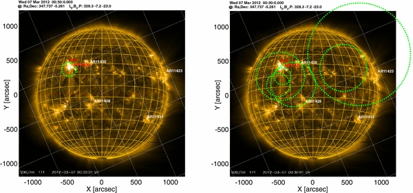
Figure 5. Location of the gamma-ray emission above 100 MeV for the time-integrated (left) and the time resolved (right) analyses. The background images are from SDO (AIA 171Å) and are taken at 00:30:00 UT on March 7. Active regions are flagged with their respective NOAA numbers. The region associated with the X-class flares is indicated with a red label, located at N16E30 (X,Y = −471,373''). The green circles are the 68% source location uncertainty regions (with systematic error added in quadrature). The grid on the background is the coordinate grid of equatorial coordinates, while the yellow sphere is the heliocentric coordinate grid (with the projected solar rotation axis parallel to the Y-axis; the Z-axis is the line of sight (from the Sun to the observer) and the X-axis in the Cartesian projection completes the normal basis.
Download figure:
Standard image High-resolution imageDuring the ∼20 hr of detected flaring gamma-ray emission, the LAT measured five photons with E > 2.5 GeV and reconstructed direction less than 1° from the center of the solar disk. Given the importance of these high-energy events and the variation of the PSF across the wide field of view (2.4 sr) of the LAT, we further investigate the characteristics of these photons. All five of these events belong to the P7SOURCE_V6 event class and three of them are also P7ULTRACLEAN_V6 (see Abdo et al. 2009b for a detailed description of the photon classes). Two of these photons, with energies 2.8 GeV and 4 GeV, were detected during the impulsive phase of the flare and the remaining three during the extended emission, including one with 4.5 GeV energy at 07:30:00 UT. Comparing the distance from the center of the solar disk and the predicted 68% containment radius from the point-spread function (PSF) of the instrument we find that four of the events are consistent with the solar disk. In the case of the 4.5 GeV photon, the reconstructed direction is 08 from the center of the solar disk and the 68% containment radius is approximately 02. Therefore, we conclude that the reconstructed direction of this event is only marginally consistent with the solar disk.
Considering the average rate of LAT-detected photons above ∼2.5 GeV coming from an ROI with radius 1° centered at the Sun (calculated using all available flight data, excluding the bright LAT-detected solar flare time intervals) we find that the probability to observe five or more events in 8 hr due to Poisson fluctuations is approximately P = 8.0 × 10⁻⁶ (∼4.8σ). In Table 4 we list some of the basic properties of these photons.
Table 4. High Energy Gamma Rays from the Solar Flare
| Arrival Time | Energya | Distanceb | θc | Event Class | PSF |
|---|---|---|---|---|---|
| 2012/03/07 UT | (GeV) | (°) | (°) | (°) | |
| 0:49:37.8 | 2.8 | 0.2 | 49 | SOURCE | 0.3 |
| 1:18:44.6 | 4.0 | 0.6 | 66 | ULTRACLEAN | 0.5 |
| 2:35:01.7 | 2.9 | 0.6 | 62 | SOURCE | 0.6 |
| 4:12:28.4 | 2.9 | 0.5 | 36 | ULTRACLEAN | 0.6 |
| 7:30:24.6 | 4.5 | 0.8 | 44 | ULTRACLEAN | 0.2 |
Notes.
aThe energy resolution at 3 GeV and 50° off-axis angle is of the order of 7%.
bReconstructed distance from the center of the solar disk.
cReconstructed direction with respect to the instrument coordinate system.
dPSF corresponds to the 68% containment radius calculated from the PSF of the instrument for the energy and direction of the gamma ray.
Download table as: ASCIITypeset image
4. DISCUSSION AND INTERPRETATION
The Fermi-LAT observations of the two exceptionally bright flares of 2012 March 7 provide an excellent opportunity to study the spectral evolution of the gamma-ray emission during the impulsive phase and throughout the temporally extended phase. Furthermore, due to the high sensitivity of the LAT we can localize the >100 MeV emission originating from the solar flare, which provides new information that can be used to constrain the emission and acceleration processes as described below.
As seen in Figure 1, GOES fluxes began to rise at about 00:02:00 UT, and continued to increase for over an hour, while Fermi sunrise started at 00:30:00 UT, roughly six minutes after the peak of the first X5.4 flare. This coincided with the gradual decay phase during which the hard X-ray (HXR) emission observed with GBM is relatively soft. The GBM detected only weak emission above 100 keV during this phase of the first flare. During the second X1.3 flare GBM detected a large flux in the 100–300 keV range and a significant flux above 1 MeV which indicates acceleration of electrons or protons up to several MeV. The derivative of the GOES flux shows a pulse shape similar to that of the lowest energy GBM channel. These pulses show the usual soft–hard–soft spectral evolution (see, e.g., Hudson & Fárník 2002) in the HXR regime.
The LAT >100 MeV emission decreases monotonically (approximately with an exponential decay time of ∼30 minutes) with no significant evidence for an upturn during the second flare. However, the derived proton spectral index s, obtained from the pion-decay model, shows some variation ranging between ∼3.0 and ∼3.5. The spectrum is initially soft, but then exhibits evidence of spectral hardening during the second flare, which is also the case in the HXR regime (Figure 1). The hardening of the LAT spectrum seems to start ∼20 minutes before the start of the X1.3 flare. However, the significance of this early hardening is less than 3σ. Such a spectral hardening during the decay phase can either be due to an intensification of the acceleration rate or trapping of accelerated particles in a coronal loop (see discussion below).
The temporally extended emission is characterized by a slight increase of the gamma-ray flux starting at approximately 2:15:00 UT; the flux reaches its maximum at approximately 4:00:00 UT. The peak of the light curve is broad and the flux after t0 = 12:00:00 UT decays exponentially as F(t)∝exp [ − (t − t0)/τ], with τ ≈ 2.7 hr. The gamma-ray spectrum and thus the required particle spectrum softens monotonically during the first six time intervals, with no sign of an early rise or a plateau as seen in the flux. The hardness ratio of the SEP protons also shows similar softening except some deviation is apparent at about 10:00:00 UT which could be due to the subsequent GOES event at 05:00:00 UT. The SEP proton spectrum in the 30–100 MeV range is harder (index smaller by 2–3 units) than the spectrum of the >300 MeV protons required for production of the gamma rays (see bottom panel of Figure 2).
We now describe to what extent these new observations constrain the models. In particular, we discuss continuous versus prompt acceleration in a magnetic trap, proton versus electron emission, and acceleration at the coronal reconnection site versus CME shock.
4.1. Prompt versus Continuous Acceleration
In the prompt acceleration model particles are injected quickly, e.g., as a power-law spectrum, into a trap region where they gradually lose energy and emit radiation (Murphy et al. 1987; Kanbach et al. 1993). If the radiation is produced in the trap region then we expect a spectral variation that depends on the energy dependence of the energy loss rate (Aschwanden 2004). For relativistic electrons the energy loss rate due to Coulomb collisions and synchrotron emission is given by
where δ = 2 and for flare conditions τ0 ∼ 104 s (1010 cm−3n−1) and Ep ∼ 10 MeV (n/1010 cm−3)1/2(100 G/Beff). This produces characteristic spectra that become flat at low energies, E < Ep due to Coulomb energy losses, and develop a sharp cut off at high energies, E > Ep due to synchrotron and IC losses, in less than an hour (see, e.g., Petrosian 2001).68 This clearly disagrees with the data that indicate a power-law spectrum at low energies with a gradual high-energy cutoff. A similar expression with δ = 1, Ep ∼ 10 GeV and τ0 ∼ 3 s (1010 cm−3n−1) day applies for 0.1–100 GeV protons with high-energy losses due to inelastic p–p interactions. This will cause some initial hardening of the spectra (index decreasing by ∼1) at low energies within several hours, and the higher-energy emission should persist for several days, which also disagrees with the observed spectral evolution. The marginally significant hardening within a few minutes before the X1.5 flare requires a density of n ≫ 1010 cm−3, which is not appropriate for a coronal trap model (Ryan 1986).
An alternative scenario is the trap precipitation model (Bai 1982) where the particles trapped in a magnetic bottle (converging field lines) are scattered into the loss cone that causes their precipitation into the chromosphere and below, where they lose most of their energy and produce gamma rays. Coulomb collisions cannot be the agent for this scattering, because the relativistic electron Coulomb scattering rate is lower than the Coulomb energy loss rate by a factor of γ2 (where γ = E/mec2) and is much smaller than synchrotron energy loss or IC scattering rate (see, e.g., Table 1, Petrosian 1985). The Coulomb scattering rate for protons is lower than their energy loss rate by a factor proportional to the electron to proton mass ratio. In other words, with Coulomb scattering the particles lose energy before they are scattered into the loss cone. Therefore, a much faster scattering rate is required for this scenario. Scattering by turbulence could be a possibility but (1) in that case acceleration by turbulence will also be present so we no longer have a prompt model, and (2) gradual softening of the spectra will require a higher rate of scattering into the loss cone for higher energy particles, which may require a turbulence spectrum much steeper than Kolmogorov (see, e.g., Pryadko & Petrosian 1997). Thus, we conclude that trapping is negligible and relativistic electrons and protons of all energies are transported to the chromosphere and below within the transport time L/v ∼ 0.1 s (for L ∼ 109 cm) where they lose energy rapidly and emit radiation as in the standard thick target model discussed below. Therefore, a more likely scenario is continuous acceleration (e.g., by turbulence; see Petrosian & Liu 2004) with a timescale comparable to, or shorter than, the particle energy-loss timescale. Continuous acceleration, as first proposed by Ryan & Lee (1991), was also favored to explain the COMPTEL observations (Rank et al. 2001) of extended emission in the solar flares of 1991 June. Observations of 2.223 MeV neutron capture radiation indicate continuous acceleration of ions, lasting for as long as several hours in the 1991 June 11 solar flare.
4.2. Electron versus Proton Emission
For electrons, nonthermal bremsstrahlung is the only viable mechanism of gamma-ray production (Trottet & Vilmer 1984; Vilmer 1987) and requires >100 MeV electrons. However, the very hard (flat) observed photon spectra with low-energy power-law indices (Γ < 1) require a very hard injected electron spectrum. In the thick target model and for relativistic electrons this means δinj ∼ Γ + 1 < 2. This is much harder than spectra deduced from hard X-ray impulsive phase emission in most flares. However, as shown by Park et al. (1997), at high energies bremsstrahlung spectra can deviate significantly from a power law and have a rollover as observed here. However, a spectral rollover at >100 MeV requires a weaker magnetic field than those expected in the corona.
In the corona the energy loss rate of >100 MeV, electrons are dominated by synchrotron losses with a timescale of τsync ∼ 30 (GeV/E)(100G/B)2 s. The IC loss time is longer τIC ∼ 6 × 10³(GeV/E) s and the bremsstrahlung time, though shorter than Coulomb losses, is even longer: τbrem ∼ 3 × 10⁴(1010 cm−3/n)(GeV/E)0.1 s. However, all these times are longer than the transport time so that electrons lose a small fraction of their energy in the corona above the transition region. If the magnetic field reaches 103 G synchrotron losses can become important with roughly a few percent of electron energy going into production of 1.5–150 THz radiation. Below the transition region density increases rapidly (within few hundred kilometers) and electrons are stopped at a column depth of ∼1025 cm−2 or density of ∼1017 cm−3, where they lose most of their energy producing bremsstrahlung radiation in a very short (0.01 s) time (see Petrosian et al. 1994), but with a total loss time of ∼L/v ∼ 0.1 s. This short time and the hard spectrum requires a very efficient acceleration which may be problematical considering the fact that the highest-energy photon observed by the Fermi-LAT of 4 GeV would require electrons to be accelerated to about 10 GeV. The above conclusion involved some assumptions and depends on the values of some critical parameters like the height of the accelerator and magnetic field. For a higher source or larger magnetic field, the acceleration time can be shorter and fraction of energy lost via synchrotron and bremsstrahlung processes will be different. Clearly, this requires a more detailed treatment of acceleration, transport, and emission processes, which is beyond the scope of this paper.
The situation is very similar and somewhat simpler for protons because protons with E < 1 GeV lose energy primarily via Coulomb collisions with background electrons with a loss time τL ∼ 3 × 10⁴(1010 cm−3/n)(E/GeV) s and through pion production in collisions with background protons at higher energies with a loss time of τL ∼ 3 × 10⁵(GeV/E)0.1 s at E > 10 GeV. Again these times are much longer than the transport time to the transition region (up to the acceleration height of L < 1014 cm) so that most of the energy loss and radiation takes place below the transition region. For example, 300 MeV protons penetrate to column depths and densities very similar to those given above for electrons and lose energy in much less than a second. Thus, the situation is very similar to that of electrons except that the energy dependence of the proton loss rate varies in the range of proton energies of interest and the effective thick target spectrum Neff(E) of protons per energy unit E for a continuous injection spectrum  is given by
so that for an injected power-law  the effective spectrum will be a broken power-law steepening with an index change of about one around several GeV. Whether such a spectrum can describe the observations adequately is beyond the scope of the current paper. It should also be noted that the yield of gamma rays is about 1% at the pion production threshold of ∼300 MeV but becomes essentially 50% above a few GeV (the other half of the proton energy going to neutrinos).
In summary, both relativistic bremsstrahlung emission by electrons or decay of pions produced by >300 MeV protons describe the observations in a thick target model with acceleration time shorter than the transport time from the acceleration site to the thick target below the transition region. However, an unusually hard spectrum of electrons is needed while the required proton spectra are similar to those derived from other observations. Thus, pion decay seems to be the preferred radiation mechanism, in accord with conclusions reached by Rank et al. (2001) for the 1991 June flares mentioned above, based on the COMPTEL detection of the 2.2 MeV neutron capture line.
From the results of the gamma-ray spectral analysis in the proton scenario, and using the gamma-ray yield, we estimate the number and energy of the accelerated protons with kinetic energy >30 MeV producing gamma rays and compare with the observed SEPs. During the first impulsive phase the estimated number (energy) of protons interacting with the Sun is Np ∼ 2.5 ×1033 ( 2.2 × 1029 erg), while for the temporally extended emission, these are approximately Np ∼ 1.0 × 1034 (
 7.2 × 1029 erg).
From the GOES observations, we can roughly estimate the number (energy) of SEP protons escaping the CME shock. We integrate the flux observed by GOES detectors, assuming isotropic emission, and that the CME leading edge propagated toward the Earth with an almost-constant speed of ≈2600 km s−1 until 20 R☉. We do not have accurate measurements of the speed of the CME after this distance, so we use the information that it reached the Earth at approximately 10:42 UT of March 8 assuming constant acceleration (−0.02 km s−2). We calculate the position of the CME leading edge and we calculate the number of protons during the period of time when the gamma-ray flux was high (until approximately 23:00:00 UT on March 7); we obtain: NSEP ∼ 3 × 1033 ( 1.0 × 1030 erg).69 A more detailed calculation of the flux of accelerated particles at the CME shock, properly considering propagation affects and non-isotropic emission, is beyond the scope of this paper, but considering that this is only a fraction (<20%) of the SEP measured (i.e., the proton flux measured by GOES remains high until approximately 20:00:00 UT of March 12), we conclude that protons producing gamma rays carry significantly less energy than SEP protons observed by GOES.
4.3. Acceleration at the Corona versus CME Shock
Continuous acceleration of protons at the flare reconnection region, whether by a stochastic acceleration mechanism (Petrosian & Liu 2004) or by commonly postulated standing shock (see, e.g., Aschwanden 2004; Mann et al. 2006) can account for most of the spectral observations described above. In this model protons escape the acceleration site along closed field lines into the chromosphere and the spectral changes are simply due to the softening of the spectrum of protons as the flare decays. As shown by Petrosian & Liu (2004), in stochastic acceleration by turbulence (or by a standing coronal shock; see Petrosian 2012) the accelerated particle spectra become softer (harder) as the turbulence becomes weaker (stronger), which can naturally explain the observed spectral evolution both in the prompt and extended emission phases. Acceleration at the CME shock (Rank et al. 2001) is also an attractive possibility because the Large Angle and Spectrometric Chronograph (LASCO; Brueckner et al. 1995) on board the Solar and Heliospheric Observatory (SOHO) mission observed a fast CME ejected at approximately 00:30:00 UT, and measured the speed of the head of the fastest segment of the leading edge (Gopalswamy et al. 2009) to be 2684 km s−1. The shock front of a CME is known to accelerate SEPs, sometimes to energies >300 MeV required for gamma-ray production Reames (2013), but its contribution to the acceleration of the particles that produce gamma rays remains unclear. The SEP protons observed by GOES are those accelerated by the shock and escape from the upstream region of the shock (see, e.g., Ramaty et al. 1990). There are also indications that a reservoir of accelerated particles exists in the downstream region of the shock behind the CME Reames (2012, 2013); Zank et al. (2000). However, as mentioned above, gamma-ray production would be too weak to be detected by Fermi-LAT, because of prevailing low densities (≪1010 cm−3). The accelerated particles must be transported to higher densities below the corona for efficient production of radiation. This requires existence of field lines connecting the reservoir to the Sun. We estimate that in 10 hr the CME would have traveled approximately 80 R☉(∼0.4 A.U.). Whether such a connection can be maintained over this distance is matter of speculation. It is possible that the outflow results in a current sheet behind the CME that can provide a magnetically connecting path to the original flare site. The displacement of the reconstructed LAT emission centroid at later times can be explained by a larger dispersion of particles due to the longer distance traveled. This model provides the correct scenario for short acceleration time scales (∼1 hr).
The second difficulty is that the SEP spectra are much harder than the proton spectra deduced for the extended emission phase but their spectral index is similar to the impulsive phase index of the protons. It is not clear why the upstream and downstream protons would have such different spectra. One possible scenario is that during the extended phase protons are accelerated in the corona while the SEP protons are a result of the re-accelerated of prompt phase protons at the CME shock.
In summary, in this paper we have presented an analysis of the brightest solar flare detected by the Fermi LAT to date. We have shown that during most of the long-duration emission the gamma rays appear to come from the same active regions responsible for the flare emission. The fluxes and spectra of the high-energy gamma rays evolve differently during the impulsive phase and the sustained emission. Also there are correlations and some differences between the fluxes and spectral indexes of the protons required for the production of high-energy gamma-rays and SEP protons seen at 1 AU. From these results we suggest that the high-energy gamma rays are most likely produced by protons (rather than electrons) accelerated in the corona (rather than in the associated fast CME shock) continuously during the entire flare.
The Fermi LAT Collaboration acknowledges generous ongoing support from a number of agencies and institutes that have supported both the development and the operation of the LAT as well as scientific data analysis. These include the National Aeronautics and Space Administration and the Department of Energy in the United States, the Commissariat à l'Energie Atomique and the Centre National de la Recherche Scientifique/ Institut National de Physique Nucléaire et de Physique des Particules in France, the Agenzia Spaziale Italiana and the Istituto Nazionale di Fisica Nucleare in Italy, the Ministry of Education, Culture, Sports, Science and Technology (MEXT), High Energy Accelerator Research Organization (KEK) and Japan Aerospace Exploration Agency (JAXA) in Japan, and the K. A. Wallenberg Foundation, the Swedish Research Council and the Swedish National Space Board in Sweden.
Additional support for science analysis during the operations phase is gratefully acknowledged from the Istituto Nazionale di Astrofisica in Italy and the Centre National d'Études Spatiales in France. We also wish to acknowledge G. Share for his continuous support and important contribution to the Fermi LAT collaboration and the anonymous journal referee for the useful comments and suggestions.
APPENDIX: THE LAT LOW ENERGY ANALYSIS
The LAT Low energy (LLE) technique is an analysis method designed to study bright transient phenomena, such as GRBs and solar flares, in the 30 MeV–1 GeV energy range. The LAT collaboration (Atwood et al. 2009) developed this analysis using a different approach than the one used in the standard photon analysis which is based on sophisticated classification procedures (a detailed description of the standard analysis can be found in Atwood et al. 2009; Ackermann et al. 2012a). The idea behind LLE is to maximize the effective area below ∼1 GeV by relaxing the standard analysis requirement on background rejection. The basic LLE selection is based on a few simple requirements on the event topology in the three sub-detectors of the LAT namely: a tracker/converter (TKR) composed of 18 x–y silicon strip detector planes interleaved with tungsten foils; an 8.6 radiation length imaging calorimeter (CAL) made with CsI(Tl) scintillation crystals; and an ACD composed of 89 plastic scintillator tiles that surrounds the TKR and serves to reject the cosmic-ray background.
First of all, an event passing the LLE selection must have at least one reconstructed track in the TKR and therefore an estimate of the direction of the incoming photon. Secondly, we require that the reconstructed energy of the event be nonzero. The trigger and data acquisition system of the LAT is programmed to select the most likely gamma-ray candidate events to telemeter to the ground. The on board trigger collects information from all three subsystems and, if certain conditions are satisfied, the entire LAT is read out and the event is sent to the ground. We use the information provided by the on board trigger in LLE to efficiently select events which are gamma-ray like. In order to reduce the amount of photons originating from the Earth limb in our LLE sample we also include a cut on the reconstructed event zenith angle (i.e., angle <90°). Finally, we explicitly include in the selection a cut on the ROI, i.e., the position in the sky of the transient source we are observing. In other words, the localization of the source is embedded in the event selection and therefore for a given analysis the LLE data are tailored to a particular location in the sky.
A.1. LLE Response Files
The LLE response files are generated based on dedicated Monte Carlo simulations. The simulations are used to study how the detector is "illuminated" by a source of a known flux and known position, during the real pointing history of the LAT. We do this by simulating a bright point source with a spectrum dN/dE ∼ E−1 at the position of the source in question (the Sun in this case), and using the pointing information saved in the spacecraft data file (FT2 file). We use the Fermi-LAT full simulator (Baldini et al. 2006) to generate particles from the point source, incident over a cross-sectional area of 6 m2, which illuminates the entire LAT. The LAT detector is represented by a complex model containing more than 34000 volumes. Gamma-ray conversion and particle propagation through the detector is implemented using GEANT4 (Geant4 Collaboration et al. 2003) while digitization and reconstruction are done using the same algorithm used for flight data. We then apply the LLE selection and bin the resulting events in reconstructed energy versus Monte Carlo energy (McEnergy) obtaining the so-called Redistribution Matrix, Rij. This matrix is proportional to the probability that an incoming photon of energy E ∈ [Ej, Ej + 1] will be detected in the reconstructed energy bin [Ei, Ei + 1]. We re-normalize each bin such that:
where NTOT is the total number of simulated events over an area of 6 m2 (typically 107), Nj is the number of detected events (that survive the selection cuts) with a McEnergy between Ej and Ej + 1. Aj is usually defined as the effective collecting area of the instrument. The Redistribution Matrix File (RMF) is saved in the standard HEASARC RMF File Format.70
A.2. Orbital Background Subtraction
In the case of short and bright transient gamma-ray sources, it is possible to select time windows before and after the transients (the "off-pulse" region) and, excluding the time window of the transient itself, fit the count rates in the off-pulse region with a polynomial function and in this way estimate, the background in the time interval of the transient. For LLE data, this analysis is described in Pelassa et al. (2010) and was applied to the 2010 June 12 flare, as presented in Ackermann et al. (2012b). This approach relies on a few assumptions: the background should not vary too much during the transient emission and also the amount of statistics should be sufficient to constrain the fit. These assumptions usually are satisfied when the interval of the transient emission is shorter than the Fermi orbital period (≈90 minutes).
For the 2012 March 7 flare presented here, the standard LLE approach to estimate the background by fitting the intervals before and after the flare could not be used because the flaring episode lasted longer than the orbital period. Instead, we estimate the background using data acquired in other orbits. Fermi passes through approximately the same geomagnetic configuration every 15 orbits, but given the standard rocking profile (alternating one orbit north and one orbit south) only the 30th orbit approximates similar geomagnetic and pointing conditions, and consequently a similar background rate. We do not average multiples of 30 orbits because they become less reliable, as they span observations further removed in time. This method of background estimation has been used for a number of background-dominated instruments in solar flare analyses, including historically for SMM-GRS (Vestrand et al. 1987; Murphy et al. 1990) and EGRET Kanbach et al. (1993)71 and currently for Fermi GBM (Fitzpatrick et al. 2011).
The background files produced for each interval are saved as standard PHA-I72 files. We used XSPEC to execute a forward-folding fit, where the model M(p1, p2, ...) is folded with the redistribution matrix, Rij, and the results are compared with the background-subtracted signal Si:
where Mj(p1, p2, ...) is the expected number of events between Ej and Ej + 1 for the time interval being analyzed. A maximum likelihood algorithm is then used to calculate the set of parameters that best model the data (see the XSPEC manual for details.)
A.3. Validation and Systematic Uncertainties
A detailed paper on the assessment of the systematic errors is in preparation; here we summarize the main results. Generally speaking, discrepancies between the actual response of the LAT and the response matrix derived from simulations can cause systematic errors in spectral fitting. We investigated the systematic uncertainties tied to the LLE selection by following the procedure described in Abdo et al. (2009b). In particular, we compared Monte Carlo with flight data, using the Vela pulsar (PSR J0835–4510) as a calibration source. The pulsed nature of the gamma-ray emission from this source (Thompson et al. 1975) gives us an independent control on the residual charged particle background. In fact, off-pulse gamma-ray emission is almost entirely absent, and a sample of "pure photons" can be simply extracted from the on-pulse region, after the off-pulse background is subtracted. Considering all time intervals during which the Vela pulsar was observed at an incidence angle θ < 80°, we estimate the discrepancy between the efficiency of the LLE selection criteria in the LAT data and in Monte Carlo to be ∼17% below 100 MeV, decreasing down ∼8% at higher energies, with an average value ∼9% (note that this average is weighted by the Vela spectrum).
Additionally, we performed a spectral analysis of the Vela pulsar, comparing LLE results with standard likelihood analysis. The >100 MeV flux obtained from the LLE analysis is 20% lower than published in Abdo et al. (2009a) and 16% less than the flux reported by Abdo et al. (2010). This discrepancy can be attributed to the fact that the selection criteria between LLE and the standard LAT likelihood analysis are rather different with the later being much looser. Whereas the differences found between the >100 MeV flux obtained from the LLE analysis and those published in Abdo et al. (2009a, 2010) are because our knowledge of the LAT performance improved with time and thus the value of the systematic uncertainties decreased. In our analysis of the impulsive phase of the 2012 March 7, we take this discrepancy into account by modifying the redistribution matrix Rij in order to reproduce the discrepancy observed on the Vela spectrum. To do this, we scale the redistribution matrix by a conservative ±20% and also we apply a scaling function as a function of the energy, going from ±10% below 250 MeV to ±10% above 250 MeV. These functions maximize the impact of the systematic uncertainty on the value of the measured flux and spectral index, and, at the same time, provide results that are compatible with the observed discrepancy of the Vela spectrum. We use the modified redistribution matrices to repeat the analysis, ousting bracketing value for the flux and the derived proton indexes. These are represented by the grey bands in Figure 1. Note that systematic uncertainties related to the LLE analysis are slightly larger than the ones related to the standard likelihood analysis due to the fact that LLE extends the analysis at lower energy where the value of the uncertainties are typically larger.
Finally, we also studied the energy resolution using large samples of simulated events with the Fermi-LAT full simulator. No significant bias was found, and the energy resolution for LLE is estimated to be ∼40% at 30 MeV, ∼30% at 100 MeV and <15% for energies greater than 100 MeV.
A.4. File Format and Availability
LLE data are generated for each burst (GRB or solar flare) that trigger the GBM. We first bin the data in energy and time, and, following the procedure described in Ackermann et al. (2013), we select the background region by selecting all the LLE events before the trigger and after 300 s from the trigger. We fit each energy bin with a polynomial function of the cosine of the source bore-sight angle as a function of time and we interpolate the background fit into the signal region. We evaluate statistical fluctuation of the signal above the expected background. This procedure is optimized taking into account different signal region and different time binning. We finally look at the post trial probability. Every detected signal with a post trial probability greater than 4σ is promptly made available through the HEASARC Web site.73 For each such detected GRB or solar flare, six different files are delivered.
- 1.The LLE event file format is similar to the LAT photon file format with some exceptions. Because the LLE data are tightly connected to a particular object (position and time), the FITS keyword OBJECT has been added to the file. Generally, OBJECT will correspond to the entry of the GBM Trigger Catalog74 used to generate LLE data and corresponds to the "name" column in the FERMILLE table (and in the GBM Trigger Catalog table). The direction of the source used for selecting the data for the LLE file is also written in the header of each extension of each LLE file. PROC_VER corresponds to the iteration of the analysis of LLE data. PASS_VER corresponds to the iteration for the reconstruction and the general event classification (Pass6, Pass7, etc.). VERSION corresponds to the version of the LLE product for the particular GRB or solar flare represented in the file.
- 2.The CSPEC file is obtained from directly binning the LLE event files. It provides a series of spectra, accumulated with 1 s binning (typically from −1000 to 1000 s around the burst). Each spectrum is binned in 50 energy channels, ranging typically from 10 MeV to 100 GeV. The format of the CSPEC file is tailored to satisfy rmfit75 standards, and it is not directly usable in XSPEC.
- 3.The CSPEC Response file (the RSP file) is the detector response matrix calculated from Monte Carlo simulation, and it corresponds to a single response matrix for each GRB or solar flare.
- 4.The PHA-I file contains the count spectrum. The PHA-I file is created from the same time interval used to compute the response matrix.
- 5.The selected events file is identical to the LLE event file with an additional selection on time interval applied to match the selection used to compute the response matrix and PHA-I files.
- 6.The LAT pointing and livetime history file is identical to the standard LAT file but with entries every s (instead of every 30 s). It typically spans the range ±4600 s from the trigger time.
The complete LLE selection used to select the events is saved in the keyword LLECUT in the primary header of each LLE file. If the GBM catalog position of the burst is updated (due to a refined localization from the LAT or Swift or from subsequent on-ground analysis), the LLE data are automatically updated and new versions of the LLE files are produced. In some cases, LLE data are manually generated (using a better localization which may or may not have been used in the GBM Trigger Catalog). If the direction of a GRB is revised based on follow-up observations with other instruments, regenerated LLE files will have the VERSION number incremented, but will leave the PASS_VER and PROC_VER unchanged.
In general we do not deliver the background estimates for the time ranges around the burst triggers, and we let the user estimate the background using the procedure described in Pelassa et al. (2010). For the reason explained above, we cannot perform this analysis on the 2012 March 7 flare. Therefore, for this particular flare, we provided LLE data including background files.
Footnotes
- 58
- 59
We use dead-time corrected count rates from the NaI2 in the 10–25 keV and 100–300 keV energy bands and from the BGO0 in the 1–10 MeV energy band. Subscripts refer to GBM NaI and BGO detector numbers.
- 60
This is for P7SOURCE_V6 class with gamma-ray zenith angles limited to zmax = 100°.
- 61
Illustrated by the Astronomy Picture of the Day, http://apod.nasa.gov/apod/ap120315.html.
- 62
- 63
The threshold energy for pion production by proton reactions is ∼300 MeV and ∼200 MeV/nucleon for alpha reactions.
- 64
Inverse Compton scattering of solar optical photons (
∼ 1 eV) by ∼50 MeV e± will produce hard X-ray photons of energy ∼20 keV. - 65
We used ScienceTools version 09-28-00 available from the Fermi Science Support Center http://fermi.gsfc.nasa.gov/ssc/.
- 66
We used iso_p7v6source.txt available from the Fermi Science Support Center.
- 67
After approximately 11:00:00 UTC the flux of the Sun diminished to the point that the spectral index of the proton distribution cannot be significantly constrained.
- 68
Because of IC loss by optical photons of energy density uph we have
 and even for B = 0, in the optical photon field of the Sun Beff ∼ 10 G and the energy loss timescale is less than one day.
 - 69
The relative values for protons at other energies will differ from the above numbers because of the differences in flare and SEP indices.
- 70
- 71
In Kanbach et al. (1993) an average for ± N × 16 orbits (for N = 1, 2, 3) was used.
- 72
- 73
- 74
- 75