COLLECTIVE PROPERTIES OF NEUTRON-STAR X-RAY BINARY POPULATIONS OF GALAXIES. II. PRE-LOW-MASS X-RAY BINARY PROPERTIES, FORMATION RATES, AND CONSTRAINTS

The conditions required for the formation of a CE have been much studied in the literature (for detailed reviews, see, e.g., Taam & Sandquist 2000; Webbink 2008). The essential ingredients for viable formation of a CE are (1) an extreme mass ratio and (2) an evolved primary. Depending on the evolutionary stage of the primary, three regimes of the primary's Roche-lobe overflow, namely, Cases A, B, and C, have been defined and are widely used in the literature. The cases of interest to us here usually belong to Cases B and C, involving an evolved primary. (Case A occurs when the donor is on main sequence, which can happen in very close primordial binaries, but this case is not of interest here, since it would lead to a merger during spiral-in, as explained earlier). The other condition, i.e., that of extreme mass ratio, is usually taken as q < 0.3 (van den Heuvel 1991, 1992), because in this regime the thermal timescales of the two stars are different by an order of magnitude or more. This regime of q-values is completely disjoint from that relevant for the HMXB progenitors (see Paper I), as expected. The mass of the secondary remains unchanged during the entire evolution from primordial binary to Roch-lobe overflow, as explained earlier. The upper limit to this mass is usually taken as 1–2 M_☉, although some authors have suggested somewhat higher limits (Podsiadlowski et al. 2002; Pfahl et al. 2003), in which case there is expected to be considerable mass loss in the initial phases of LMXB operation. For typical primary masses in primordial binaries, which are in the range 9–30 M_☉ for LMXBs, the mass ratio q thus always satisfies the above criterion of extremeness.

Quantitative descriptions of the binary-parameter changes in the CE phase can be given from the general picture of CE evolution given above (Webbink 1984; de Kool 1990; Dewi & Tauris 2000). The mass of the CE is usually taken as the mass of the primary envelope, as only the He-core of the primary is left at the end of the CE phase. The energy deposited in the CE is equal to the difference in the binding energy of the pre-CE and post-CE system, multiplied by an efficiency factor α. This energy must be equal to the core–envelope binding energy for the primary, if the envelope is to be expelled finally. Thus, if E_b1 and E_b2 are the initial and final orbital binding energies and E_c-e is the energy of core–envelope binding, the energy equation describing CE process is

$$\begin{equation} \alpha (E_{b1}-E_{b2}) = E_{{\rm c-e}}. \end{equation} \tag{ 1 }$$

The binding energy E_b can be written as GM₁M₂/2a where the masses and the distance are understood to be taken appropriately for the initial (subscript b1) and final (subscript b2) states. Calculation of E_c-e requires a knowledge of the detailed structure of the star, which depends on its evolutionary stage, and the result is usually be parameterized (Dewi & Tauris 2000 and references therein) as

$$\begin{equation} E_{{\rm c-e}} = \frac{{\it GM}_{p,c}M_{p,e}}{\lambda R}, \end{equation} \tag{ 2 }$$

where M_{p, c} and M_{p, e} are the masses of the core and the envelope of the primary, respectively, and R is the radius of the star. Details of the structure and evolutionary stage of the primary are contained in the parameter λ, on which we elaborate below.

Since the radius of the star equals that of its Roche lobe at the time of CE formation, the relation between the initial and final orbital separations (a₀ and a_CE, respectively) can be written as

$$\begin{equation} \frac{a_{{\rm CE}}}{a_0} = \frac{M_{p,c} M_s}{M_p} \frac{1}{M_s + 2M_{p,e}(\alpha \lambda r_L)^{-1}}. \end{equation} \tag{ 3 }$$

The relation between M_{p, c} and M_p is often taken as a power-law approximation to the results of detailed stellar-structure calculations, given by

$$\begin{equation} M_{p,c}=M_0\,M_p^{1/\xi }, \end{equation} \tag{ 4 }$$

where M_{p, e} = M_p − M_{p, c} (Ghosh 2007). Here, r_L is the effective Roche lobe radius of the primary. It depends only on the mass ratio q ≡ M₁/M₂, and analytical approximations to the numerical results are available in the literature. We adopt here the widely used Eggleton approximation (Eggleton 1983), which is

$$\begin{equation} r_L = \frac{0.49 q^{2/3}}{0.6 q^{2/3} + \ln (1+q^{1/3})}. \end{equation} \tag{ 5 }$$

From Equation (3), it is clear that the orbital shrinkage during the CE phase depends on the product αλ of the two essential parameters of the problem. Consequently, a modeling of the CE process alone cannot give independent handles on these two parameters, but can only constrain their product. In all our calculations reported here, we thus work only with the product αλ, calling it the CE parameter.

We note first, however, that the concepts underlying the parameters α and λ are different, and we briefly discuss them here, also indicating the suggested values of these parameters. The efficiency parameter α (see Equation (1)) is ⩽1 by definition (unless one argues that sources of energy other than orbital binding energy are available for ejecting the CE), but its actual value is uncertain and difficult to calculate. The range of values adopted in the literature (Dewi & Tauris 2000; Willems & Kolb 2004; de Marco et al. 2011; Ivanova 2011) is generally 0.5 ⩽ α ⩽ 1 (but see below). The structure parameter λ can be either above or below unity (notice its definition in Equation (2)), depending on the details of the physics included, and the stellar evolutionary stage. Early calculations of λ included only the gravitational binding energy, yielding values λ ∼ 0.3–0.5. In the 1990s and 2000s, it was realized that the internal thermodynamic energy (which includes thermal energies of the gas and the radiation, ionization energies of atoms, dissociation energies of molecules, as well as the Fermi energy of degenerate electron gas, where appropriate) of the envelope must also be included in these calculations (Han et al. 1994, 1995; Dewi & Tauris 2000 and references therein). The results showed that the resultant total value of λ was in the range λ ∼ 0.5–10 for the stellar evolutionary stages (red giant and asymptotic giant) and primary masses relevant for the CE evolution of pre-LMXBs, thus demonstrating how the internal energy dominated over the gravitational for the higher values of λ in the above range (Dewi & Tauris 2000), which occurred when the envelope underwent rapid expansion and cooling in the giant phase.

We now summarize the values of the CE parameter αλ used in previous literature and indicate the values we use in this work. In the original work where the parameter λ was introduced in its present form, de Kool (1990) adopted a range 0.1–1 for the CE parameter. While exploring model evolutionary systems for some binary millisecond pulsars, van den Heuvel (1994) and Tauris (1996) adopted a CE parameter ≈ 2, and so were faced with the paradoxical conclusion that α would have to be ≈ 4 for an assumed value λ ≈ 0.5, say. This paradox was subsequently resolved by the results from the Han et al. and Dewi–Tauris work describe above, as it became clear that λ could easily be in the range 2–4 for the evolutionary states relevant for the systems under consideration, giving the required value of the CE parameter for α ∼ 0.5–1. Dewi & Tauris (2000) also considered specific binary pulsar systems, for which they inferred CE parameter values of 3–4 (see their Figure 5 and related discussion). Most recently, Fragos et al. (2013) have presented results from a large-scale population synthesis study of the evolution of X-ray binary populations over cosmic time, in which they studied CE parameter values in the range 0.1–0.5, and found that a value ∼0.1 gave the best agreement with the semi-analytical galaxy catalog generated from the results of the Millennium II simulation.

Keeping the above results in mind, here we have studied the range of values 0.5–2 of the CE parameter. As we describe in Section 4, lower values of this parameter seem to under produce pre-LMXBs in our straightforward scheme, while higher values seem to overproduce them, so that this range seems optimal for the study reported in the present paper. Indeed, CE-parameter values ∼0.1–0.3 appear to produce a severe shortage of pre-LMXBs, in agreement with the earlier Fragos et al. (2008) result that values less than ∼0.2 produce hardly any system at all. We note that there is no contradiction between these Fragos et al. (2008) results and the Fragos et al. (2013) results summarized above, since the former work investigated a neutron-star-LMXB dominated population, as we have done here, while the latter work investigated a black-hole-X-ray-binary dominated population, and massive black-hole progenitor stars are known to have significantly lower values of λ, which would naturally lead to lower optimal values of the CE parameter.

The transformation connecting the parameters of the primordial binary to those of the post-CE binary are given by Equations (3) and (4) along with the definition M_s = qM_p. The inverse transformation can also be derived from these, and the Jacobian for that transformation works out, after a little algebra, to be

$$\begin{equation} J_{{\rm CE}} = \frac{\xi }{M_{p,c}} \frac{a_0}{a_{{\rm CE}}}. \end{equation} \tag{ 6 }$$

The detached post-CE system evolves at first without affecting the binary parameters. Then the He-core of the primary finishes its evolution like a single He-star and explodes as an SN, which suddenly changes the binary characteristics. Throughout this paper, we assume that the neutron star formed in the SN explosion has a mass of 1.4 M_☉  as we did in Paper I, and that the rest of the mass of the He-core is lost from the system. If this mass loss is sufficiently large (which it can be, depending on the details of the primordial binary, despite the heavy mass loss from the primary during the previous CE phase), the binary is disrupted. If the SN explosion is symmetric, a mass loss of more than half of the total mass of the system will unbind the binary. For smaller mass losses, the parameters of the post-SN binary are related in a simple way to those of the pre-SN binary. However, natal kicks given to the neutron star due to asymmetric SN explosions alter this simple picture considerably. A quantitative general treatment of the binary-parameter changes including all of the above points has been given in Section 3.2 of Paper I, with the details of the computation (particularly those of the averaging process over the distribution of natal kicks) being given in Appendix A of that paper.

We continue here with the notation introduced in the above places in Paper I. In particular, in averaging over the 3D isotropic Maxwellian distribution ∝v²exp  (− v²/2σ²) of the natal kick velocities v, we introduced an upper limit v_up where we truncated the processes of averaging over this kick-velocity distribution (see Equation (A2) of Paper I): this limit corresponds to the point at which the post-SN system becomes just unbound (see Equation (A1) of Paper I), so that extending the integration above this limit would incorrectly include the unbound systems also, which, in reality, must be excluded. Further, for algebraic convenience, we expressed this upper limit in the form $v_{{\rm up}}\equiv (\sqrt{2}\sigma)f$, and worked with the parameter f. As shown in Appendix A of Paper I, the distribution-averaged kick-velocity square $v_k^2$ could then be expressed in the simple form $v_k^2 = \sigma ^2h(f)$, where h(f) was a function of f alone. As detailed there and in Figure 13 of Paper I, two regimes of behavior were clearly shown by h(f): for f < f_c, h(f)∝f², and for f > f_c, h(f) ≈ constant, with a critical value $f_c\approx \sqrt{2.5}$. The transition region between the two regimes is very narrow. This clear separation of regimes made the calculation of $v_k^2$ easy.

Here in the case of pre-LMXBs, v_up has a relatively large range ∼50–400 km s⁻¹. However, the values σ = 26.5 km s⁻¹ and σ = 265 km s⁻¹, corresponding to electron capture supernova (ECSN) and iron core collapse supernova (ICCSN), respectively, still give values of f which are on opposite sides of f_c. Due to the extremely narrow transition region in f, these two cases can, therefore, still be treated in a way similar to that used in the treatment used for HMXBs in Paper I. Detailed calculations show that σ = 26.5 km s⁻¹ gives results extremely close to the no-kick case. Therefore, for our LMXB work here we need only calculate the large-kick ICCSN case, i.e., σ = 265 km s⁻¹, explicitly in addition to the no-kick case, since the latter serves as an excellent description of the small-kick ECSN case. The Jacobian J_SN calculated in Appendix A.2 of Paper I can be used directly in this work for appropriate values of the relevant parameters.

The post-SN binary of the neutron star and its low-mass companion is typically very eccentric, as we show in Section 5.2. Such a system evolves due to tidal interaction on a timescale of ∼10⁴–10⁶ yr (see Section 2). Tidal interaction has three effects on the binary: (1) circularization, (2) synchronization, and (3) change in the semimajor axis. Tidal evolution of binaries has been much studied in the literature, (Zahn 1977; Hut 1981), particularly in the context of LMXBs (Kalogera 1996). We treat tidal effects in pre-LMXBs in this work with the aid of the prescription given by Hut, which can be used in case of large eccentricities. Since the orientation of the orbit is immaterial for our purposes here, we only consider the changes in the eccentricity and the semimajor axis of the orbit and those in the rotation of the companion. Further, note that we are interested here not in the detailed evolution of these parameters, but rather in the relations between their initial and final values. Such relations can be obtained by noting that the tidal evolution roughly preserves the total angular momentum of the system (Kalogera 1996), since the tidal-evolution timescale ∼10⁴–10⁶ yr is shorter than either the timescale ∼10⁸–10⁹ yr on which angular momentum is lost from the system through gravitational radiation, or the timescale ∼10⁷–10⁹ yr on which it is lost through magnetic braking (see, e.g., Banerjee & Ghosh 2006). We include the effects of exchange of angular momentum between orbital motion and spin of the companion by writing the constancy of the total angular momentum schematically as J_orb + J_s, spin = constant. Using standard expressions for orbital and spin angular momenta, this relation can then be re-expressed as

$$\begin{equation} F[\gamma ^{-1/3}(1-e^2)^{1/2}-1] = n_f^{4/3}(1-\gamma k). \end{equation} \tag{ 7 }$$

Here γ ≡ n_i/n_f, k ≡ Ω_i/n_i, and n_i and n_f are the average angular velocities in the initial and final states, given by $n = \sqrt{G(M_{{\rm NS}}+M_s)/a^3}$, with the masses and semimajor axes appropriate for the initial and final states, respectively. Since the masses do not change during tidal evolution, n_i and n_f differ only through the values of semimajor axes, so that their relation also gives that between the initial and final semimajor axes, provided that other quantities are specified. Ω_i is the initial spin angular velocity of the companion. It is assumed that Ω_f = n_f and e_f = 0, i.e., the binary is circular and the companion is rotating synchronously at the end of the tidal evolution. Ω_i, and therefore k, can be treated as a free parameter in our calculations, with an allowed range 0 < k < k_max, where k_max represents a maximally spinning companion just after the SN. Our calculations show that value of k does not change γ by a large amount. The most likely value of k is $k_{{\rm CE}}=\sqrt{1-e^2}/(1-e)^2$. Since the CE process applies a large frictional drag on the binary, we can safely assume that the companion's spin period equals the orbital period at the end of the CE phase. Thus n_CE = Ω_CE = Ω_i, where Ω_CE and n_CE are the spin and the orbital angular velocities at the end of the CE phase, respectively. F in Equation (7) is a function of the two masses and hence is constant for a given system. It is given by

$$\begin{equation} F = \frac{G^{2/3}M_{{\rm NS}}M_s}{(M_{{\rm NS}}+M_s)^{1/3}I_s}, \end{equation} \tag{ 8 }$$

where I_s is the moment of inertia of the secondary. It can be written in terms of solar units as $I_s = i_sM_{\odot }R_{\odot }^2$. The scaling of i_s with the stellar mass is given by Rucinski (1988) in a tabular form. In this work, we use an analytical fit to their data which is given by $i_s = 0.084M_s^{2.31}$. This analytical fit matches the tabulated values within 3% accuracy.

Solving Equation (7) for γ gives the relation between orbital separations before and after the tidal evolution. The companion mass M_s is of course unchanged during the process, and the initial eccentricity is taken as the third dummy parameter for calculational ease. Thus the transformation is essentially only in one parameter, namely, the orbital separation. The Jacobian for the inverse transformation is then given by

$$\begin{equation} J_{{\rm tid}} = \sqrt{\frac{a_{{\rm PSN}}}{a(1-e^2)}}\left[1-\frac{3}{f}n_f^{4/3}\right]. \end{equation} \tag{ 9 }$$

Primordial binary distributions for LMXB progenitors are characterized by three parameters, viz., the primary mass M_p, the secondary-to-primary mass ratio q, and the orbital separation (a₀), as for the HMXB progenitors considered in Paper I. These three parameters essentially follow the same distribution as in case of HMXBs, i.e., an IMF describing the distribution of M_p, a power-law (flat or falling) distribution for q and Öpik's law for a₀. However, the allowed ranges for some of these parameters are drastically different from those that apply to HMXB progenitors. Specifically, we note that the q-ranges for the two cases are completely disjointed, as expected from the thermal timescale arguments. Also, the range of a₀ is more tightly constrained in the case of LMXBs due to stricter conditions of survival through various phases, as described in Section 4.

The requirement of a viable formation of CE constrains q from above as q < 0.3, which is an absolute upper limit. This allows us to have binaries with companion masses such that the some of the final products may be more appropriately called intermediate mass X-ray binaries (IMXBs), in addition to LMXBs. The upper limit for the companion mass is generally taken to be in the range 1–3 M_☉ if the binary is to be classified as an LMXB. We take this upper limit as 4.0 M_☉ following Pfahl et al. (2003). It must be noted here that this is the upper limit on the initial mass of the companion at pre-LMXB stage. (Systems with more massive companions are expected to have very large mass-loss rates and so are much less likely to be observed in this phase. Indeed, systems which are most likely to be observed would have companion masses in the canonical range of M_s < 1.0 M_☉ established observationally.) This puts another upper limit on q, given by 4.0/M_p. We find that, over nearly the entire range of M_p (M_p > 13.3 M_☉), this limit is always lower than the limit imposed by CE formation given above. However, the distribution of q is poorly constrained within this range. It has been suggested by Sana & Evans (2010) that the uniform q-distribution observed for q > 0.2 can be extended to the lower q-values. For LMXB/IMXB population studies, this uniform q-distribution has been indeed been used by Pfahl et al. (2003). By contrast, a q^−2.7-distribution, i.e., a rather steeply falling power-law, was used in the comprehensive LMXB work of Kalogera & Webbink (1998). In this work, we use the general form ∝q^β, which can be used to explore both β = 0 and β = −2.7 cases, in order to accommodate the two approaches mentioned above, as also to explore any other power-law, as and when necessary.

The distribution of the orbital separation is taken as Öpik's law, (Öpik 1924) as per current norm. We note, however, that the tight constraints in the LMXB-formation process described in Section 4 severely limit the allowed range of a₀ which can eventually produce viable pre-LMXBs. It is not impossible that fluctuations within this small range may have been overlooked while deriving Öpik's law observationally from a much wider range of separations. However, due to a lack of close coverage of data over small ranges of separations, we find it most prudent to assume at this time that the wide-range log-uniform distribution (i.e., Öpik's law) also applies over the smaller range relevant for our purposes here. At a minimum, it certainly gives an indication of the average trend.

The distribution of the primary mass is given by the IMF (Salpeter 1955; Kroupa et al. 1993; Kroupa & Weidner 2003). In this work, we use the IMF given by Kroupa & Weidner.

The probability density function (PDF) of the primordial binaries can therefore be written as

$$\begin{equation} f_{{\rm prim}}(M_p, q, a_0) = \frac{1}{N} \frac{{\rm IMF}(M_p)\;q^{\beta }}{a_0}. \end{equation} \tag{ 10 }$$

Here, N is the normalization parameter, defined such that when the above PDF is integrated over the relevant ranges of all the parameters, it yields unity.

The Jacobian formalism described in Paper I can be used to transform the distribution of primordial binaries to the distribution of pre-LMXBs. Formation of pre-LMXBs proceeds through the three stages of parameter changes described in Section 3. The binary at each stage is defined by three parameters, which can be connected to the parameters of the next stage. We start with the transformation from primordial binary to post-CE binary. The three parameters describing the primordial binary are (M_p, q, a₀) and those describing the post-CE binary are (M_{p, c}, M_s, a_CE). The transformation relations are given by Equations (3) and (4), and the relation between q and M_s is of course M_s = qM_p. The Jacobian for the inverse transformations is given by Equation (6).

The next stage of parameter change occurs at the SN explosion. The post-SN binary is described by (M_s, a_psn, e). We first note that M_s is unchanged during this transformation. The inverse transformations for the other two parameters and the Jacobian for that are described in Appendix A of Paper I. As noted in Section 3.2, we perform the calculations for the ICCSN σ = 265 km s⁻¹ case and for the no-kick case, which closely represents the ECSN case with σ = 26.5 km s⁻¹.

For the post-tidal binary, only two parameters, viz., (M_s, a) are sufficient to describe the system. To describe the immediate post-SN system, however, we also need the orbital eccentricity e, i.e., a total of three parameters. We do the transformation of parameters and distributions between pre- and post-SN systems as described, and then integrate over the eccentricity in order to arrive at the post-tidal binary parameters. The distribution of the immediate post-SN eccentricity is shown in Figure 3. The small kicks characteristic of ECSN (whose effects are essentially identical to those for no kicks, as explained above) give an e-distribution which peaks at low eccentricities, while the large kicks characteristic of ICCSN give high eccentricities with the e-distribution peaking at a rather large value, as expected. We note that the positions of the peaks of the e-distributions obtained here for both ECSN and ICCSN are similar to those obtained for HMXBs (see Paper I). This is particularly true in the latter case, although the distribution for LMXBs appears to be much wider than that for HMXBs. We emphasize again here that the immediate post-SN e-distribution is not amenable to observations, though indirect clues on eccentricities of pre-LMXBs can be obtained from observations of individual X-ray binaries if they can be plausibly identified as pre-LMXBs, as described in Bhadkamkar & Ghosh (2009).

Zoom In Zoom Out Reset image size

The change in the semimajor axis is obtained by solving Equation (7) numerically for γ, which gives a/a_PSN. The Jacobian for this transformation is given by Equation (9).

The primordial-binary PDF f_prim given by Equation (10) can now be transformed into the post-tidal PDF f_ptid with the aid of the Jacobian transformation, which can be schematically written as

$$\begin{equation} f_{{\rm ptid}}(M_s, a, e) = f_{{\rm prim}}(M_p, q, a_0) J_{{\rm CE}}J_{{\rm sn}}J_{{\rm tid}}. \end{equation} \tag{ 11 }$$

The pre-LMXB PDF f_plm is finally obtained by integrating f_ptid over eccentricity:

$$\begin{equation} f_{{\rm plm}}(M_s, a) = \int _0^1f_{{\rm ptid}} \; de. \end{equation} \tag{ 12 }$$

The pre-LMXB PDF is a bivariate function of M_s and a. We display this bivariate PDF in Figures 4 and 5 for the four possible cases arising out of the two q-distributions (i.e., flat or steeply falling power-law) and the two SN-kick situations (i.e., no-kick/small ECSN kick or large ICCSN kick) that we explore in this work. (Note that in these 3D displays, we have used the optimal viewing angle, as far as possible, for bringing out the most essential features of the distribution in each panel, so that this viewing angle is not exactly the same in all panels.)

Zoom In Zoom Out Reset image size

Zoom In Zoom Out Reset image size

The individual (monovariate) PDF for a given variable can then be obtained by further integration of the above bivariate PDF over the other variable. Since f_prim has been normalized over its allowed range for viable pre-LMXB formation, f_plm is normalized automatically. However, any further integration requires a knowledge of the appropriate limits for the two parameters of pre-LMXB systems. The range of M_s comes from various constraints described in Section 4. The distribution of a is obtained by integrating f_plm over this range of values of M_s. The integration range of a is chosen as [0–20] for obtaining the PDF as a function of M_s. Note that the lower a-limit is not very restrictive, as the PDF must fall to zero at a ≈ 1.5R_c, so that Roche lobe contact does not occur just after the SN. The upper a-limit comes from the fact that wider systems will not come into Roche-lobe contact in a Hubble time.

5.3.1. Companion-mass Distribution

The distribution of the companion mass is not directly affected by the CE parameter and the metallicity. These effects enter indirectly through modifications in the allowed phase-space area, since these parameters affect the allowed range of a. By contrast, the primordial mass-ratio distribution exponent β affects the distribution of the companion mass directly. Figure 6 shows the companion-mass PDF for β = 0 (flat distribution) and β = −2.7 (falling-power-law distribution), clearly demonstrating that a falling-power-law distribution makes the M_s distribution peak at much lower values of the companion mass and so makes the rise to this peak faster. On the other hand, the shape of the PDF changes little between the different kick-scenarios, particularly in the β = −2.7 case. The shapes of these PDFs are in agreement with those given in earlier works in the subject, i.e., Pfahl et al. (2003) for the β = 0 case, and Kalogera & Webbink (1998) for the β = −2.7 case. In the former case, the agreement is particularly striking. In the latter case, the authors gave their PDFs as bivariate 3D-plots, so that it is easier to compare our corresponding plots displayed in Figure 5. The nearly flat top region in our M_s-distribution for β = −2.7 and large ICCSN kicks shows up as a "ridge" in our bivariate distribution of Figure 5, which can be compared with the corresponding feature in Figure 6 of Kalogera & Webbink (1998).

Zoom In Zoom Out Reset image size

Figure 7 shows the variation of the companion-mass PDF for different values of the CE parameter. Values of 0.5 and 2 give dramatically different results. In the former case, the PDF rises almost linearly, while in the latter case it saturates quickly after an initial rise, followed by a decay. A value of 1 gives an intermediate case, as expected. Again, we see that the inclusion of kicks does not change the shape of the PDF drastically.

Zoom In Zoom Out Reset image size

Variations in the metallicity affect the M_s-PDF very weakly, as seen in Figure 8, and the kick-scenario has almost no effect.

Zoom In Zoom Out Reset image size

5.3.2. Distribution of Orbital Separation

The distribution of the orbital separation a is also affected by the above parameters. Figure 9 shows the variation of the a-distribution with the CE parameter for the two SN-kick scenarios (note that this and the next two figures show the PDF plotted on a logarithmic a-scale, i.e., PDF = dP/dln a is displayed as a function of a plotted on a logarithmic scale). The peak of the distribution shifts to smaller a-values as the CE parameter increases, reflecting an increase in the allowed zone. The a-distribution is clearly not log-uniform for either kick-scenario.

Zoom In Zoom Out Reset image size

Figure 10 shows the variation of a-distribution with metallicity. Little change is seen for different values of the metallicity, with the peak shifting slightly to the left at lower metallicities. Again, we see little change in the shape of the PDF after the inclusion of SN-kicks.

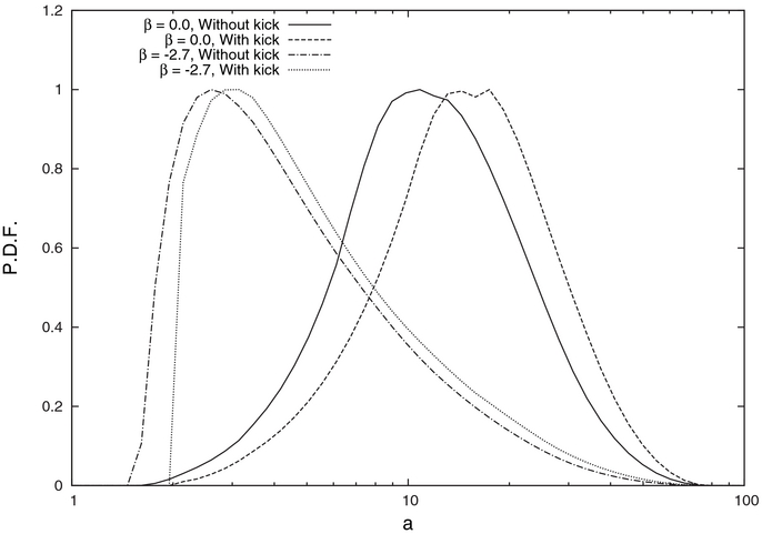
Zoom In Zoom Out Reset image size

Figure 11 shows the effect of varying β, i.e., the exponent of the q-distribution, on the a-distribution, which is quite strong. The steeply falling power law with β = −2.7 shifts the distribution's peak to much smaller values of a compared to the situation for the flat (β = 0) q-distribution. Again, here we find close similarities to previous results in the literature, i.e., Pfahl et al. (2003) for the β = 0 case, and Kalogera & Webbink (1998) for the β = −2.7 case, and again the former similarity is particularly striking. We emphasize that the general rise-and-fall shape of the a-distribution for pre-LMXBs seems both quite generic and confirmed by all previous calculations known to us, and that this shape stands in contrast to the generically flat or nearly flat shape at intermediate a's that we found for pre-HMXBs and HMXBs in Paper I.

Zoom In Zoom Out Reset image size